
"Stereoscopic technology certainly holds interesting possibilities once we get over the 'we must put the sword in the viewer's face' phenomenon."
After Effects and Nuke contain toolsets that may be considered "advanced." This does not mean that they are necessarily difficult to apply. However, they do tend to be unintuitive—or they are at least based on unusual algorithms or workflows. The tools include those that process HDRI, prepare multiple views for stereoscopic 3D, time-warp footage, retexture CG in the composite, simulate physical effects, and provide various scripting languages for customization or automation. There are no tutorials in this chapter. However, at the end, the reader is encouraged to use all the techniques discussed in this book to combine provided footage and image files creatively.

High Dynamic Range Imaging (HDRI) techniques store extremely large dynamic ranges. A dynamic range is the ratio of minimum to maximum luminous intensity values that are present at a particular location. For example, a brightly-lit window in an otherwise dark room may produce a dynamic range of 50,000:1, where the luminous intensity of the light traveling through the window is 50,000 times more intense than the light reflected from an unlit corner. Such a large dynamic range cannot be accurately represented with a low bit-depth. Even if you use a suitably large bit-depth, such as 16-bit with 65,536 tonal steps, the intensity values must be rounded off and stored as integers; this leads to inaccuracy. Hence, high dynamic range (HDR) image formats employ 16- or 32-bit floating-point architecture. The floating-point architecture supports a virtually unlimited number of tonal steps, plus it maintains the ability to store fractional values. (For more information on floating-points, see Chapter 2, "Choosing a Color Space.")
HDRI is commonly employed in professional photography. A common approach to taking HDR photographs follows these steps:
A camera is fixed to a tripod. Multiple exposures are taken so that every area of the subject is properly exposed (see Figure 12.1). Each exposure is stored as a standard 8-, 10-, 12-, or 16-bit low dynamic range (LDR) image.
The multiple exposures are brought into an HDR program, such as HDRShop or Photomatix, where they are combined into a single HDR image. The image is exported as a 16- or 32-bit OpenEXR,
.hdr, or a floating-point TIFF. Note that HDR refers to high dynamic range images in general, while.hdrrefers specifically to the Radiance file format. HDR image formats are discussed in the section "HDR Formats and Projections" later in this chapter.If the HDR image is destined for print, a limited tonal range is isolated by applying an exposure control, or the entire tonal range is compressed through tone mapping (which is described later in this chapter).

Figure 12.1. (Left) Three exposures used to create an HDR image (Right) Detail of tone-mapped result (HDR image by Creative Market)
HDR photography is often employed in the visual effects industry to capture the lighting on location or on set. The resulting HDR images are used by animators to light CG within a 3D program. Similar lighting approaches are occasionally applied by compositors in a compositing program. There are several approaches to these techniques:
A single HDR image captures an entire location or set. The image is loaded into an image-based lighting tool. The image is projected from the surface of a projection sphere toward a CG element at its center. A renderer utilizing radiosity, global illumination, or final gather is employed. The pixel values of the projected HDR image are thereby interpreted as bounced, ambient, or indirect light. In addition, the HDR information is used as a reflection source. (Although this process usually happens in a 3D program, some compositing packages are able to light 3D geometry with an HDR image; for a demonstration in Nuke, see the section "Environment Light and SphericalTransform" later in this chapter.)
HDR images of real-world light sources are mapped to planar projections or area lights, which are placed an appropriate distance from the CG camera and CG elements. A renderer utilizing radiosity, global illumination, or final gather converts pixel values into light intensity values. Such virtual lights are known as HDR lights.
HDR images of the set are projected onto a polygonal reproduction of the set. The point of view of the hero element (such as a CG character or prop) is captured and a new environmental HDR map is created. The new map is then used to light the hero element through an image-based lighting system. If the hero element moves through the shot, the environmental HDR map changes over time to reflect the changing point of view. Animated maps using this technique are referred to as animated HDRs. (For a simple demonstration of this process in Nuke, see the section "Creating Animated HDRs" later in this chapter.)
An HDR image is loaded into a compositing program. A light icon is interactively positioned in a viewer. Wherever the light icon rests, a higher exposure level within the HDR is retrieved. Thus, the compositor is able to light within the composite interactively while using the real-world intensity values contained within the HDR image.
Nuke supports the ability to light geometry with an HDR image through the Environment node. In addition, Nuke can convert between different styles of HDR projections with the SphericalTransform node. These nodes are described in the section "HDRI Support in Nuke" later in this chapter. Both After Effects and Nuke can read and manipulate various HDR file formats, which are described in the next section.
Here's a quick review of commonly used HDR formats. Additional information can be found in Chapter 2:
OpenEXR (
.exr) was created by Industrial Light & Magic. It is widely used in the visual effects industry. OpenEXR has a 16-bit half float and a 32-bit full float variation, both of which can support HDR photography.Radiance (
.hdr, .rgbe, .xyze) was developed by Greg Ward and was the first widely used HDR format.Floating-Point TIFF is a 16-bit half float or 32-bit full float variation of the common TIFF format. This format is the least efficient of the three and produces significantly larger file sizes.
When HDRI is employed for professional photography, the images are left in a recognizable form. That is, they remain rectangular with an appropriate width and height. When HDRI is used to light a scene within a 3D program or compositing program, however, the images must be remapped to fit a particular style of projection. Different projection styles are required by different image-based lighting tools, projections, and nodes. There are several different projection types:
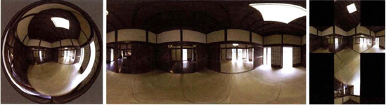
Light probe projections capture the reflection of an environment in a highly reflective chrome ball or sphere (see Figure 12.2). Through an HDR or paint program, the reflection of the camera or photographer is removed. This style has 180×180° and 360×360 variations. The 180×180° image is taken from a single point of view, while the 360×360 image is assembled from two views offset by 90°. Light probe images appear similar to those simply named mirrored ball. However, the light probe algorithm retains more information along the edge of the sphere when compared to the mirrored ball versions. Light probe HDRs are also referred to as angular.
Lat long projections are rectangular and often feature a complete panoramic view of a location (see Figure 12.2). This style of HDR is also referred to as spherical, latitude/longitude, and equirectangular.
Cubic cross projections feature an unfolded cube, which encompasses a complete 360° view of a location (see Figure 12.2). This style has vertical and horizontal variations.
The main disadvantage of HDR images is the inability to display their entire tonal range on a low-bit-depth monitor or television. There are two solutions to this predicament: choose a narrow tonal range through an exposure control or apply tone mapping. HDR-compatible programs provide exposure controls for the purpose of previewing or exporting at a lower bit depth. For example, Photoshop includes an Exposure slider through the 32-Bit Preview Options dialog box. After Effects provides the Exposure effect for the same purpose. Nuke's Grade node can be used to the same end.
Choosing a tonal range through an exposure control ignores or discards the remaining tonal range. In comparison, the process of tone mapping remaps the entire tonal range to a lower-bit-depth space, such as 8-bit. Hence, tone mapping creates an image where everything is equally exposed, leading to a low-contrast, washed-out look (see Figure 12.1 earlier in the chapter). The stylistic quality of tone mapping is prized by many photographers. However, tone mapping is generally not used in the realm of compositing unless such a stylistic look is desirable. Nevertheless, After Effects supports tone mapping through its HDR Compander effect. After Effects's and Nuke's support of HDR is discussed in detail later in this chapter.
Stereoscopy is any technique that creates the illusion of depth through the capture of two slightly different views that replicate human binocular vision. Because left and right human eyes are separated by a distinct distance, each eye perceives a unique view. Objects at different distances from the viewer appear to have different horizontal positions in each view. For example, objects close to the viewer will have significantly different horizontal positions in each view, while objects far from the viewer will have almost identical horizontal positions. The difference between each view is known as binocular or horizontal disparity. The horizontal disparity is measurable as an angle between two lines of sight, where the angle is defined as parallax. The human mind uses the horizontal disparity as a depth cue. When this cue is combined with monocular cues such as size estimation, the world is successfully perceived as three-dimensional. The process of yielding a depth cue from horizontal disparity is known as stereopsis.
The earliest form of stereoscopy took the form of stereoscopic photographs developed in the mid-1800s. Stereoscopic photos feature slightly divergent views that are printed side by side. When the photos are viewed through a stereoscope (a handheld or table-mounted viewer with two prismatic lenses), the illusion of depth is achieved (see Figure 12.3).
The stereoscopic process was applied to motion pictures in the late 1890s. The peak of commercial stereoscopic filmmaking occurred in the early 1950s with dozens of feature films released. By this point, the term 3-D referred to stereoscopic filmmaking (although earlier cartoons used the phrase to advertise multiplaning). While pre-2000 3-D films generally relied on anaglyph methods to create the depth illusion, post-2000 films usually employ polarization. In both cases, the audience member must wear a pair of glasses with unique lenses.

Anaglyphs carry left and right eye views; however, each view is printed with a chromatically opposite color. The views are overlapped into a single image (see Figure 12.4). Each lens of the viewer's glasses matches one of the two colors. For example, the left view is printed in red and the right view is printed in cyan. The left lens of the viewer's glasses is therefore tinted cyan, allowing only the red left view to been seen by the left eye. The right lens of the viewer's glasses is tinted red, allowing only the cyan right view to been seen by the right eye. Because cyan is used, blue and green portions of RGB color space are included. That said, it's possible to create anaglyphs with black-and-white images. Nevertheless, early color motion picture anaglyphs relied on red-green or red-blue color combinations (see Figure 12.4).

Polarization relies on an unseen quality of light energy. Light consists of oscillating electrical fields, which are commonly represented by a waveform with a specific wavelength. When the light oscillation is oriented in a particular direction, it is said to be polarized. Linear polarization traps the waveform within a plane. Circular polarization causes the waveform to corkscrew. When light is reflected from a non-metallic surface, it's naturally polarized; that is, the light energy is emitted by the surface in a specific direction. Sky light, which is sunlight scattered through Earth's atmosphere, is naturally polarized. Polarized filters take advantage of this phenomenon and are able to block light with specific polarization. For example, polarized sunglasses block light that is horizontally polarized (roughly parallel to the ground), thus reducing the intensity of specular reflections (which forms glare). Professional photographic polarizers can be rotated to target different polarizations. Stereoscopic 3-D systems apply polarized filters to the projected left and right views as well as to each lens of the viewer's glasses. The polarization allows each view to be alternately hidden from sight.
When a stereoscopic project is presented, there are several different projection and display methods to choose from:
Dual Projectors One projector is tasked with the left view, while a second projector is tasked with the right view. Early stereoscopic motion pictures, which relied on this method, employed anaglyph color filters. Current IMAX systems use a polarized projector lenses.
Passive Polarization A single projector alternatively projects left and right views. The views are retrieved from interlaced video footage (where each view is assigned to an upper or lower field) and filtered through a linear or circular polarization filter. As the left view is projected, the polarization of the viewer's right lens blocks the left view from the right eye. As the right view is projected, the polarization of the viewer's left lens blocks the right view from the left eye. The term passive is used because the viewer's glasses are not synchronized with the projection, as is possible with an active shutter system (see the next description). The frame rate of a passive polarization system may be quite high. For example, the RealD system projects at 144 fps, where each view of a single frame is shown three times (24 fps×2 views ×3).
Active Shutter A single projector or display is used in combination with shutter glasses, which contain polarizing filters and liquid crystals that can switch between opacity and transparency with the application of voltage. The voltage application is cued by an infrared emitter driven by the projector or display. Active shutter systems have the advantage of working with consumer digital projectors, televisions, and PC monitors. Active shutter systems can use either interlaced frames or checkerboard wobulation, whereby the two views are broken into subframes and intertwined in a fine checkerboard pattern.
There are several methods used to capture footage for a stereoscopic project. A common approach utilizes two cameras. The cameras are either positioned in parallel (side by side) or are converged so that their lines of sight meet at a particular point on set. To make the stereoscopic effect successful, the lenses must be the same distance apart as human eyes-roughly 2.5 inches. The distance between eyes is known as interocular distance. The distance between lenses is referred to as interaxial separation. The correct distance may be achieved with beamsplitters, mirrors, or lenses positioned at the end of optical fiber cables (see Figure 12.5). If such a setup is not possible on set, the footage for each view is transformed in the composite to emulate an appropriate distance.

Figure 12.5. A 1930s Leitz stereoscopic beamsplitter fed left and right views to a single piece of film (Image © 2009 by Jupiterimages)
When stereoscopic footage is prepared, a convergence point must be selected. A convergence point is a depth location where the horizontal disparity between the left and right eye views is zero (that is, the disparity is 0° parallax). When the footage is projected, objects in front of this point appear to float in front of the screen (possessing negative parallax). Objects behind the point appear to rest behind the screen (possessing positive parallax). If the footage is shot with converged cameras, the convergence point may be selected by the cinematographer while on the set. More often, however, it is more efficient to select a convergence point while the compositor is working in the composite.
After Effects and Nuke provide stereoscopic effects and nodes specifically designed for reading and preparing stereoscopic 3-D footage. These are discussed later in this chapter.
Time warping is a generic term for the retiming of footage. If the motion within a piece of film of video footage is too slow or too fast, the frame rate can be altered. Before the advent of digital filmmaking, this was achieved by skip printing or stretch printing motion picture film; with these techniques, film frames from the camera negative were skipped or repeated as positive film stock was exposed. Skipping or repeating frames is a basic time warping technique that continues to be applied by compositing programs. However, compositing programs have the advantage of frame blending, whereby sets of neighboring frames are averaged so that new, in-between frames are generated.
There are multiple approaches to frame blending. Simple frame blending merely overlaps neighboring frames with partial opacity. Advanced frame blending utilizes optical flow. Optical flow is a pattern created by the relative motion of objects as seen by an observer. In compositing, optical flow is represented by a 2D velocity field that places pixel motion vectors over the view plane (see Figure 12.6). Optical flow, as it's used for time warping, employs motion estimation techniques whereby pixels are tracked across multiple frames. By accurately determining the path a pixel takes, it is easier to synthesize a new frame. If a pixel starts at position A and ends at position B, it can be assumed that a point between A and B is suitable for a new, in-between position. (When discussing optical flow, pixels are point samples with a specific color value that can be located across multiple frames.) However, if the footage is high resolution, tracking every image pixel may prove impractical. Thus, optimization techniques allow the images to be simplified into coarser blocks or identified homogeneous shapes.

Figure 12.6. Detail of a 2D velocity field. In this example, the source footage is curling white smoke over a dark background.
Optical flow techniques have inherent limitations. For example, footage that contains inconsistent brightness, excessive grain or noise, or multiple objects moving in multiple directions is problematic.
After Effects and Nuke support a wide range of advanced techniques that include HDRI, time warping, stereoscopic preparation, and scripting. In addition, After Effects provides the ability to create dynamic, physically based simulations while Nuke allows you to remap UV texture space of pre-rendered CG.
After Effects offers several effects with which you can interpret HDR images, change the duration of a piece of footage, create stereoscopic images, automate functions with a script, and create particle simulations.
After Effects supports a 32-bit floating-point color space. As discussed in Chapter 2, you can set the Depth menu of the Project Settings dialog box to 32 Bits Per Channel (Float). In addition, the program can import OpenEXR, floating-point TIFF, and Radiance files (which include files with .hdr, .rgbe, and .xyze filename extensions). The program can write out the same floating-point formats. When an HDR image is written, the full 32-bit floating-point color space is encoded, even if the dynamic range is not fully visible through the viewer.
Because the tonal range of an HDR image file is far greater than the tonal range of an 8-bit or 10-bit monitor, it may be necessary to compress the range or select a specific exposure. The HDR Compander, the HDR Highlight Compression, and the Exposure effects are designed for these tasks.

Figure 12.7. (Top Left) An HDR image is brought into a 32-bit project. Due to the limited tonal range of the 8-bit monitor, it appears overexposed. (Top Right) The same image after the application of the HDR Compander effect with its Gain slider set to 10. (Bottom Left) The HDR Compander effect is placed before a Luma Key effect in order to compress the 32-bit space to a 16-bit tonal range. Normally, the Luma Key cannot operate in 32-bit space, as is indicated by the yellow warning triangle. (Bottom Right) The result of the Luma Key, which is able to operate with the addition of the HDR Compander effect. A sample After Effects project is included as compander.aep in the Tutorials folder on the DVD.
The HDR Compander effect (in the Effect → Utility menu) is specifically designed to compress a 32-bit tonal range down to 8-bit or 16-bit color space, where lower-bit-depth effects can be applied; once those effects are applied, a second iteration of the HDR Compander effect can expand the tonal range back to 32 bits.
As an example, in Figure 12.7, a floating-point TIFF of a shelf is imported into a project with its Depth menu set to 32 Bits Per Channel (Float). A sample pixel within its brightness area has a value of 3460, 1992, 0 on an 8-bit scale of 0 to 255. The same pixel has a value of 444, 662, 255, 918, 0 when examined using a 16-bit scale of 0 to 32,768. The same pixel has a value of 13.57, 7.81, 0 when examined using a 0 to 1.0 scale. In this situation, the brightest pixel is 13.57 times brighter than the 255, 32,768, or 1.0 limit. (You can change the scale the Info panel uses to display pixel values by changing the Info panel menu to 8-bpc, 10-bpc, 16-bpc, or Decimal.) Hence, the TIFF possesses values far beyond range that an 8-bit monitor can display. In addition, the TIFF possesses values beyond the range in which an 8- or 16-bit effect can operate.
When the HDR Compander effect is applied to the TIFF layer, the effect's Mode menu is set to Compress Range and the Gain slider is set to 10. When the Info panel menu is set to Decimal (0.0-1.0), the same pixel values become 1.36, 0.78, 0. The Gain slider operates with the following formula: input pixel value / Gain. The formula holds true whether the Info panel menu is set to 8-bpc, 10-bpc, or 16-bpc. The Gain slider operates in a linear fashion. That is, all areas of the tonal range are compressed equally. You can bias a particular area of the tonal range, however, by adjusting the effect's Gamma slider, which applies a gamma curve to the result. For example, Gamma values above 1.0 will favor the low end of the tonal range while values below 1.0 will favor the high end of the tonal range.
If a second iteration of the HDR Compander is added with the Mode menu set to Expand Range and the Gain slider set to match the first HDR Compander iteration, the original tonal range is restored. Note that the second HDR Compander effect is optional and is useful only if you plan to render out 32-bit floating-point image sequences.
Although you can apply the Exposure effect to 8- or 16-bit images, as discussed in Chapter 4, its Exposure slider is designed for 32-bit footage. For example, in Figure 12.8, a light probe .hdr of a brightly colored room appears underexposed when first imported. If Exposure is set to 3, the room becomes easier to see, but the reflected windows remain overexposed. If Exposure is set to −2, the windows are properly exposed, but the rest of the room becomes darker. The Exposure effect multiplies each pixel value by a constant and is not concerned with the overall tonal range. The unit of measure of the Exposure slider is an f-stop; each whole f-stop value has twice the intensity of the f-stop below it. By default, the effect is applied equally to all channels. However, you can set the Channels menu to Individual Channels and thus produce separate red, green, and blue controls. Note that the effect operates in linear (non-gamma-adjusted) color space and not the inherent color space of the imported footage. However, you can override this trait by selecting the Bypass Linear Light Conversion check box.
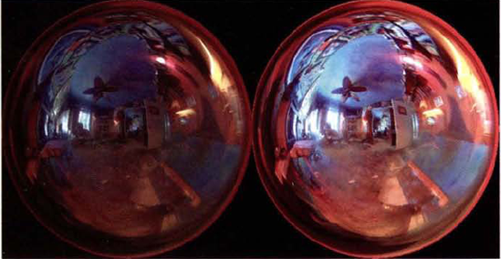
Figure 12.8. (Left) A light probe image appears underexposed when imported into a 32-bit project. (Right) The same light probe gains better balance when an Exposure effect is applied with its Exposure slider set to 3. A sample After Effects project is included as exposure.aep in the Tutorials folder in the DVD.
To combat highlights within HDR images that become overexposed, After Effects provides the HDR Highlight Compression effect (in the Effect → Utility menu). For example, if the Exposure effect is applied to the floating-point TIFF of the shelf with an Exposure slider set to −5.5, the wall below the shelf light remains overexposed with RGB values over 1,000 on an 8-bit scale (see Figure 12.9). If the HDR Highlight Compression effect is applied, the overexposed area is tone mapped so that the values no longer exceed the 8-bit monitor color space. The HDR Highlight Compression effect has a single slider, Amount, which controls the strength of the tone mapping.

The 3D Glasses effect (in the Effect → Perspective menu) creates stereoscopic images. To use the effect, follow these steps:
Create a new composition. Import the left eye view and right eye view footage. LMB+drag the footage into the outline layer. Toggle off the Video switches for each new layer.
Create a new Solid (Layer → New → Solid). With the Solid layer selected, choose Effect → Perspective → 3D Glasses. In the Effect Controls panel, change the 3D Glasses effect's Left View menu and Right View menu to the appropriate view layer names.
Change the 3D View menu to the anaglyph style of choice. For example, switching the menu to Balanced Colored Red Blue tints the left view cyan and the right view red (see Figure 12.10).

Figure 12.10. (Top Left) Left view (Bottom Left) Right view (Top Right) 3D Glasses effect properties (Bottom Right) Resulting red-cyan anaglyph. A sample After Effects project is included as stereoscopic.aep in the Tutorials folder on the DVD.
The 3D View menu has additional settings, which are tailored toward specific outputs:
Stereo Pair sets the left and right view side by side. You can use this mode to create a cross-eyed stereo view. Cross-eyed stereo does not use glasses but requires the viewer to cross their eyes slightly until a third stereo image appears in the center. However, for a cross-eyed view to be successful, the left and right images must be swapped; you can perform the swap with the 3D Glasses effect by toggling on the Swap Left-Right property.
Interlace Upper L Lower R places the left view into the upper field and the right view into the lower field of an interlaced output. This mode is necessary when preparing stereoscopic footage for a polarized or active shutter system. If toggled on, the Swap Left-Right property switches the fields.
Red Green LR and Red Blue LR create red-green and red-blue color combinations based on the luminance values of the left and right view layers.
Balanced Colored Red Blue creates a red-blue color combination based on the RGB values of the left and right view layers. This allows the resulting anaglyph to retain the layers' original colors. However, this setting may produce ghosting, which occurs when the intensity of one stereo color exceeds that of the paired color. For example, the red view may bleed into the cyan view. You can adjust the Balance slider to reduce ghosting artifacts; in essence, the slider controls the amount of saturation present for the paired stereo colors.
Balanced Red Green LR and Balanced Red Blue LR produce results similar to Red Green LR and Red Blue LR. However, the settings balance the colors to help avoid ghosting artifacts.
You can adjust the horizontal disparity and the location of the convergence point by raising or lowering the Convergence Offset value. Positive values slide the right view to the right and the left view to the left. This causes the convergence point to occur closer to the camera and forces a greater number of objects to appear behind the screen. Negative Convergence Offset values have the opposite effect. You can identify a convergence point in an anaglyph by locating the object that does not have overlapping colors. For example, in Figure 12.10, the convergence point rests at the central foreground tree.
After Effects includes several approaches to time warping imported footage. These include time stretching, blending, and remapping.
The simplest way to time-warp a piece of footage is to apply the Time Stretch tool (Layer → Time → Time Stretch). In the Time Stretch dialog box, the Stretch Factor value determines the final length of the footage. For example, entering 50% makes the footage half its prior length, while 200% makes the footage twice its prior length. The Time Stretch tool does not blend the frames, however. If the footage is lengthened, each frame is duplicated. If the footage is shortened, frames are removed. This may lead to judder in any motion found in the footage.

Figure 12.11. (Top Left) Detail of time-stretched footage with Frame Mix blending. Significantly lengthening the duration of the footage (in this case, 200%) creates overlapping images of the ship. (Top Right) Same time-stretched footage with Pixel Motion blending. (Bottom) Frame Blending switches in the layer outline. A sample After Effects project is included as frame_blending.aep in the Tutorials folder on the DVD.
To avoid judder, you can apply one of two frame-blending tools, both of which are found under Layer → Frame Blending. Frame Mix applies an efficient algorithm that is suitable for previews and footage that contains fairly simple motion. Pixel Motion applies a more advanced algorithm that is more appropriate for footage that has been significantly stretched (whereby the motion has been slowed down). Once frame blending has been applied, you can switch between Frame Mix and Pixel Motion styles by toggling the Frame Blending layer switch (see Figure 2.11). The backslash, which is considered draft quality, activates Frame Mix, while the forward slash, considered high quality, activates Pixel Motion. Frame blending, with either tool, averages the pixels between two original frames, thus creating new in-between frames. Frame-blended frames, in general, are softer than the original frames. (To see frame blending in the viewer, you must toggle on the Frame Blending composition switch.)
A limitation of the Time Stretch tool is its linear nature. If you wish to change the duration of a piece of footage in a nonlinear fashion, use the Time Remapping tool. To use the tool, follow these steps:
Select the layer you wish to remap. Choose Layer → Time → Enable Time Remapping. A Time Remap property is added to the layer in the layer outline (see Figure 12.12).
Toggle on the Include This Property In The Graph Editor Set button beside the Time Remap property name. Open the Graph Editor by toggling on the Graph Editor composition switch at the top right of the layer outline.
By default, the Time Remap curve runs from 0 to 1.0 over the current duration of the footage. Manipulate the Time Remap curve shape to change the speed of the motion contained within the footage. For example, to give the motion a slow start, a fast middle, and a slow end, create an S-shaped curve in the value graph view (see Figure 12.13). You can use any of the standard Graph Editor tools and options to change the curve shape. (See Chapter 5 for more information on the Graph Editor.)
If you wish to shorten or lengthen the footage, select the top-right curve point and LMB+drag it to a new frame number. If you lengthen the footage, you will also need to extend the footage bar in the timeline view of the Timeline panel.
To frame-blend the result, activate Frame Mix or Pixel Motion (see the prior section). If the Time Remap curve is significantly altered, it will be necessary to use Pixel Motion to produce acceptable results. To remove a Time Remap property from a layer, toggle off the Stopwatch button beside the Time Remap name.
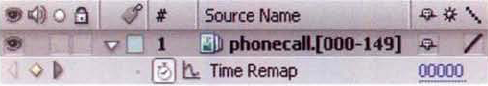

Figure 12.13. (Top) Default Time Remap curve in the value view (Bottom) Curve reshaped to create a slow start and end for the motion contained within the footage. A sample After Effects project is included as time_remap.aep in the Tutorials folder on the DVD.
The Timewarp effect (Effect → Time → Timewarp) operates in a manner similar to the Time Stretch tool. However, if the Speed property is set to a value below 100%, the footage is lengthened. If the Speed property is set to a value above 100%, the footage is shortened. In either case, the footage bar in the Timeline panel remains the same length. If the footage is shortened, the last frame of the footage is held until the end of the footage bar. If the footage is lengthened, any frame beyond the end of the footage bar is ignored. You can activate Frame Mix or Pixel Motion frame blending through the Method menu. Timewarp differentiates itself by providing a Tuning section if the Method menu is set to Pixel Motion. The Tuning section includes the following important properties:
Vector Detail determines how many motion vectors are drawn between corresponding pixels of concurrent original frames. The vectors are necessary for determining pixel position for blended frames. A value of 100 creates one motion vector per image pixel. Higher values produce more accurate results but significantly slow the render.
Filtering selects the convolution filter used to average pixels. If this property is set to Normal, the filtering is fairly fast but will make the blended frames soft. If it's set to Extreme, the blended frames will regain their sharpness but the render time is impacted greatly.
In addition, the effect provides motion blur for blended frames if the Enable Motion Blur check box is selected (see Figure 12.14). You can adjust the blur length by setting the Shutter Control menu to Manual and changing the Shutter Angle value. The length of the motion blur trail, which is driven by the virtual exposure time, is based on the following formula: exposure time = 1 / (360 / Shutter Angle) × frames per second). The larger the shutter angle, the longer the motion blur trail becomes.

Several additional time tools and effects are included in the Layer → Time and the Effect → Time menus. Descriptions of the most useful effects follow:
Time-Reverse Layer This tool reverses the frame order of a layer. What runs forward is made to run backward.
Freeze Frame This tool adds a Time Remap property and sets a keyframe at the current frame. The keyframe's interpolation is set to Hold, which repeats the frame for the duration of the timeline. However, you can alter the curve in the value view of the Graph Editor to make the Freeze Frame effect occur at a certain point in the timeline. For example, in Figure 12.15, frames 1 to 4 progress normally, while frame 5 is "frozen" for the remainder of timeline. In this situation, a keyframe must be inserted into the curve at frame 1, and both keyframe tangent types must be changed from Hold to Linear.
Echo The Echo effect purposely overlaps frames for a stylized result. The Echo Time (Seconds) property sets the time distance between frames used for the overlap. The Number Of Echoes slider sets the number of frames that are blended together. For example, if the project is set to 30 fps, Echo Time is set to 0.066, Number Of Echoes is set to 2, and the timeline is currently on frame 1, then frame 1 is blended with frames 3 and 5. The value 0.033 is equivalent to 1 frame when operating at 30 fps (1 / 30). By default, the effect adds the frames together, which often leads to overexposure. To defeat this, you can adjust the Starting Intensity slider or choose a different blending mode through the Echo Operator menu.
Posterize Time The Posterize Time effect locks a layer to a specific frame rate regardless of the composition settings. This allows you to create a step frame effect where each frame is clearly seen as it is repeated. The Frame Rate property sets the locked frames per second.
Time Difference The Time Difference effect determines the color difference between two layers over time. Each output pixel value is based on the following formula: ((source pixel value - target pixel value) × Contrast property percentage) + 128. The source layer is the layer to which the effect is assigned. The target layer is determined by the effect's Target menu. If the source and target pixel are identical, the output pixel value is 128. The Time Difference effect is useful for generating a moving matte. For example, in Figure 12.16, an empty greenscreen plate serves as the target layer, while footage of a model serves as the source layer. The background is removed from the output.
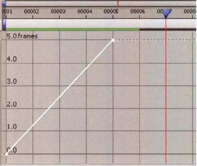
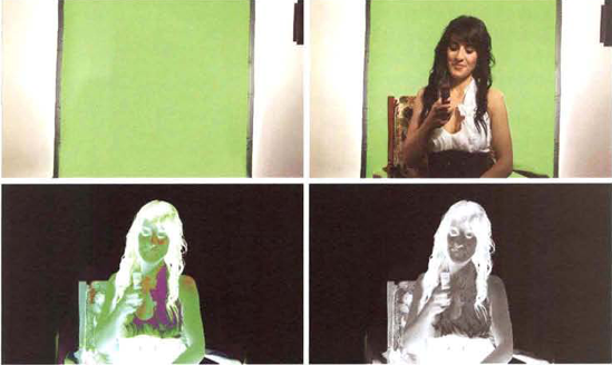
Figure 12.16. (Top Left) Empty background plate (Top Right) Plate with model (Bottom Left) Result of Time Difference effect with Absolute Difference toggled on and Alpha Channel menu set to Original (Bottom Right) Result seen in alpha channel with Absolute Difference toggled on and Alpha Channel menu set to Lightness Of Result. A sample project is included as time_difference.aep in the Tutorials folder on the DVD.
If the Absolute Difference property is toggled on, the formula switches to the following: (absolute value of (source pixel value - target pixel value))×(Contrast property percentage×2). By default, the alpha for the output is copied from the source layer. However, you can alter this behavior by switching the Alpha Channel menu to options that include, among others, the target layer, a blended result of both layers, and a grayscale copy of the output (Lightness Of Result).
After Effects includes a number of effects designed for simulation, whereby a phenomenon is re-created as the timeline progresses. The simulations either replicate basic laws of physics or re-create the proper look of a phenomenon in the real world. The simulations include generic particles, raindrops, soap bubbles, snow, and foam. Since the list of effects and their properties is quite long, only the Particle Playground effect is covered in this section. Additional documentation on non-third-party effects, such as Card Dance, Caustics, and Shatter, are included in the Adobe help files.

Figure 12.17. (Top) Default particle emission with the emitter at the base of the particles (Bottom) Default Particle Playground properties
The Particle Playground is one of the most complex effects in the program. The generated particles are able to react to virtual gravity and interact with virtual barriers. To apply the effect, you can follow these steps:
Create a new Solid layer. With the layer selected in the layer outline of the Timeline panel, choose Effect → Simulation → Particle Playground.
By default, dot particles are generated from a "cannon." That is, they are shot upward from an emitter. The emitter is represented in the viewer by a red circle (see Figure 12.17). You can reposition the emitter interactively by LMB+dragging it. To see the particle simulation, play back the timeline from frame 1.
By default, the particles possess a slow initial velocity. Within a short time, they begin to fall toward the bottom of the frame through a virtual gravity. To adjust the strength of the gravity, change the Force property (in the Gravity section). You can alter the direction of the gravity, and thus emulate wind, by changing the Direction property. To alter the number of particles, initial velocity, initial direction, and randomness of movement, adjust the properties in the Cannon section (see Figure 12.17). To widen the throat of the virtual cannon, raise the Barrel Radius property. To change the size of the particles, adjust the Particle Radius property. Since the particles are dots, they will remain square.
If you wish to generate particles from a grid instead of the cannon, set Particles Per Second in the Cannon section to 0 and raise the values for the Particles Down and Particles Across properties in the Grid section. With the grid emitter, particles are born at each grid line intersection. The size of the grid is set by the Width and Height properties, although the grid resolution is determined by Particles Down and Particles Across. If Particles Down and Particles Across are both set to 2, the grid has a resolution of 2×2, even if it's 100×100 pixels wide.
The red, square particles are rarely useful as is. You can take two approaches to making them more worthy of a composite—apply additional effects or use the Layer Map property. Two examples follow.
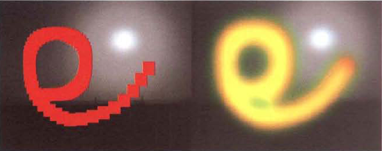
To create a light trail with the Particle Playground effect (where a moving light streaks over a long exposure), choose the grid style of particle generation. Set the Particles Across and Particles Down properties to 1.0. So long as the Force Random Spread property (in the Gravity section) is set to 0, the particles will flow in a perfectly straight line. To prevent the particles from drifting, set the Force property to 0. To create the illusion that the light is streaking, animate the Position property (in the Grid section) moving over time. You can then blur and color adjust the result before blending it over another layer (see Figure 12.18).
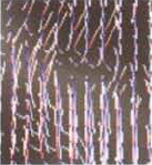
To use the Particle Playground's Layer Map property, prepare a bitmap sequence that is suitable for mapping onto a particle. For instance, create a low-resolution sequence featuring a bird, bat, or insect flapping its wings (see Figure 12.19). Import the bitmap sequence into a project. LMB+drag the sequence from the Project panel to the layer outline of the composition that carries the Particle Playground effect. Toggle off the Video switch beside the sequence layer to hide it. Change the Particle Playground's Use Layer menu (in the Layer Map section) to the sequence layer name. The sequence is automatically mapped onto the particles. If the bitmaps include alpha, the transparency is applied to the particles. To loop a short sequence, increase the Loop value (found in the Interpret Footage dialog box). To offset each particle so that all the particles aren't lock-stepped in their animation, incrementally raise the Random Time Max value (which is based on seconds). For example, in Figure 12.19, the bitmap sequence has only eight frames, so Random Time Max is set to 0.1. To randomize the motions of the particles, adjust the Direction Random Spread, Velocity Random Spread, and Force Random Spread properties. To add motion blur to the particles, toggle on the Motion Blur layer switch; to see the blur in the viewer, toggle on the Motion Blur composition switch.

Two scripting methods are supported by After Effects: ExtendScript and expressions. ExtendScript is a programming language that allows you to write external scripts to control the program. Expressions provide a means to link and automate various properties.
After Effects supports scripting through the Adobe ExtendScript language. ExtendScript is an extended variation of JavaScript. ExtendScript is suitable for performing complex calculations beyond the capacity of standard effects, automating repetitive tasks, undertaking "search and replace" functions, communicating with outside programs, and creating custom GUI dialog boxes.
Each time After Effects launches, it searches the Scripts folder (for example, C:Program FilesAdobeAdobe After Effects CS3Support FilesScripts). Encountered scripts are accessible through the File → Scripts menu. You can also manually browse for a script file by choosing File → Scripts → Run Script File.
ExtendScript files carry the .jsx filename extension and are text based. You can edit a script in a text editor or through the built-in After Effects JavaScript editor, which you can launch by choosing File → Scripts → Open Script Editor. The Script Editor offers the advantage of automatic debugging and color-coded syntax.
Each ExtendScript script must begin with an opening curly bracket { and end with a closing curly bracket }. Lines that are not part of conditional statements or comments end with a semicolon. Comment lines, which are added for notation, begin with a double slash //. An ExtendScript script may be several pages long or as short as this example:
{
    //This script creates a dialog box
    alert("Compositing Rules!");
}
ExtendScript is an object-oriented programming language and therefore includes a wide array of objects. Objects, many of which are unique to After Effects, are collections of properties that perform specific tasks. Optionally, objects carry methods, which allow the object to operate in a different manner based on the specific method. The syntax follows object.method(value). Here are a few example objects, which are demonstrated by the demo.jsx script in the Tutorials folder on the DVD:
alert("message"); writes a message in pop-up dialog box.app.newProject();creates a new project after prompting you to save the old project.app.project.save();saves the current project so long as it has been saved previously.scriptFile.open();, scriptFile.read();, andscriptFile.close();open, read, and close a separate JSX script file, respectively.
Although many objects in ExtendScript are "ready-made," it's possible to create new objects within a script. The creation of an object is tasked to a constructor function, which defines the properties of the object. For example, in the demo.jsx script, var my_palette = new Window("palette","Script Demo"); creates a new object based on the constructor function named Window. The resulting my_palette object creates the dialog box GUI.
ExtendScript supports the use of variables through the var function. There are three common variables types:
var test = 100;         integer
var test = 12.23;       float
var test = "Finished";  string
Once a variable is declared, it's not necessary to use var when updating the variable value. ExtendScript supports common math operators. These include + (add), - (subtract), *(multiply), and / (divide).
Expressions, which are programmatic commands, link two or more properties together. A destination property is thereby "driven" by one or more source properties, whereby the destination receives the source values.
After Effects expressions rely on two naming conventions:
section.property[channel] effect("name")("property")
section refers to the section in the layer outline where the property resides. For example, Transform is a section while Opacity is a property. When a property has more than one component that can be animated, it earns a channel. For example, X, Y, Z and Red, Green, Blue are channels. Channels are represented by a position number starting with 0. Hence, X, Y, Z channels are given the positions 0, 1, 2. When an effect property is used, it's signified by the effect prefix. The effect name, such as Fast Blur, is contained in the first set of quotes.
To create an expression, follow these steps:
Select the property name in the layer outline and choose Animation → Add Expression. An expandable Expression field is added to the timeline to the right of the property name (see Figure 12.20). The name of the property and its channel is added to the Expression field.
To finish the expression, click the Expression field to activate it for editing. Type the remainder of the expression. If the expression is successful, the Enable Expression button is automatically toggled on and the property values turn red. If the expression fails due to mistyping, syntax error, or mismatched channels, the Enable Expression button remains toggled off and a yellow warning triangle appears beside it. In addition, a pop-up warning box identifies the error.

You can also pull property and channel names into the field by using the Expression Pick Whip tool. To use this tool, LMB+click and hold the Expression Pick Whip button. Without letting go of the button, drag the mouse to another property or channel (on any layer). A line is extended from the button to the mouse. Valid properties and channels turn cyan. Release the mouse over a property or channel. The property name and channel(s) are added to the Expression field. To prevent the Expression Pick Whip tool from overwriting the current property, add an = sign before using it. For example, if you create a new expression and the expression reads transform.position, update the expression to read transform.position= before using the Expression Pick Whip tool.
A simple expression equates one property to another. For example, you can enter the following:
transform.position=thisComp.layer("Solid1").transfrom.positionWith this expression, the Solid1 layer provides Position property values that drive the position of the layer with the expression. You can make expressions more complex by adding math operators. Basic operators include + (add), - (subtract), * (multiply), / (divide), and × −1 (invert). To double a value of a source property, include ×2 in the expression. To reduce the value by 25%, include /4 in the expression. An expression can contain more than one source property and/or channel. For example, you can enter the following expression:
transform.opacity=
transform.position[1]-effect("Brightness & Contrast")("Brightness")
With this expression, the Opacity value is the result of the layer's Position Y value minus the Brightness value of a Brightness & Contrast effect.
To delete an expression, select the property name in the later outline and select Animation → Remove Expression. You can temporarily turn off an expression by toggling off the Enable Expression switch (see Figure 12.20 earlier in this section). To insert expression functions into the Expression field, click the Expression Language Menu button and choose a function from the menu. Functions are code words that launch specific routines or retrieve specific values.
With Nuke, you can light a scene with an HDR image, prepare anaglyph stereoscopic footage, apply optical flow, automate functions with scripts and expressions, and retexture CG renders.
Nuke operates in 32-bit floating-point linear color space at all times. Lower bit-depth footage is converted to 32-bit as it's imported. The composite is viewed at a lower bit depth through the viewer, which applies a LUT determined by the project settings.
Nuke reads and writes .hdr, OpenEXR, and floating-point TIFF formats. To examine or utilize different exposure ranges within an HDR image, you can apply a Grade node and adjust the Whitepoint slider.
In addition, Nuke supplies the SoftClip node (in the Color menu), which compresses an HDR image's tonal range to a normalized range of 0 to 1.0. The node's Conversion menu determines whether the image's brightness or saturation is preserved. The Softclip Min and Softclip Max sliders determine the value range within the HDR that's compressed.
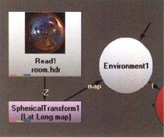
The Environment light allows you to create reflections and specular highlights in a 3D environment with an HDR bitmap. Assuming you have a 3D scene set up with geometry (see Chapter 11 for more detail), you can follow these steps:
Import an HDR bitmap through a Read node. A sample OpenEXR file is included as
room.exrin the Footage folder of the DVD. With the Read node selected, RMB+click and choose Transform → SphericalTransform. With the SphericalTransform node selected, RMB+click and choose 3D → Lights → Environment. Connect the Environment1 node to the appropriate Scene node (see Figure 12.21).Open the SphericalTransform node's properties panel. This node is designed to convert an environment bitmap, such as an HDR file, from one projection style to another. Change the Output Type menu to Lat Long Map. Lat long maps are designed to fit spherical projections (in fact, they are often referred to as spherical maps). Change the Input Type menu to the appropriate projection style. For a review of projection types, see the section "HDR Formats and Projections" earlier in this chapter. In the case of
room.exr, the menu should be changed to Angular Map 360.For the Environment light to have an effect on geometry, the geometry must be connected to a shader that possesses specular quality. The strength of the light's influence is therefore controllable through the shader's Specular, Min Shininess, and Max Shininess parameters.
You can adjust the overall brightness of the Environment light through the Environment node's Intensity slider. If Intensity is high and there are no other lights in the scene, the Environment light creates a strong reflection on the surface (see Figure 12.22). If other lights are present, the Environment light's influence is diminished; however, the light colors will be visible in the areas where there is a strong specular highlight. The Environment light's influence is also affected by the shader's Diffuse parameter. If Diffuse is set to 0, the surface will appear mirror-like. If the resulting reflection appears too sharp, you can blur it by raising the Environment node's Blur Size value. If the Diffuse value is high and other lights are present in the scene, the Environment's light contribution is reduced (see Figure 12.22).
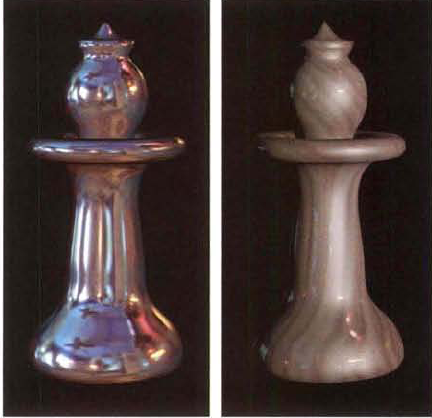
Figure 12.22. (Left) Reflection on 3D chess piece created by Environment light node when no other lights are present (Right) More subtle reflection created when a Direct light node is added to the scene
The position and scale of the Environment light icon does not affect the end result. However, the rotation does. You can change the Rotate XYZ values of the Environment node or the RX, RY, and RZ values of the SphericalTransform node to offset the resulting reflection along a particular axis.
As mentioned earlier in this chapter, an animated HDR is a rendered sequence from the point of view of a CG character or prop that is used for lighting information. The creation of an animated HDR generally occurs in two steps: (1) a CG re-creation of an set is modeled and textured with HDR photos captured at the real location, and (2) the point of view of the character or prop is captured through an animated camera and is rendered as a spherically mapped floating-point image sequence. You can spherically map the view of a camera in Nuke by setting the Camera node's Projection menu (in the Projection tab of the properties panel) to Spherical.

Figure 12.23. (Top) First frame of animated HDR sequence created by rendering a Camera node with its Projection property set to Spherical (Bottom) Last frame of sequence
As an example of this process, in Figure 12.23, the 3D hallway created in Chapter 11 is reutilized. The point of view of the animated cube is converted to a spherically mapped image sequence. This requires that the Camera1 node follows the cube's motion path exactly. To do this, the Cube1 node's animation is exported as a Chan file. The Chan file is then imported into the Camera1 node. Since the translation is desired but the rotation is not, the resulting rotation keyframes are deleted. An extra card is placed at the hall opening to prevent a black hole from appearing; the card is textured with a copy of the door photo. To prevent the cube from appearing in the render, it's temporarily disconnected from the Scene1 node. The Camera1 node's Projection menu is set to Spherical and an OpenEXR image sequence is rendered. (Although the 3D hallway is textured with low-dynamic-range bitmaps and is lit with standard Nuke lights, the process is essentially identical to one using a set textured with HDR bitmaps and lit with HDR lights.) A sample Nuke file for this step is included as animated_hdr_a.nk in the Tutorials folder on the DVD.

Figure 12.24. (Top) Node network created to light the cube with a spherically mapped, animated HDR (Bottom) Three frames from the resulting render of the cube. Variations in light quality are due to the change in the cube's rotation relative to its point of view as captured by the OpenEXR sequence.
The resulting OpenEXR sequence can be used for lighting information if it's loaded into a Read file and the Read file is connected to an Environment light node. However, the Environment light is only able to use the image sequence for the specular lighting component. This is suitable for creating a reflection pass or roughly emulating the diffuse lighting quality. For example, in Figure 12.24, the OpenEXR is brought into an adapted script. The 3D hallway and light are removed. The cube remains. The Phong1 node, however, is connected to the Read2 node through the MapS (specular) connection. The Phong1 node's Diffuse property is set to 0, Specular is set to 4, Min Shininess is set to 2, and Max Shininess is set to 2. To prevent flickering and distinct reflective patterns from appearing across the cube, the Read1 node, which carries the OpenEXR sequence, is connected to a Blur node with its Size property set to 15. Although the Environment light does not move during the animation, the view of the cube updates with each frame of the OpenEXR. The lighting therefore changes based on the cube's rotation relative to its point of view as captured by the OpenEXR sequence. For example, any side of the cube pointing downward is rendered darker as the view in that direction sees the carpet, which is less intensely lit than the walls. A sample Nuke file for this step is included as animated_hdr_b.nk in the Tutorials folder on the DVD.
Nuke can create anaglyphs and interlaced stereoscopic outputs appropriate for polarized and active shutter systems. You can combine views, split views, and separate various parameters for individual views. In addition, the program takes advantage of the OpenEXR format and is able to store multiple views within a single file.
To set up a stereoscopic script, follow these steps:
Choose Edit → Project Settings. In the properties panel, switch to the Views tab. Click the Set Up Views For Stereo button. A left and right view are listed in the Views field. You can switch between the views by clicking the Left or Right button that's added to the Viewer pane (see Figure 12.25). You can color-code any future connection lines by selecting the Use Colors In UI check box in the properties panel. By default, left view outputs are color-coded red and right view outputs are color-coded green.
Create two Read nodes. Load the left view into one Read node and the right view into the second Read node. With no nodes selected, RMB+click and choose View → Join Views. Connect the left-view Read node to the Left input of the JoinView1 node. Connect the right-view Read node to the Right input of the JoinView1 node. Connect a viewer to the JoinView1 node. You can look at the left and right view in the viewer by clicking the Left and Right buttons.

To convert two views to a single anaglyph image, connect an Anaglyph node (in the Views → Stereo menu) to a JoinViews node. The Anaglyph node converts each view into a monochromatic image. The left view is filtered to remove blue and green. The right view is filtered to remove red. The output of the node contains a red left view superimposed over a cyan right view (see Figure 12.26). The output is thus ready for viewing with red-cyan anaglyph glasses. You can write out the combined view with a standard Write node.

Figure 12.26. (Left) Two views combined with a JoinViews node and converted with an Anaglyph node (Right) Resulting Anaglyph. A sample Nuke script is included as anaglyph.nk in the Tutorials folder on the DVD.
The saturation of the anaglyph is controlled by the Amtcolour slider. If Amtcolour is set to 0, the anaglyph becomes black and white. High Amtcolour sliders maximize the colors contained within the original images but may lead to ghosting. You can invert the colors, thus making the right view red, by selecting the Anaglyphs node's (Right=Red) check box. You can adjust the horizontal disparity and the location of the convergence point by raising or lowering the Horizontal Offset value. Positive values slide the left view to the left and the right view to the right. This causes the convergence point to occur closer to the camera, which places a greater number of objects behind the screen. Negative Horizontal Offset values cause the convergence point to occur farther from the camera, which places a greater number of objects in front of the screen.
You can also change the convergence point by using the ReConverge node (Views → Stereo → ReConverge). However, the ReConverge node requires that the left and right views are carried as two separate channels in an OpenEXR file. In addition, the node requires a disparity field channel. A disparity field maps pixels in one view to the location of corresponding pixels in the second view. A specialized plug-in, such as The Foundry's Ocula, is required in this case. Disparity fields are also necessary to transfer Paint node strokes from one view to another. The Ocula plug-in also provides support for interlaced and checkerboard stereoscopic output, which is otherwise missing from Nuke.
You can write left and right views into a single OpenEXR file. If stereo views have been set up through the Project Settings properties panel, a Write node automatically lists the left and right views through its Views menu (see Figure 12.27). Once the OpenEXR is written, it can be reimported through a Read node. If an OpenEXR contains multiple views, a small V symbol appears at the top left of the Read node icon. You can connect a viewer to the Read node and switch between left and right views by clicking the Left and Right buttons in the Viewer pane.
Figure 12.27. (Left) View menu in a Write node's properties panel (Right) V symbol at top left of Read node signifying multiple views
Additionally, you can force the left and right views to be written as separate files by adding the %V variable to the File cell of the Write node. For example, entering filename.%V.exr will add the view name to each render.
If you connect a node to a Read node that carries a multi-view OpenEXR, the connected node affects both views equally. However, if stereo views have been set up through the Project Settings properties panel, each node parameter receives a View menu button (to the immediate left of each Animation button). If you LMB+click a View menu button and choose Split Off Left or Split Off Right from the menu, the parameter is broken into left and right view components (see Figure 12.28). To access each component, click the small arrow to the immediate right of the parameter name.
If an OpenEXR contains both views, you can extract a single view by connecting a OneView node (in the Views menu). The OneView node carries a single parameter, View, with which you select Left or Right. The OneView node allows you to manipulate one view without disturbing the other.
If you need to flop the views so that the left becomes right and the right becomes left, connect a ShuffleViews node (in the Views menu). Once the ShuffleViews node is connected to an output with two views, click the Add button in the node's properties panel. A Get column and From column appear. The Get column determines what view is being affected. The From column determines what source is used for the selected view. To swap the left and right views, click the Add button twice and click the buttons to match Figure 12.29.


Finally, you can use a multi-view OpenEXR in the following ways:
You can connect an Anaglyph node directly to a Read node that carries an OpenEXR with two views.
To examine two views simultaneously in the viewer, connect a SideBySide node (in the Views → Stereo menu). The SideBySide node will create a cross-eyed stereo view if the left and right views are first swapped with a ShuffleViews node (that is, the left view should be on the right and the right view should be on the left).
To blend two views into a single view, connect a MixViews node (in the Views → Stereo menu). The blend is controlled by the Mix slider.
Nuke includes several nodes with which you can stretch, shorten, and blend footage.
The simplest way to time-warp a piece of footage is to connect a Retime node (Time → Retime). In the Retime node's properties panel, Speed determines the final length of the footage. For example, entering 2 makes the footage half its prior length, while entering 0.5 makes the footage twice its prior length. In other words, 2 speeds the motion up while 0.5 slows the motion down. If the footage is stretched, the frames are duplicated without blending. If the footage is shortened, the frames are overlapped with partial opacity.
To avoid the motion artifacts created by the Retime node, you can connect an OFlow node instead (Time → OFlow). OFlow employs an optical flow algorithm to produce superior blending. The node includes the following parameters:
Method sets the style of blending. If Method is set to Motion, optical flow motion vectors are plotted for each pixel. If Method is set to Blend, the frames are simply overlapped, which produces results similar to the Retime node. If Method is set to Frame, frames are simply discarded or duplicated.
Timing offers two approaches to retiming. If Timing is set to Speed, you can enter a value in the Speed cell. Values above 1.0 speed up the motion (shorten the duration). Values below 1.0 slow down the motion (lengthen the duration). If Timing is set to Source Frame, you can remap one frame range to another. For example, you can move the timeline to frame 10, change the Frame parameter to 20, and key the Frame parameter using its Animation button. This step tells the OFlow node to remap old frames 1 to 20 to new frames 1 to 10. For the Source Frame mode to work, however, at least two keyframes must be set. Hence, in this case it's necessary to move to frame 1 and key the Frame parameter with a value of 1.0. By using the Source Frame option, you can create a non-linear time warp and cause the motion to switch from a normal speed to a sped-up or slowed-down speed at any point during the timeline.
Filtering provides two quality levels. The Normal level is suitable for mild retiming, while the Extreme level may be necessary for severely stretched footage.
Warp Mode determines which algorithm variation is used. The Occlusions mode is designed for footage with overlapping foreground and background objects. The Normal mode is the default and works for most footage. The Simple mode is the fastest, but it may produce inferior edge quality.
Correct Luminance, if selected, attempts to correct for variations in luminance between frames. Fluctuating luminance can result from moving specular highlights or similar changes in lighting. Whatever the origins, the fluctuations can interfere with the local motion estimation applied by the optical flow techniques.
Vector Detail sets the number of motion vectors created for the footage. A value of 1.0 creates one motion vector per image pixel, but it will slow the node significantly.
Show Vectors, if selected while Speed is less than 1.0 and Method is set to Motion, displays the motion vector paths in the viewer (see Figure 12.30).
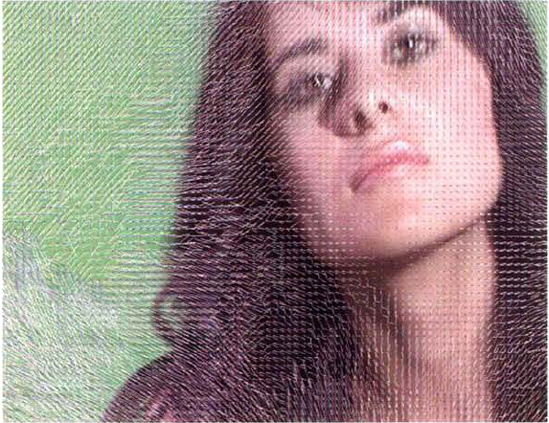
Figure 12.30. A detail of the motion vectors displayed by the OFlow node's Show Vectors parameter. A sample Nuke script is included as oflow.nk in the Tutorials folder on the DVD.
Additional quality parameters, including Smoothness, Block Size, Weight Red, Weight Green, and Weight Blue, work well with their default setting and should be adjusted only when problem solving. For additional information on these parameters, see the Nuke user guide.
Additional time-based nodes are included under the Time menu. A few are described in the following list:
FrameBlend and TimeEcho The FrameBlend node overlaps frames. You can select the number of adjacent frames to blend through the Number Of Frames cell. You can also select the Use Range check box and enter values into the Frame Range cells. If you select the Use Range check box, the result will not change over the duration of the timeline but will stay fixed. The FrameBlend node is useful for adding motion blur to objects that otherwise do not possess blur (see Figure 12.31). In addition, it provides a means to reduce or remove noise or grain from a plate shot with a static camera. The TimeEcho node produces results similar to FrameBlend, but it offers only three parameters. You can select the number of adjacent frames to blend through the Frames To Look At cell. The blending mode, set by the TimeEcho Method menu, includes Plus, Average, or Max options. If TimeEcho is set to Average or Plus, you can give greater blending weight to frames close to the current timeline frame by raising the Frames To Fade Out value.
FrameHold The FrameHold node repeats one frame of its input through the duration of the timeline. The Frame is determined by the First Frame parameter. However, if the Increment parameter value is raised above 0, First Frame is deactivated. Instead, every nth frame, as determined by Increment, is output. For example, if Increment is set to 5, Nuke holds frame 1 for frames 1 to 4, then holds frame 5 for frames 5 to 9, and so on.

The STMap node replaces input pixel values with values retrieved from a source input. The retrieval from the source input is controlled by the distortion channels of a distortion map. The distortion channels are labeled U and V where U determines the horizontal location of values within the source and V determines the vertical location of values within the source. Due to this functionality, it's possible to retexture a CG object in the composite (see Figure 12.32). In this situation, the distortion channels are derived from a UV shader render of the CG object. A UV shader converts UV texture coordinate values carried by the geometry into red and green colors.

Figure 12.32. (Top Left) Beauty pass of CG truck (Top Center) UV shader pass (Top Right) Dirt bitmap used for the source input (Bottom Left) STMap node in node network (Bottom Right) Resulting dirtied truck. A sample Nuke script is included as stmap.nk in the Tutorials folder on the DVD.
To use the STMap node in this fashion, it's necessary to create a high-quality UV shader render pass. Ideally, the pass should be rendered as a 32-bit float format, such as OpenEXR. Lower bit depths are prone to create noise when the texture is remapped. In addition, the UV render pass should be interpreted as Linear through the Colorspace menu of the Read node that imports it.
The STMap node, which is found in the Transform menu, has two inputs. The Src (source) input connects to the node that provides the new pixel colors. The Stmap input connects to the node carrying the distortion channels. For example, in Figure 12.32, a texture map featuring dirt is loaded into a Read node and connected to the Src input. A UV pass is loaded into a second Read node and is connected to the Stmap input. To establish which channels are used as distortion channels, the STMap node's UV Channels menu is set to Rgb. With this setting, the U is derived from the red channel and the V is derived from the green channel, as is indicated by Red and Green check boxes.
The STMap node does not process the alpha channel properly. Thus, it's necessary to retrieve the alpha by connecting a Copy node and a Premult node. In the Figure 12.32 example, the result is merged with the beauty render of the truck. When the STMap node is used, the truck can be dirtied without the need to re-render the CG sequence. In addition, the dirt map can be altered, updated, or replaced within the composite with little effort. The STMap node is able to remap a render even when the CG objects are in motion.
Nuke projects are called script files or scripts. Nuke also supports Python and TCL scripting. A scripting language is any programming language that allows a user to manipulate a program without affecting the program's core functions. As part of the scripting support, Nuke utilizes expressions and groups of nodes known as gizmos.
In Nuke, a gizmo is a group of nodes. Gizmos are useful for passing node networks from one artist to another or reapplying a proven node network to multiple shots on a single project. For example, the reformatting, color grading, and greenscreen removal sections of a node network may be turned into separate gizmos. A gizmo is stored as a text file with the .gizmo filename extension.

Figure 12.33. (Top) Group node network, as seen in the Groupn Node Graph tab (Bottom) The same Group node, as seen in the Node Graph tab
To create and save a gizmo, follow these steps:
Shift+select the nodes that you wish to include in a gizmo. In the Node Graph, RMB+click and choose Other → Group. A new Group node is created. The contents of the Group node are displayed in a new tab, which is named Groupn Node Graph (see Figure 12.33). In addition, Input and Output nodes are connected. The number of Input and Output nodes corresponds to the number of inputs and outputs that the originally selected nodes possessed.
Switch back to the Node Graph tab. Note that the new Group node is placed in the work area but is not connected to any other node. Nevertheless, the number of input and output pipes matches the input and output nodes in the Groupn Node Graph tab. The numbered pipe labels also correspond. For example, with the example in Figure 12.33, a node connection to the Group node's 2 input is actually a connection to the Scene1 node through the Input2 node.
Open the Group node's properties panel. Rename the node through the Name cell. To save the Group node as a gizmo, click the Export As Gizmo button.
A Group node has the same functionality as the originally selected nodes and can be connected to a preexisting node network. You can adjust the parameters of the original nodes without affecting the Group node or the duplicated nodes that belong to the group. If you want to adjust the Group node, switch back to the Group n Node Graph tab and open the properties panel for any contained nodes. To simplify the adjustment process, you can borrow knobs from the contained nodes and add them to the Group node (knobs are parameter sliders, check boxes, or cells). To do so, follow these steps:
Open the Group node's properties panel. RMB+click over the dark-gray area of the panel and choose Manage User Knobs. A Manage User Knobs dialog box opens (although the dialog box is labeled Nuke 5.1).
In the dialog box, click the Pick button (see Figure 12.34). In the Pick Knobs To Add dialog box, the nodes belonging to the Group node are listed. Expand the node or choice, highlight the knob name, and click OK. The knob, whether it is a slider, check box, or cell, is added to the Group node's properties panel under a new User tab. Repeat the process if you wish to add multiple knobs. To save the updated Group node as a gizmo, switch back to the Node tab of the properties panel and click the Export As Gizmo button.

Figure 12.34. (Top Box) Group1 node properties panel with Translate, Rotate, and Scale knobs borrowed from the Camera1 node (Center Box) Manage User Knobs dialog box with list of added knobs (Bottom Box) Pick Knobs To Add dialog box with list of nodes belonging to Group1 along with the nodes' available knobs
You can edit the added knob by clicking the Edit button in the Manage User Knobs dialog box. You have the option to change the knob's name, which is the channel name used for scripts and expressions. In addition, you can enter a new label, which is the word that appears to the left of the knob in the properties panel. You can also enter a ToolTip, which is the text that appears in a yellow box when you let your mouse pointer hover over the knob parameter in the properties panel. In fact, you are not limited to editing Group nodes, but can add or edit knobs for any node that appears in the Node Graph.
To open a preexisting gizmo, choose File → Import Script. The imported Gizmo node is named gizmon. Gizmo files are saved in a text format that contains a list of included nodes, custom parameter settings, custom knob information, and the node's XY position within the Node Graph.
Nuke supports the use of Python, which is a popular object-oriented programming language. To begin Python scripting, LMB+click a content menu button (see Figure 12.35) and choose Script Editor from the menu. By default, the editor opens as a pane on the left side. The lower, light-gray area of the editor is the Input window, while the darker, upper area is the Output window. To enter a script command, click the Input window so that it's highlighted and type or paste in the command. For example, you can type print "Hello there". To execute the script command, press Crtl+Enter. The result of the command is displayed in the Output window. A message following the phrase # Result will list whether the command was successfully or unsuccessfully carried out. If it was unsuccessful, a specific error is included.
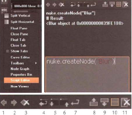
Figure 12.35. (Top Left) Script Editor option in a content button menu (Top Right) Script Editor with Output window at top and Input window at bottom (Bottom) Script Editor buttons, which include (1) Previous Script, (2) Next Script, (3) Clear History, (4) Source A Script, (5) Load A Script, (6) Save A Script, (7) Run The Current Script, (8) Show Input Only, (9) Show Output Only, (10) Show Both Input And Output, and (11) Clear Output Window
The Script Editor includes a number of menu buttons along the top of the Output window (see Figure 12.35). You can source, load, save, or execute by using the center buttons. Loading a script places it into the Input window but does not execute it. Sourcing a script executes the script immediately. Choosing the Save A Script button saves the script currently displayed in the Input window to a Python text file with a .py filename extension. To clear the contents of the Input window, click the Clear History button on the left. To clear the contents of the Output window, click the Clear Output Window button on the right.
Since Python is object oriented, it includes a wide array of objects. Objects, many of which are unique to Nuke, are collections or properties that perform specific tasks. Optionally, objects carry methods, which allow the object to operate in a different manner based on the specific method. The syntax follows object.method(value). Here are a few sample objects and methods (note that Python is sensitive to capitalization):
nuke.undo()andnuke.redo()execute an undo or a redo.nuke.getColor()launches the Get Color dialog box.nuke.createNode("name")creates a node and places it in the Node Graph.nameis the proper name of a node, such as Blur or Merge.nuke.message("text") pops up a dialog box with a message included between the quotes.nuke.plugins()lists currently loaded plug-ins with their paths.
To alter a node's parameter with Python, it's necessary to assign a variable to the node name. For example, entering gr=nuke.nodes.Grade() creates a Grade node and assigns it to a variable named gr. To alter one the of the Grade node's parameters, you can then enter gr["name"].setValue (value), where name lists the specific parameter. For example, you can enter gr["gamma"].setValue (1.5).
Variables are available for standard math operations. Python's math operators include + (add), - (subtract), (multiply), / (divide), and ** (powers, as in 2**10, or 210). For example, you can determine the memory usage in megabytes and gigabytes with the following lines:
mem=nuke.cacheUsage()
mb=mem/1024+.0
gb=mb/1024+.0
print "Kilobtyes:", mem
print "Megabtyes:", mb
print "Gigabytes:", gb
To enter a multiline command in the Script Editor, simply press the Enter key at the end of each command line. No special "end of line" symbol is necessary. In the preceding example,.0 is added to the end of the second and third line in order to convert the variable into a float (one that carries decimal places). If this is not done, the variables are assumed to be integers and the decimal places are dropped. As such, there are three variable types when working in Python. The variable type is determined when the variable is assigned a value:
test=100            integer
test=12.23          float
test="Finished"     string
if statements, which are a fundamental part of programming, are formatted in the following way (note that Python is sensitive to indentations):
if x==5:
   x=0
   print "X changed to 0"
elif x>5:
   x=10
   print "X changed to 10"
== is the same as "equals to." elif stands for "else if." In this example, if x is not equal to 5, it's passed to the elif portion of the statement. In turn, if x is not greater than 5, the if statement ends and x is not changed. if statements are a form of conditional that tests a variable a single time. To create a loop with Python, whereby a variable is tested repeatedly until the statement becomes false, use a while statement:
i=0
while i>10:
    i=i+1
    print "The value of i is", i
In this example, the third and fourth lines are repeatedly executed until i is no longer less than 10.
As demonstrated in Chapter 7, linking is the process by which two parameters are connected. Once they are linked, one parameter automatically inherits the values of the other. You can create a link by following these steps:
Place the mouse pointer over a parameter Animation button. Ctrl+LMB+drag the pointer to the Animation button of a second parameter. The two parameters can be derived from the same node or can be from two separate nodes.
If the second parameter is a valid choice, the mouse pointer will gain a small + symbol. Release the mouse button. A link is created. This is indicated by the parameter cell turning cyan and a green link pipe appearing between two nodes.
In reality, links are expressions, which are programmatic commands that relate two or more parameters. A destination parameter is "driven" by one or more source parameters, whereby the destination receives the source values.
Expressions rely on the naming convention node.parameter.child(frame). child is the subparameter, such as X, Y, Z or Red, Green, Blue. (frame) is optional and pulls a value as if the timeline was at a specific frame. For example, the Size parameter of a Blur node may be written as Blur1.size. At the same time, the Translate Y parameter of a Transform node may be written as Transform1.translate.y.
Aside from Ctrl+LMB+dragging between Animation buttons, you can create an expression with the following steps:
Select a destination parameter (one that will receive values from a source parameter). In the properties panel, RMB+click the destination parameter cell and choose Add Expression.
In the Add Expression dialog box, type the name of the source parameter. For example, type
Transform2.scale(see Figure 12.36). Click the OK button. A green link pipe is drawn between the destination and source nodes to indicate an expression exists. In addition, a green E symbol appears at the lower-right corner of the node that carries the destination parameter.
If the parameter name is mistyped or is invalid, ERROR appears beside the word Result in the Add Expression dialog box. Once the expression is successfully created, the destination parameter cell turns cyan. From that point forward, you can change the source value and the destination will automatically update.

Figure 12.36. (Top) Add Expression dialog box (Bottom) Green expression connection pipe drawn between two nodes
To delete an expression, RMB+click over the destination parameter cell and choose No Animation. To edit an expression, RMB+click and choose Edit Expression. You can add a mathematical operation to an expression using standard operators. For example, to make the destination parameter increase in value twice as fast as the source parameter, enter an expression that includes ×2 (for example, Transform2.rotate×2). Expression math can be fairly complex. For example, to rotate a car wheel automatically, you can use the Translate parameter of a car body with a formula similar to Transform1.translate.x × (360 / (6.28 × r)), where r is the screen radius of the wheel. In addition, a destination parameter can receive values derived from multiple source parameters. For instance, the expression Transform1.translate.x+Transform2.translate.y-Position1.translate.y(5) taps into three nodes. In this case, the Position1 node contributes the Translate Y value it possesses at frame 5.
Whereas Nuke supports Python, the program is actually built upon the TCL scripting language. TCL, short for Tool Command Language but pronounced "tickle," was developed in the late 1980s as an easily accessible language suitable for GUI creation. TCL scripts are often used in the following ways:
Adding functionality to nodes
Customizing the Nuke interface
Altering scripts based on environment variables
Reading/writing information from/to external databases
Analyzing the contents of scripts or specific node networks
You can enter a TCL command by choosing File → Script Command or pressing the X key (which is the default hot key). In the Script Command dialog box (see Figure 12.37), select the TCL check box, type the command, and click OK.

A few sample TCL commands are included here:
framenmoves the timeline to the declared frame.channelsnodelists all the channels carried by the named node.script_savefilenameandscript_save_asfilenamesave the script.expressionparameterreads a Nuke parameter and returns its value in a pop-up dialog box. For example, you can enterexpression Transform1.translate.x.setkeyparameter time valuesets a keyframe with a specific value for a specific frame for a particular parameter of a specific node. For instance, you can enter setkeyTransform1.rotate 10 1.5.connect_viewernumber nodeconnects a numbered, preexisting viewer to the named node.asktextpops up a Yes/No dialog box with a message defined by thetextvariable.
To execute a TCL command within the Script Editor Input window, use the Python nuke.tcl ("tcl") command. For example, enter nuke.tcl ("frame 20"). You can run a preexisting TCL script by choosing File → TCL File.
Jerry van der Beek received his master's degree in image and media technology from the Utrecht School of the Arts in the Netherlands. He went on to direct and animate several award-winning short films, including "Ja-Knikker" ("Oil Pumps"), "Jazz," and "The Car and the Road." Jerry worked his way up to animation director at Colossal Pictures, where he oversaw a number of successful ad campaigns. In 1996, he cofounded Little Fluffy Clouds with writer/producer Betsy De Fries.
Little Fluffy Clouds specializes in motion graphics and digital animation for television and online media. The studio is literally a two-person outfit that operates from a home studio on the edge of a national park in Marin County, California. Nevertheless, the studio has produced award-winning national spots for companies such asMercedes, Lexus, and McDonald's.

Jerry van der Beek at his workstation
(Little Fluffy Clouds uses the full line of Adobe products, including After Effects.)
LL: Since you work at a small studio, you have to be a jack-of-all-trades. Do you work on everything from the design to the delivery material?
JB: Yes. The 3D [animation], the Photoshop work... [W]e also do the initial design....
LL: What would be the advantages and disadvantages of being such a small outfit?
JB: There's not much second-guessing.... You become more like a small artist group with a real specific style instead of a company that does technical work. [W]e do design work, and we have the technical background to create it. [Unlike] big studios that actually hire external talent to design the spots, we are coming at it from the design aspect.
LL: In the last few years, there's been a convergence between 3D and 2D. Are there tasks that used to be the domain of 3D animation that you're now doing in the compositing program?
JB: [I]t's too cumbersome for a studio like us to delve into 3D. We have to have a really quick turn around.... I go for the look—you know, I want to sit in a package and dial things in—add a glow to it, make a certain core happen, see what the effect has in the entire shot....
LL: Does working in the composite give you greater flexibility?
JB: [S]ometimes...I want to have a certain kind of feeling, [so] let's open up the books and see what happens. I design [up] to a certain point, and then I make sure there's enough space there for a happy accident. And that's the great thing, also, of working in a small team.... I can do [the work] myself and say right away, "OK, I think this works and maybe we should steer the design a little more in this direction." So, in a small team, the process is much more organic.
LL: You work mainly with digital video source material. Do you prefer video over film?
JB: It depends.... [C]ommercials have a kind of graphic quality to them, [so] it's almost easier to integrate [video] because the footage already has a graphic quality.... But that, again, really depends on the design.
Tonya Smay graduated from the Rhode Island School of Design with a degree in film and video. She began her career in traditional animation by serving as a background painter, colorist, and effects animator for animated television shows such as "Doug" and "Dora the Explorer." She specialized in compositing and went on to freelance for various studios, including Curious Pictures, Brand New School, and Transistor Studios. At the time of this writing, Tonya was freelancing for Stardust Studios.

Tonya Smay in her home office
Stardust Studios is a creative production company specializing in motion graphics, animation, visual effects, and live-action production design for commercials, music videos, and in-store presentations. Stardust has offices in Santa Monica, California, and New York City. Recent clients include Adidas, AT&T, and BMW.
LL: While you were at school, did you learn compositing?
TS: I went to RISD for film and animation but barely used a computer at all. I did a lot of optical printing and was the teacher's assistant for the film effects class.... [I] barely used a computer. The methodology of optical printing is at the core of compositing—I'm just using a different instrument now.
LL: Aside from After Effects, which digital compositing packages have you used over the years?
TS: When I first started compositing, I had been working with traditional animators and cel (celluloid) painting. I started using Toonz software to digitally ink and paint the animators' drawings instead of using cels. The software was set up to scan animation paper and recognize the registration holes in the paper. You could then quickly ink and paint in large areas on hundreds of frames. Even the compositing part of Toonz looked like the tool of traditional animation: an exposure sheet. Toonz doesn't have all the third-party plug-ins that After Effects has. Also, it is so tightly structured for scanning traditional animation that I wouldn't use it in any other situation.
LL: How have high-definition formats affected the compositing process?
TS: The gains in speed made on the hardware side have been minimized due to the larger resolution images now commonly used—for example, HD.
LL: What resolution and bit depth do you normally composite at?
TS: 1920×1080. 16-bit.
LL: Is it common to work with 2.5D?
TS: I almost always work in 2.5D, even when I'm not working with [render] passes from a 3D program.
LL: What is the average time that you have to composite a project?
TS: Three weeks.
LL: Since you freelance and have the opportunity to work out of your home office periodically, what's the workflow like?
TS: [My] client postings (uploaded test renders, finished frames, and so on) are [at] strict dates and times. We have certain criteria to meet [at] each posting. After the posting, I'll receive a list of changes. [However, when I'm] in-house (at the studio), the approval process is much more fluid.... [T]he CD (creative director) stops by occasionally during the day or I'll call him over when I have something to show—a look for the scene or a problem solved.
LL: What type of workstation do you have in your home office?
TS: Right now, I'm using a quad-core Power PC G5 with 4 GB RAM, but I will be switching to an Intel Macintosh very shortly.
Chris Staves began his career as a Henry compositor for 525 Studios. After winning an MTV Music Video Award among other accolades, Chris left 525 to become a founding member of Method Studios L.A. (Method and R!OT merged in 2009). While at Method, Chris collaborated on such feature films as One Hour Photo and The Ring as well as an extensive number of commercials and music videos. In 2004, Chris opened MassMarket with Justin Lane. Chris currently serves as a Flame artist and creative director.
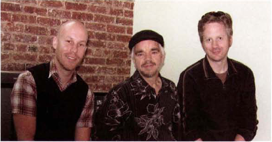
Justin Lane (left), Chris Staves (center), and Jeffrey Dates (right) in an in-house Flame bay
Justin Lane entered the visual effects field as a producer at Black Logic in New York. Thereafter, he collaborated with Method Studios on commercials for clients ranging from Nike to Acura and Xbox. In 2004, he opened MassMarket with Chris and continues to serve as executive producer.
Jeffrey Dates began his career at ReelFX in Dallas, Texas, where he served as a CG production artist and character animator. He later joined Janimation as creative director and CG lead. In 2007, Jeff moved to MassMarket as a VFX supervisor. At the time of this writing, Jeff was serving as a freelance animation director.
MassMarket is a VFX boutique and sister company of Psyop. Whereas Psyop directs commercial spots in-house, MassMarket works with outside directors and places an emphasis on photo-real visual effects. Recent work includes commercials for AT&T, Sprint, Nike, and Toyota. MassMarket and Psyop share facilities in Manhattan.
(MassMarket keeps six compositors on staff, although freelance artists are brought in for large projects.)
LL: You use After Effects as a secondary compositing program, but the Flame stations continue to do the brunt of the work. Do you see yourself moving more toward desktop compositing (programs that work on PCs or Macintoshes without the need for specialized hardware) in the future?
CS: We're trying to branch out more into desktop compositing—trying to use Nuke, but it's been difficult for us to make the transition.
JL: I think the reason studios that work on feature films have embraced Nuke is that they have time to set up a new pipeline. [They] can work out the kinks. For us, we have two weeks to do a job. If you throw somebody on Nuke, and it's not working, you have to figure out a solution [right away].
CS: Also, all the desktop solutions seem to be more shot-centric. They're just working on one shot at a time. Then you go into another software package, like Final Cut Pro, to work on your edit. In Flame, it's all integrated—you're doing the entire project, which is nice for a [studio that works closely with] clients. You can fix something really quickly, put it in the cut, see how it looks, and go back and forth without switching between applications.
Compositors hard at work on the first floor of the MassMarket / Psyop facility
LL: CG has advanced by leaps and bounds in the last few years. Do you find yourself working with all-CG spots, or is there still the need to use live-action footage and elements?
CS: Our philosophy is to try to get as much in-camera [as possible], whether that's working with prosthetics (visual effects makeup), or miniatures, or whatever it takes.... I think it's better to mix CG with live action. It hides the CG better.... It's harder in some ways because you have something [real] right there to compare the CG to. If you're trying to combine a CG car with a real car, the level of realism has to be that much higher. By the same token, by having some bits of realism in there, you're not really sure what's real and what's fake and what you've added and what you haven't added.... If clients come in and go, "We want to do it all CG," we're always a little wary. We'll go, "Can we shoot this?" or "Can we shoot that?"—even if it's just smoke or atmospheric elements....
JD: We're usually trying to re-create reality, so why not just shoot it. Real looks real.
LL: Do you think that compositing programs are advancing as fast as 3D programs?
CS: The biggest advances in compositing, at least in Flame, are picking up [tasks] that were traditionally done in CG. Being able to do projections, for instance....
As a final example of digital compositing, two composites created for Mercedes by Jerry van der Beek at Little Fluffy Clouds are included here. Aside from the CG car, which was rendered in Maya, all the elements were generated in After Effects with a combination of standard effects and a single additional plug-in (Trapcode Particular). These composites demonstrate that amazing visuals can be created within the compositing program by a single compositor.
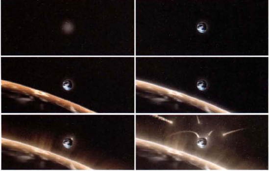
Six example steps of a composite featuring a planet approached by shooting stars (Images courtesy of Little Fluffy Clouds)

Six example steps of a composite featuring abstract light flares dancing around a car (Images courtesy of Little Fluffy Clouds)
Formal tutorials have not been included with this chapter. Instead, I'd like to encourage you to create your own unique projects using the source files included on this book's DVD along with the techniques discussed in this book's 12 chapters. There are almost endless possibilities with digital compositing, and no two compositors will produce the same results if set free with the same footage. In fact, if you come up with a unique composite using the resources from this book that you'd like to share, I'll post it on my website (www.BeezleBugBit.com). Just drop me at line at [email protected]. Have fun and good luck!
