
"I almost always work in 2.5D, even when I'm not working with [render] passes from a 3D program."
2D compositing is limited by its lack of depth. That is, the virtual camera can move in the X or Y direction but not along the z-axis. You can add the third dimension, however, by creating a 3D camera. In that case, 2D layers and outputs may be arranged in 3D space. This combination of 2D and 3D is often referred to as 2∼HFD or 2.5D. Both After Effects and Nuke support 2.5D workflows by making 3D cameras, lights, and materials available. Nuke goes so far as to add a complete set of shaders and geometry manipulation tools. With this chapter, you'll have the chance to set up a 2.5D environment complete with cameras, lights, materials, and texture projections.
By default, compositing programs operate in a 2D world. Layers and outputs of nodes are limited to two dimensions: X and Y. The ability of one layer or output to occlude another is based upon the transparency information of its alpha channel.
Compositing programs offer the ability to add the third dimension, Z, by creating or adding a 3D camera. The layers or outputs remain 2D, but they are viewable in 3D space. When a 2D image is applied to a plane and arranged in 3D space, it's commonly referred to as a card. Cards display all the perspective traits of 2D objects in 3D space (diminishing size with distance, parallel edges moving toward a vanishing point, and so on). Thus, once a card is in use, the compositing has entered 2.5D space. 2.5D, or 2∼HFD, is a name applied to a composite that is not strictly 2D or 3D but contains traits of both. 2.5D may encompass the following variations:
The ultimate goal of a 2.5D scene is to create the illusion of three-dimensional depth without the cost. The earliest form of 2.5D may be found in the multiplaning techniques developed by the pioneering animators at Fleischer Studios. With multiplaning, individual animation cels are arranged on separated panes of glass. (Cel is short for celluloid, which is a transparent sheet on which animators ink and paint their drawings.) The panes are positioned in depth below or in front of the camera. The cels are then animated moving at slightly different speeds. For example, a foreground cel is moved quickly from left to right, while the mid-ground cel is moved more slowly from left to right; the background painting of a distant landscape or sky is left static. The variation in speed creates the illusion of parallax shift. (See Chapter 10, "Warps, Optical Artifacts, Paint, and Text," for more information on parallax.) In addition, the assignment of cels to different glass panes allows the foreground cel to be out of focus. The combination of parallax approximation and real-world depth of field imparts a sense of three-dimensional depth to otherwise flat drawings.
You can replicate the multiplaning technique in a compositing program. For example, in Figure 11.1, a foreground layer, two mid-ground layers, and a background layer are arranged in After Effects. The foreground layer is blurred slightly and animated moving left to right. The mid-ground layers are animated moving more slowly in the same direction. The background layer is left static. In this example, the four layers were derived from a single digital photograph. Each layer was prepped in Photoshop and masked inside After Effects.
Although often successful, multiplaning is limited by the inability to move the camera off axis. That is, the camera must always point straight down the z-axis. Panning, tilting, or aggressively moving the camera about in 3D space will ruin the illusion of depth. However, if each layer of the multiplane is converted to a card and arranged in 3D space, the limitations are reduced. Using 2D cards in a 3D space is a common technique for visual effects work and is often employed to give depth to matte paintings and other static 2D backgrounds. For example, in Figure 11.2, cards are arranged to create a hallway. With this example, a single photo of a real hall is cut apart to create texture maps for each card. The gaps are only temporary; the final arrangement allows the cards to touch or slightly intersect. (See the After Effects tutorial at the end of this chapter for a demonstration of this technique.)
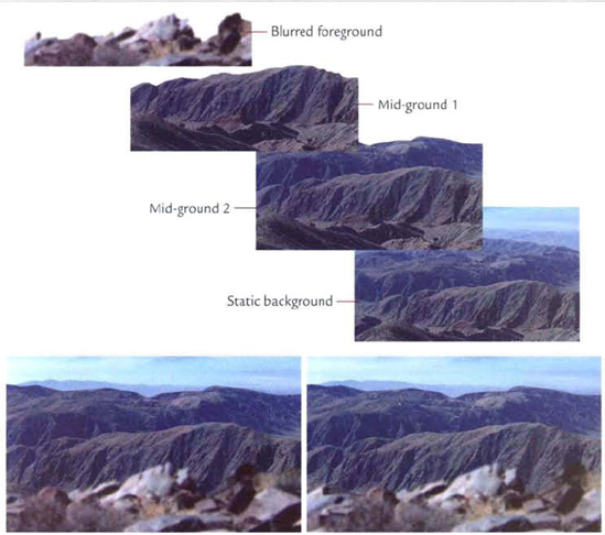
Figure 11.1. (Top) Four layers used to create multiplaning (Bottom Left) Resulting composite at frame 1 (Bottom Right) Resulting composite at frame 24. Note the shift in parallax. The foreground rocks are at a different position relative to the background. A sample After Effects project is included as multiplane.aep in the Tutorials folder on the DVD.
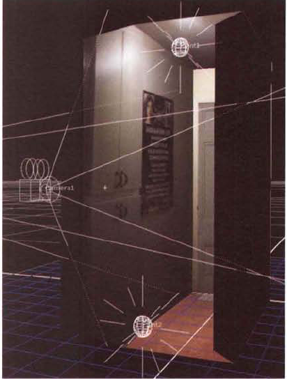
The use of cards in 3D space allows for greater movement of the camera. However, restrictions remain because excessive transforms in the X, Y, or Z direction will ruin the illusion. One way to reduce the limitations of cards is to project 2D images onto simple 3D geometry (see Figure 11.3). (See the Nuke tutorial at the end of this chapter for a demonstration of this technique.) The geometry may be imported from a 3D program, such as Maya, or may be constructed from 3D primitives provided by the compositing program (an ability of Flame, Inferno, and Nuke, for example). If physical measurements or laser scan information is collected from a live-action shoot, a location or set can be replicated as 3D geometry in exacting detail. In addition, such detailed information often includes the relative positions of the real-world camera and the real-world lights used to illuminate the scene. If the only reference available to the modeler is the captured film or video footage, the geometry may only be a rough approximation.
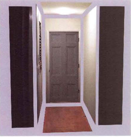
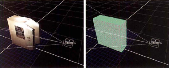
Figure 11.3. (Left) Image projected onto geometry through camera (Right) Wireframe of imported geometry
Ultimately, projections suffer the same limitations as the other 2.5D techniques. If the camera is moved too aggressively, the limited resolution of the projected image or the geometry itself may be revealed.
Once again, it's important to remember that the goal of a 2.5D scene is to create the illusion of three-dimensional depth without the necessity of rendering all the elements in 3D. Hence, in many situations, 2.5D techniques are perfectly acceptable when you're faced with scheduling and budgeting limitations. When successfully employed, 2.5D is indistinguishable from 3D to the average viewer.
After Effects and Nuke support 3D cameras, lights, and materials, allowing for the set up of 2.5D scenes.
After Effects supplies several means by which to convert a 2D layer into a 3D layer, thus making it a card. In addition, the program provides 3D cameras and 3D lights that let you work with a full 3D environment.
As described in Chapter 5, "Transformations and Keyframing," you can convert any After Effects layer into a 3D layer. You can do so by toggling on the 3D Layer switch for a layer in the layer outline or choosing Layer → 3D Layer. Once the layer is converted to 3D, you are free to transform, scale, or rotate the layer in the X, Y, or Z direction. However, the virtual camera used to view the 3D layer remains fixed. You can create a 3D camera, however, by following these steps:
Create a composition with at least one layer. Select the layer and choose Layer → 3D Layer. The 3D transform handle appears in the viewer. A 3D camera is functional only if a 3D layer exists.
Choose Layer → New → Camera. The Camera Settings dialog box opens (see Figure 11.4). Choose a lens size from the Preset menu. The lenses are measured in millimeters and are roughly equivalent to real-world lenses. Click the OK button.
A new 3D camera is created and is named Camera 1. The camera receives its own layer in the layer outline. However, the camera is not immediately visible in the viewer. The Composition panel, by default, shows a single view through a single viewer. You can switch to other views by changing the Select View Layout menu from 1 View to 4 Views (see Figure 11.5). The 4 Views option displays four views that correspond to top (XZ), front (XY), and right (XZ) cameras, plus the active perspective camera. Note that you can change a view by selecting the corresponding viewer frame (so that its corners turn yellow) and changing the 3D View Popup menu to the camera of your choice (see Figure 11.5). In addition, you can change the Magnification Ratio Popup menu for the selected view without affecting the other views.
You can translate the 3D camera by interactively LMB+dragging the camera body icon or camera point-of-interest icon in a viewer (see Figure 11.6). (The camera layer must be selected in the layer outline for the camera icons to be fully visible.) You can rotate the selected camera by interactively using the Rotate tool (see Figure 11.5). You can also adjust and keyframe the camera's Point Of Interest, Position, Orientation, and Rotation properties through the camera layer's Transform section in the layer outline.
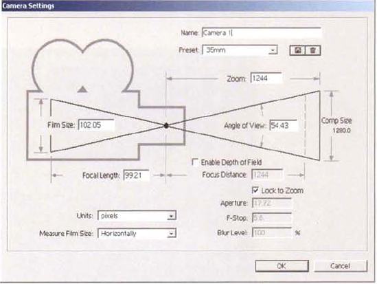
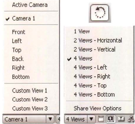
Figure 11.5. (Left) 3D View Popup menu (Top Right) Rotate tool (Bottom Right) Select View Layout menu
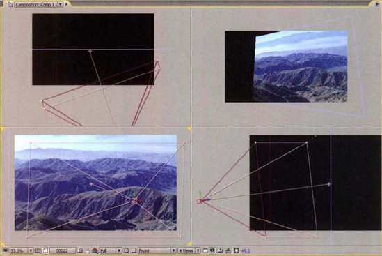
Figure 11.6. Composition panel set to 4 Views. The camera's body and point-of-interest icons are visible. Note that the yellow corners of the front view indicate that a particular viewer is selected.
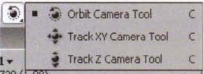
If you need to reframe a view, select the Orbit Camera, Track XY Camera, or Track Z Camera tool and LMB+drag in the corresponding viewer (see Figure 11.7). Orbit Camera rotates the 3D camera around the camera's point of interest. (You can only use the Orbit Camera tool in a perspective view.) Track XY Camera scrolls the view left/right or up/down. Track Z Camera zooms in or out.
After Effects is able to import camera data from a Maya scene file. However, special steps must be taken to ensure the successful importation. The steps include:
In Maya, create a non-default perspective camera. Animate the camera. Delete any static animation channels. Bake the animation channels by using the Bake Simulation tool. Baking the channels places a keyframe at every frame of the timeline.
In Maya, set the render resolution to a size you wish to work with in After Effects. It's best to work with a square-pixel resolution, such as 1280×720. Export the camera into its own Maya ASCII (
.ma) scene file. A sample scene file is included ascamera.main the Footage folder on the DVD.In After Effects, import the Maya ASCII file through File → Import. The camera data is brought in as its own camera layer in a new composition. The Position and XYZ Rotation properties of the layer are automatically keyframed to maintain the animation. The Zoom property is set to match the focal length of the Maya camera.
To look through the imported camera, set the 3D View Popup menu to the new camera name. If need be, add a 3D layer to the composition. To see the camera icon in motion, change the Select View Layout menu to 4 View and play the timeline.
If the camera is at 0, 0, 0 in Maya world space, it will appear at the top-left edge of the After Effects viewer when the view is set to Front or Top. Hence, it may be necessary to correct the imported camera animation by editing the keyframes in the Graph Editor or parenting the camera layer to a layer with offset animation.
After Effects also supports the importation of Maya locators (null objects that carry transformations). For more information, see the "Baking and Importing Maya Data" page in the After Effects help files.
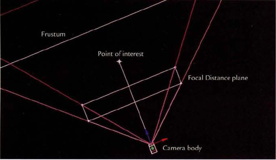
3D cameras in After Effects carry built-in depth of field. To activate this feature, toggle on the Depth Of Field property in the layer outline. The Focus Distance property, which is measured in pixels, sets the center of the focal region. The Focal Distance plane is represented as a subdivision in the camera icon's frustum, which is the pyramidal shape representing the camera's field of view (see Figure 11.8). The Aperture property establishes the camera's virtual iris size and f-stop. Higher Aperture values widen the iris and reduce the f-stop, thus leading to a narrower depth of field. The Blur Level property sets the degree of blurriness for regions outside the focal region. To reduce the strength of the blur, reduce the Blur Level value. The F-Stop property is accessible through the Layer → Camera Settings dialog box. If you manually change the F-Stop value, the Aperture value automatically updates.
A single composite can carry multiple 3D layers and cameras. Here are a few guidelines to keep in mind:
If you create a new layer by LMB+dragging footage from the Project panel to the layer outline, the new layer will remain a 2D layer. In fact, it will appear in every view as if fixed to the camera of that view. Once you convert it to a 3D layer, however, it will appear in the 3D space as a card.
To move a 3D layer, select the layer in the layer outline and interactively LMB+drag the corresponding card in a viewer. You can also adjust the layer's Transform properties, which include Position, Scale, Orientation, and Rotation.
3D layers support alpha channels. Shadows cast by the 3D layers accurately integrate the transparency.
A quick way to open the Camera Setting dialog box is to double-click the camera layer name. By default, camera distance units are in pixels. However, you can change the Units menu to Inches or Millimeters if you are matching a real-world camera.
You can activate motion blur for a 3D layer by toggling on the Motion Blur layer switch in the layer outline. By default, the blur will appear when the composite is rendered through the Render Queue. However, if you toggle on the Motion Blur composition switch (at the top of the Timeline panel), the blur will become visible in the viewer. The quality of the motion blur is set by the Samples Per Frame property, which is located in the Advanced tab of the Composition Settings dialog box. Higher values increase the quality but slow the viewer update. In contrast, the quality of motion blur applied to non-3D compositions is determined by the Adaptive Sample Limit property (the number of samples varies by frame with the Adaptive Sample Limit setting the maximum number of samples).
When you render through the Render Queue, the topmost camera layer in the layer outline is rendered. Camera layers at lower levels are ignored.
As soon as a layer is converted into a 3D layer, it receives a Material Options section in the layer outline. These options are designed for 3D lights. To create a light, follow these steps:
Select a layer and choose Layer → 3D Layer. The 3D transform handle appears in the viewer. A light is functional only if a 3D layer exists.
Choose Layer → New → Light. In the Light Settings dialog box, choose a light type and intensity and click the OK button. A new light is added to the composition and receives its own layer in the layer outline. A light illuminates the 3D layer. Areas outside the light throw are rendered black.
You can manipulate the light by interactively LMB+dragging the light body icon or light point-of-interest icon in a viewer. (The light layer must be selected in the layer outline for the light icons to be fully visible.) You can rotate the selected light by interactively using the Rotate tool. You can also adjust and keyframe the light's Point Of Interest, Position, Orientation, and Rotation properties through the Transform section of the layer outline.
You can readjust the light's basic properties by selecting the light layer and choosing Layer → Light Settings. There are four light types you can choose from:
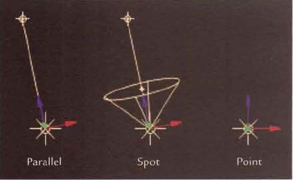
Parallel creates parallel rays of light that replicate an infinitely far source. The icon is composed of a spherical origin and a line extending to the point of interest (see Figure 11.9). You must "aim" the light by rotating the origin or positioning the point of interest. The position of the entire light icon does not affect the light quality. Direct lights are appropriate for emulating the sun or moon.
Spot creates a classic spot light with a light origin and cone. The origin is represented by a small sphere (see Figure 11.9). By default, the edge of the cone produces a hard, circular falloff. You can adjust the cone through the light's Cone Angle and Cone Feather properties.
Point creates an omni-directional light emanating from the center of its spherical icon (see Figure 11.9). Point lights are equivalent to incandescent light bulbs. Point lights have a Position property but no point of interest.
Ambient creates a light that reaches all points of the 3D environment equally. Hence, an ambient light does not produce an icon for the viewer and does not include a Transform section within its layer. Only two properties are available with this light type: Intensity and Color.
You can access the following properties through the Light Options section of the layer outline:
Intensity determines the brightness of the light.
Color tints the light.
Cone Angle and Cone Feather control the diameter and softness of light's cone if Light Type is set to Spot.
Casts Shadows allows cards to cast shadows onto other cards if toggled on (see Figure 11.10).
Shadow Darkness sets the opacity of the cast shadows.
Shadow Diffusion sets the edge softness of the cast shadows. High values slow the composite significantly.
Once a light exists, the properties within the Material Options section of the 3D layer take effect. A list of the Material Options properties follows:
Casts Shadows determines whether the 3D layer casts shadows onto other 3D layers. If Casts Shadows is set to Only, the layer is hidden while the shadow is rendered.
Light Transmission, when raised above 0%, emulates light scatter or translucence whereby light penetrates and passes through the 3D layer (see Figure 11.11).
Accepts Shadows determines whether the 3D layer will render shadows cast by other 3D layers.
Accepts Lights determines whether the 3D layer will react to 3D lights. If toggled off, the footage assigned to the layer is rendered with all its original intensity. Accepts Lights has no effect on whether the 3D layer receives shadows, however.
Diffuse represents the diffuse shading component—the lower the value, the less light is reflected toward the camera and the darker the 3D layer. (For more information on shading components, see Chapter 9, "Integrating Render Passes.")
Specular controls the specular intensity. The higher the value, the more intense the specular highlight (see Figure 11.12).
Shininess sets the size of the specular highlight. Higher values decrease the size of the highlight.
Metal controls the contribution of the layer color to the specular highlight color. If Metal is set to 100%, the specular color is derived from the layer color. If Metal is set to 0%, the specular color is derived from the light color. Other values mix the layer and light colors.
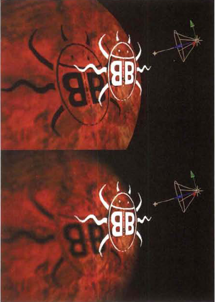
Figure 11.10. (Top) A spot light casts a shadow onto a 3D layer with a red abstract image. A second 3D layer, with the bug logo, carries transparency through an alpha channel. The light's Cone Feather and Shadow Diffusion are set to 0. (Bottom) Same setup with Cone Feather set to 35% and Shadow Diffusion set to 15. A sample After Effects project is included as shadow.aep in the Tutorials folder on the DVD.
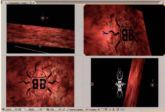
Figure 11.11. A point light is placed behind the 3D layer with a red abstract image. Because the layer's Light Transmission property is set to 100%, the light penetrates the surface and reaches the camera. The 3D layer with the bug logo has a Light Transmission value of 0% and thus remains unlit from the front. A sample After Effects project is included as transmission.aep in the Tutorials folder on the DVD.

Figure 11.12. (Left) 3D layer lit by a point light. Diffuse, Specular, Shininess, and Metal properties are set to 100%. (Right) Same setup with Diffuse set to 70%, Specular set to 40%, Shininess set to 5%, and Metal set to 50%. A sample After Effects project is included as specular.aep in the Tutorials folder on the DVD.
Nuke supplies a comprehensive 3D environment for working with cards, 3D cameras, 3D lights, and imported geometry. At its simplest, the 3D environment requires the following nodes to operate:
Camera creates a 3D camera and defines the 3D projection used by the renderer.
Card is a primitive plane that carries the 2D input.
Scene groups together 3D lights and geometry, such as planes created by Card nodes. This node is fed into the ScanlineRender node.
ScanlineRender provides a default renderer for use with the 3D environment. The 3D environment must be rendered out as a 2D image before it can be used as part of a non-3D node network.
To set up a 3D environment, follow these steps:
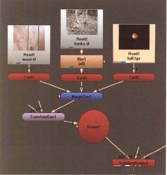
In the Node Graph, RMB+click and choose Image → Read. Choose a file or image sequence through the Read node's properties panel. With the Read1 node selected, choose 3D → Geometry → Card. With the Card1 node selected, choose 3D → Scene.
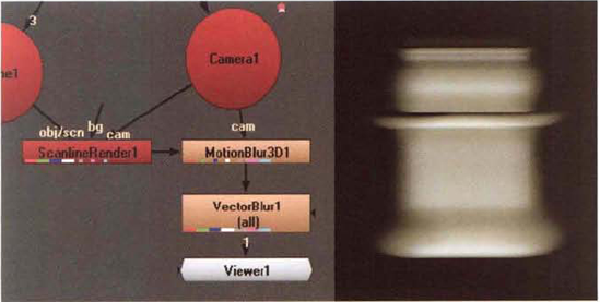
With no nodes selected, chose 3D → Camera. With no nodes selected, choose 3D → ScanlineRender. Connect the Obj/Scn input of the ScanlineRender1 node to the Scene1 node. Use Figure 11.13 as a reference. Connect the Cam input of the ScanlineRender1 node to the Camera1 node. Connect a viewer to the ScanlineRender1 node.
Once you set up a 3D environment, you can view it with a standard viewer. To do so, change the View Selection menu, at the upper right of the Viewer pane, to 3D (see Figure 11.14). Because the camera and card are created at 0, 0, 0 in 3D world space, the card is not immediately visible. Change the Zoom menu, directly to the left of the View Selection menu, to Fit.
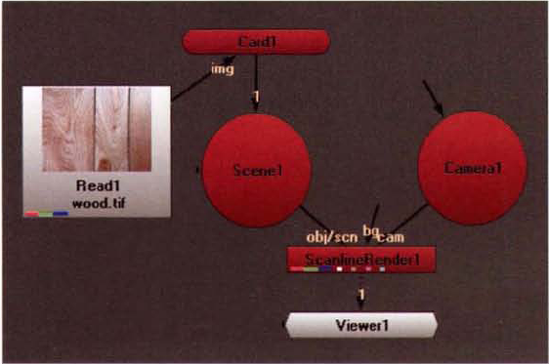
Figure 11.13. Node network of a 3D environment. A sample Nuke script is included as simple_3D.nk in the Tutorials folder on the DVD.
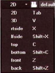
You can select specific orthographic views by changing the View Selection menu to Top, Bottom, Front, Back, Lfside, or Rtside. If you set the View Selection to 3D, you can orbit around the origin by Alt+RMB+dragging. You can scroll by Alt+LMB+dragging in any of the views. You can zoom by Alt+MMB+dragging in any of the views. To return the viewer to the point of view of the camera, change the View Selection menu back to 2D. (If the camera intersects the card, translate the camera backward.)
The 3D camera is represented by a standard icon that includes the camera body and frustum (pyramidal shape that represents the field of view). You can interactively move the camera in the viewer by selecting the Camera node or by clicking the camera icon (see Figure 11.15). Once the camera is selected, you can LMB+drag an axis handle that appears at the base of the lens. To rotate the camera, Ctrl+LMB+drag. (You must keep the properties panel open to manipulate the camera interactively.) In addition, the Camera node's properties panel contains a full set of transform parameters, which you can change by hand and animate via corresponding Animation buttons. You can change the camera's lens by entering a new Focal Length value in the Projection tab.
You can transform a Card node in the same manner as a Camera node. Once the Card node is selected, a transform handle appears at its center.
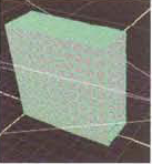
A Card node is only one of four primitive geometry types available through the 3D → Geometry menu. Each type carries an Img input, which you can use to texture the geometry. However, each type treats the texture mapping in a different way:
Cube applies the Img input to each of its six sides.
Cylinder stretches the Img input as if it were a piece of paper rolled into a tube. By default, the cylinder has no caps. You can force a top or bottom cap by selecting the Close Top or Close Bottom check box in the node's properties panel. With caps, the top or bottom row of pixels is stretched to the center of the cap.
Sphere stretches the Img input across its surfaces, pinching the top and bottom edge of the image into points at the two poles.
If you create more than one piece of geometry, you must connect each piece to a Scene node, which in turn must be connected to a ScanlineRender node. The connections to a Scene node are numbered 1, 2, 3, and so on. If a piece of geometry is not connected to a Scene node, it remains visible in the 3D view of the viewer but will not appear in the 2D view of the viewer. Again, the 2D view, set by the View Selection menu, represents the view of the camera and the ultimate output of the ScanlineRender node.
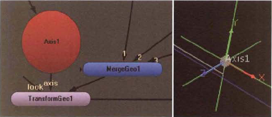
You can interactively scale, rotate, or translate the geometry of a Cube, Card, Cylinder, or Sphere node. You can group multiple pieces of geometry together by connecting their outputs to a MergeGeo node (in the 3D → Modify menu). To transform the resulting group, connect the output of the MergeGeo node to a TransformGeo node (in the 3D → Modify menu). See Figure 11.16 for an example. When the TransformGeo node is selected, a single transform handle appears in the viewer. The TransformGeo node's properties panel contains all the standard transform parameters, which you can adjust and animate.
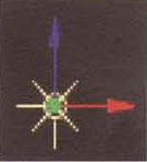
The TransformGeo node includes two inputs with which you can constrain the group: Look and Axis. You can connect the Look input to a geometry or light node. This forces the TransformGeo node always to point its local z-axis toward the connected object. You can also connect the Look input to a Camera or second TransformGeo node that is not part of the same node network. On the other hand, you can connect the Axis input to an Axis node. An Axis node (in the 3D menu) carries a transformation without any geometry. When an Axis node is connected to the Axis input, it serves as a parent node and the TransformGeo node inherits the transformations. If the Axis node is located a significant distance from the TransformGeo node, the geometry connected to the TransformGeo node will suddenly "jump" to the Axis location. The Axis node is represented in the viewer as a six-pointed null object (see Figure 11.17).
The ReadGeo node is able to import polygonal OBJ and FBX files. UV information survives the importation. To apply the node, follow these steps:
With no nodes selected, RMB+click and choose 3D → Geometry → ReadGeo. Open the ReadGeo node's properties panel. Browse for an OBJ or FBX file through the File parameter. A sample OBJ file is included as
geometry.objin the Footage folder of the DVD. A sample FBX file is included asgeometry.fbx. If there is more than one geometry node in an FBX file, set the Node Name menu to the node of choice. Connect the output of the ReadGeo node to the Scene node currently employed by the 3D environment. The imported geometry appears in the viewer.If you are opening an FBX file and wish to import the node's animation, set the Take Menu to Take 001 or the take of your choice. If takes were not set up in the 3D program, Take 001 will hold the primary animation.
To texture the geometry, connect a Read node to the Img input of the ReadGeo node. Load a texture file into the Read node. A sample texture file, which matches
geometry.obj, is included astexture.tgain the Footage folder on the DVD. If you switch to the 2D view of the viewer (which is the camera's point of view), geometry that carries UV information will display its texture by default (see Figure 11.18). At this stage, however, the surface will not possess any sense of shading. To add shading, you must connect a shader node and add at least one 3D light (see the sections "Creating 3D Lights" and "Adding Shaders" later in this chapter). If you switch to the 3D view of the viewer, the geometry is also textured by default. To display a wireframe version, change the ReadGeo node's Display menu to Wireframe.
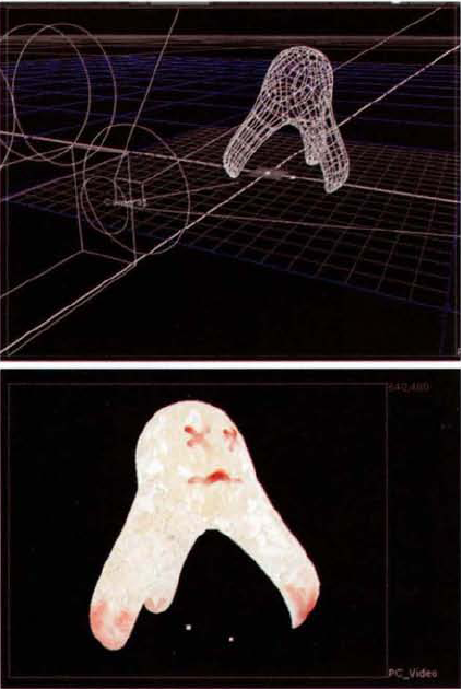
Figure 11.18. (Top) Imported OBJ geometry, as seen in wireframe in the 3D view of the viewer (Bottom) Textured geometry, as shown in the 2D view of the viewer. A shader and light node must be added to give a sense of shading.
The WriteGeo node exports geometry as an OBJ file when its Execute button is clicked. If the WriteGeo node's input is connected to a geometry node, the exported OBJ carries no transformation information. If you connect the WriteGeo node's input to a TransformGeo node, the exported OBJ inherits the transformation information as it stands for frame 1. If you connect the WriteGeo node's input to a Scene node, the exported OBJ includes all the geometry connected to the Scene node. Before you can use the Execute button, however, you must select a filename through the File parameter. Include the .obj extension for the exportation to work. Once you click the Execute button, the Frames To Execute dialog box opens. Despite this, the node can accept a frame range of only 1, 1.
You can light geometry within Nuke's 3D environment with the 3D → Lights menu. Once a light node is created, its output must be connected to a Scene node for its impact to be captured by the camera. The available light types follow:
Light creates a point light icon by default, but it is able to emulate three styles of lights through its own Light Type menu. These include point, directional, and spot. Each style of light functions in a manner similar to the Point, Direct, and Spot nodes. The Light node supports the ability to import lights through an FBX file, which is described in the section "Importing and Exporting Data" later in this chapter.
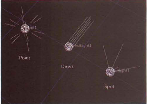
Point creates an omni-directional light emanating from the center of its spherical icon (see Figure 11.19). Point lights are equivalent to incandescent light bulbs.
Direct creates parallel rays of light that replicate an infinitely distant source. The icon is a small sphere with lines extending in one direction (see Figure 11.19). The lines indicate the direction of the light rays; hence, you must "aim" the light by rotating it. The light's position does not affect the light quality. Direct lights are appropriate for emulating the sun or moon.
Spot creates a classic spot light with a light origin and cone. The origin is represented by a small sphere, while the cone is represented by four lines extending outward (see Figure 11.19). The edge of the cone produces a hard, circular falloff. You can adjust the cone through the node's properties panel. The Cone slider controls the cone spread; valid ranges are 0 to 180°. The Cone Penumbra Angle slider sets the size of the cone's edge falloff. Negative values fade the cone from the edge inward. Positive values fade the cone from the cone edge outward. In contrast, the Cone Falloff slider determines how quickly the light intensity diminishes from the cone center to the cone edge. The higher the value, the more focused the light.
Environment uses a spherically mapped input to determine its intensity. The Environment node is designed for image-based lighting and is therefore discussed in more detail in Chapter 12, "Advanced Techniques".
All the light nodes share a set of parameters, which are described here:
Color allows the light to be tinted.
Intensity controls the strength of the light.
Falloff Type determines the light decay. By default, the light intensity does not diminish with distance. To create real-world decay, where the intensity is reduced proportionally with the square of the distance (intensity/distance2), set the menu to Quadratic. If you set the menu to Linear, the intensity diminishes at a constant rate and thus travels farther than it would with Quadratic. If you set the menu to Cubic, the decay is aggressive as the intensity is reduced proportionally with the cube of the distance (intensity/distance3).
Camera, geometry, and light mode's share a set of parameters:
Display allows you to change the node icon's appearance in the 3D view of the viewer. Menu options include Off (hidden), Wireframe, Solid (shaded), and Textured.
Pivot sets the XYZ position of the pivot point of the node (as measured from the node's default pivot location, which may be the volumetric center of geometry or the world origin). Scaling, rotations, and translation occur from the pivot. For example, if the pivot is set outside a geometry node, the geometry will rotate as if orbiting a planet.
Transform Order sets the order that the node will apply scale, rotate, and translation transformations. For example, SRT, which is the default setting, applies scaling before rotation or translation. The transform order can affect the transformation result if the object's pivot point is not volumetrically centered.
Rotation Order determines the order in which each axis rotation is applied to a node. Although the ZXY default is fine for most situations, the ability to change rotation order is useful for specialized setups.
Uniform Scale scales the object equally in all three directions. Uniform Scale serves as a multiplier to Scale XYZ. For example, if Scale XYZ is 0.5, 1, 0.2 and Uniform Scale is 2, the net result is a scale of 1, 2, 0.4.
Any light you add to the scene will illuminate the surface of the geometry. However, the geometry will appear flat unless you connect a shader. The 3D → Shader menu includes five basic shaders, any of which you can connect between the Img input of a geometry node and the output of the node providing the texture information:
Diffuse adds the diffuse component to a surface. The term diffuse describes the degree to which light rays are reflected in all directions. Therefore, the brightness of the surface is dependent of the positions of lights within the environment. The node only provides a White slider, which establishes the surface color.
Specular adds the specular component to the surface. A specular highlight is the consistent reflection of light in one direction. In the real world, a specular highlight results from an intense, confined reflection. In the realm of computer graphics, specular highlights are artificially constructed "hot spots." You can control the size of Nuke's specular highlight by adjusting the Min Shininess and Max Shininess sliders.
Emission adds the emissive or ambient color component to the surface. Ambient color is the net sum of all ambient light received by the surface in a scene. High Emission slider values wash out the surface. The Emission shader ignores all light nodes.
BasicMaterial and Phong combine the Diffuse, Specular, and Emission nodes. Phong has a slight advantage over BasicMaterial in that it calculates specular highlights more accurately. However, in many situations, the shading appears identical.
Each of the five shaders carries various inputs. The mapD input is designed for diffuse or color maps. The map may come in the form of a bitmap loaded into a Read node, a Draw menu node, or any other node that outputs useful color values (see Figure 11.20). The mapS input is designed for specular maps. The mapE input is designed for emissive (ambient color) maps. The mapSh input is designed for shininess maps. If a shader node has a Map input, the input represents the key component. For example, the Diffuse shader Map input represents the diffuse component, while the Emission shader Map input represents the emissive component.
If you wish to merge two shaders together, use the MergeMat node (in the 3D → Shader menu). For example, connect a Specular node to input A of a MergeMat node (see Figure 11.21). Connect a Diffuse node to input B of the MergeMat node. Connect the output of the MergeMat node to the Img input of the geometry node. The MergeMat node's Operation menu determines the style of merge. When combining a Diffuse and Specular node, set the Operation menu to Plus.
You can also chain an unlimited number of shader nodes together by connecting the output of one to the unlabeled input of the next (see Figure 11.21). Since the outputs are added together, however, this may lead to an overexposed surface unless the shader properties are adjusted.

Figure 11.20. (Left) A specular map is connected to the mapS input of a Phong node. A diffuse (color) map is connected to the mapD input. (Bottom Right) The resulting camera render. A sample Nuke script is included as shaded.nk in the Tutorials folder on the DVD.
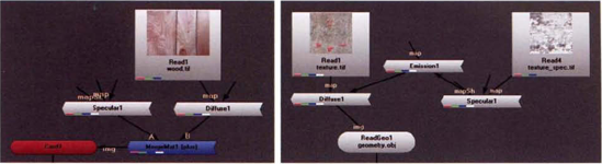
Figure 11.21. (Left) A MergeMat node is used to combine Specular and Diffuse shader nodes. A sample Nuke script is included as mergemat.nk in the Tutorials folder. (Right) Diffuse, Emission, and Specular shaders are chained through their unlabeled inputs. A sample Nuke script is included as shader_chain.nk in the Tutorials folder on the DVD.
The 3D → Modify menu includes a number of nodes designed to manipulate geometry. UVProject, Normals, and DisplaceGeo are described in the following sections.
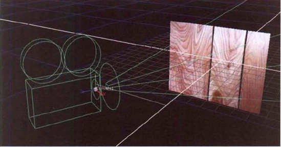
The UVProject node projects an image onto a piece of geometry while overriding the geometry's inherent UV values. To apply the node, follow these steps:
With no nodes selected, RMB+click and choose 3D → Modify → UVProject. LMB+drag the UVProject node and drop it on top of the connection line between a geometry or MergeGeo node and its corresponding Scene node (see Figure 11.22).
Connect an Axis node to the Axis/Cam input of the UVProject node. As soon as the connection is made, the projection functions and is visible in the viewer (see Figure 11.22). (This assumes that the geometry node's Display and Render menus are set to Textured).

Figure 11.22. (Left) Card and Sphere nodes are combined with a MergeGeo node. The MergeGeo node's UV texture space is provided by a UVProject node with an Axis node supplying the projection coverage information. (Top Right) Resulting render with Projection set to Planar. (Bottom Right) Resulting render with Projection set to Cylinder. A sample Nuke script is included as uvproject.nk in the Tutorials folder on the DVD.
You can also attach a new Camera node to the Axis/Cam input. You can create a new Camera or Axis node for the sole purpose of working with the UVProject node. If you connect an Axis node, the projection coverage is based upon the node's Translate, Rotate, and Scale parameter values. If you connect a Camera node, the projection coverage is based upon the node's Translate, Rotate, Scale, Horiz Aperture, Vert Aperture, and Focal Length parameter values. As you change the various parameters, the projection updates in the viewer. If the Scale value is too small, the edge pixels of the texture are streaked to fill the empty area of the surface.
The UVProject node carries four projection types, which you can access through the Projection menu. If you set the menu to Planar, the projection rays are shot out in parallel. Planar is suitable for any flat surface. If you set the menu to Spherical, the input image is wrapped around a virtual sphere and projected inward. Spherical is suitable for geometry representing planets, balls, and the like. If you set the menu to Cylinder, the projection is similar to Spherical; however, it is less distorted than the Spherical projection because it does not pinch to the input image edges along the top and bottom. The default menu setting, Perspective, projects from the view of the node. Thus the Perspective setting is the most appropriate if a Camera node is connected. Note that the Focal Length, Horiz Aperture, and Vert Aperture parameters of the Camera node affects the projection only if the UVProject node's Projection menu is set to Perspective.
The Project3D node (in the 3D → Shader menu) can produce results similar to the UVProject node. However, its application is slightly different:
With no nodes selected, RMB+click and choose 3D → Shader → Project3D. LMB+drag the Project3D node and drop it on top of the connection line between a shader node and a geometry node. For a texture map to be projected, a Read node with the texture map must be connected to the appropriate map input of the shader node.
Connect a Camera node to the Cam input of the Project3D node. As soon as the connection is made, the projection functions and is visible in the viewer (so long as the geometry's Display and Render menus are set to Textured). The orientation of the camera frustum determines the projection coverage. If the connected Camera node is positioned in such a way that the frustum coverage is incomplete, the uncovered part of the surface will render black.
With the Normals node, you can manipulate the normals of primitive or imported polygon geometry. To utilize the node, place it between the geometry node and the corresponding Scene node. For the results of the node to be seen, the Img input of the geometry node must be connected to a shader node. The Invert check box, beside the Action menu, flips the normals by 180°. The Action menu supports the following options:
Set orients all normals along a vector established by the Normal XYZ cells. If the Normal XYZ values are 0, 0, 0, the normals are "set to face," which facets the resulting render. If the Normal XYZ values are non-default values, the normals are oriented in the same direction. For example, if the camera is looking down the –z-axis, which is the default, you can set the Normal XYZ cells to 0, 0, 1 and thus have all the normals point toward the camera (this creates a flat-shaded "toon" result).
Build determines how smoothly the surface is rendered across adjacent polygons (see Figure 11.23). If the Angle Threshold slider is set to 0, no smoothing occurs and the surface appears faceted. If Angle Threshold is set above 0, only adjacent polygons that possess an angle less than the Angle Threshold value are smoothed. The angle is measured between the normals that exist at shared vertices of the corner of two adjacent faces. A slider value of 180 smooths all the polygons.
Lookat points all the surface normals toward the node that is connected to the Normals node's Lookat input. For Lookat to function in an expected fashion, Normal XYZ must be set to 0, 0, 0.
Delete removes a particular surface attribute. The attribute is established by the Attr Name cell, which uses code. N stands for normal, uv stands for UV points, and so on. For a complete list of attributes, hover the mouse pointer over the cell.
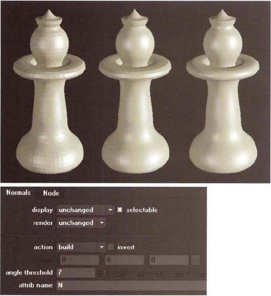
Figure 11.23. (Top Left) Geometry with Action menu set to Build and Angle Threshold set to 0 (Top Center) Angle Threshold set to 7. Note the faceting that remains around the central collar. (Top Right) Angle Threshold set to 180 (Bottom) Properties panel of the Normals node. A sample Nuke script is included as normals.nk in the Tutorials folder on the DVD.
The DisplaceGeo node displaces the surface of a geometry node by pulling values from an input. The input may be any node that outputs color values. For example, you can connect the DisplaceGeo node's Displace input to a Checkerboard node or a Read1 node that carries a texture map. (The DisplaceGeo node is placed between the geometry node and the corresponding Scene node.) The strength of the displacement is controlled by the Scale slider. To soften the displacement, increase the Filter Size value. By default, the displacement is based on luminance, but you can change the Source menu to a particular channel. If you wish to offset the resulting displacement in space, adjust the Offset XYZ values.
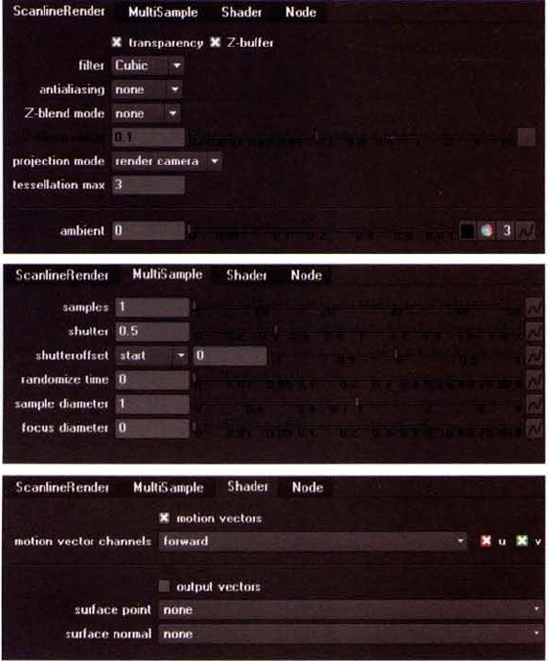
Initially, the ScanlineRender node produces poor results in the 2D view of the viewer. You can improve the render quality through the node's various parameters. The following are found in the ScanlineRender tab of the node's properties panel:
Filter applies the standard set of convolution filters to the render to avoid anti-aliasing issues.
Antialiasing, when set to Low, Medium, or High, reduces or prevents stairstepping and similar aliasing artifacts at surface edges and surface intersections.
Z-Blend Mode controls how intersecting surfaces are blended together along the intersection line. If the menu is set to None, a hard edge remains. If the menu is set to Linear or Smooth, a smoother transition results. The distance the blend travels along each surface is set by the Z-Blend Range slider (see Figure 11.24).
Additional parameters are available through the MultiSample tab:
Samples sets the number of subpixel samples taken per pixel. The higher the Samples value, the more accurate the result will be and the higher the quality of the anti-aliasing. If Samples is set to a high value, you can leave the Antialiasing menu, in the ScanlineRender tab, set to None.
Shutter and Shutter Offset determine motion blur length. See the "Tips & Tricks" note at the end of this section for information on the handling of motion blur.
Randomize Time adds jitter to the subpixel sampling. This prevents identifiable patterns from appearing over time. Unless you are troubleshooting aliasing artifacts, however, you can leave this set to 0.
Sample Diameter sets the filter kernel size for the anti-aliasing process. Values over 1 may improve the quality.
Any improvement to the render quality will significantly slow the update within the viewer. However, for acceptable results to be rendered through a Write node, high-quality settings are necessary.
You can import cameras, lights, and transforms from an FBX file through Nuke's Camera, Light, and Axis nodes. In addition, Nuke offers the Chan (.chan) file format for quickly importing and exporting animation data.
The Camera node can import an animated camera. For example, you can import a Maya camera with the following steps:
Open a Camera node's properties panel. Select the Read From File check box. This ghosts the transform parameters.
Switch to the File tab. Browse for an FBX file through the File parameter. A sample FBX file is included as
camera.fbxin the Footage folder on the DVD. A warning dialog box pops up. Click Yes. Any prior settings are destroyed for the Camera node with which you are working.The imported camera icon appears in the 3D view of the viewer. If the FBX file contains more than one camera, you can switch between them by changing the Node Name menu to another listed camera (see Figure 11.25). Note that the FBX format attaches a Producer suffix to default camera nodes, such as Producer Top. With the sample
camera.fbxfile, the custom camera is named Panavision.At this point, the camera's animation will not appear. To import the keyframes, change the Take Name menu to Take 001. If you did not set up takes in the 3D program, Take 001 will hold the primary animation. To see the camera in motion, switch the View Selection menu to 3D and play the timeline.
If you would like to transform the imported camera, return to the Camera tab and deselect the Read From File check box. The keyframes are converted to Nuke curves and are editable through the Curve Editor. In addition, the transform properties become available through the Camera tab.
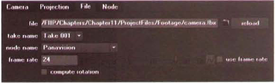
Aside from the transformations, Nuke is able to import the camera's focal length and the project's frames per second. You can force a different frame rate on the FBX file by changing the Frame Rate slider in the File tab.
The Light node can import a light from an FBX file. You can follow these steps:
Open a Light node's properties panel. Select the Read From File check box. This ghosts the transform parameters.
Switch to the File tab. Browse for an FBX file through the File parameter. A sample FBX file is included as
lights.fbxin the Footage folder on the DVD. A warning dialog box pops up. Click Yes. Any prior settings are destroyed for the Light node you are working with.The imported light icon appears in the 3D view of the viewer. Nuke will match the light type to the type contained with the FBX file. Nuke supports spot, directional, and point light types but is unable to read ambient lights. If the FBX file contains more than one light, you can switch between them by changing the Node Name menu to another listed light.
At this point, any animation on the imported light will not appear. To import the keyframes, change the Take Name menu to Take 001 (if you did not set up takes) or the take number of your choice.
If you would like to transform the imported light, return to the Light tab and deselect the Read From File check box. The keyframes are converted to Nuke curves and are editable through the Curve Editor. In addition, the transform properties become available through the Light tab.
Aside from the transformations, Nuke is able to import the light's intensity value and the project's frames per second. As you are importing the light, you can change the Frame Rate and Intensity Scale values through the File tab.
The Axis node can extract transformation information from a targeted node in an FBX file. Follow these steps:
Open an Axis node's properties panel. Select the Read From File check box. This ghosts the transform parameters.
Switch to the File tab. Browse for an FBX file through the File parameter. A sample FBX file is included as
transform.fbxin the Footage folder on the DVD. A warning dialog box pops up. Click Yes. Any prior settings are destroyed for the Axis node with which you are working.The Axis icon jumps to the same coordinates in space as the imported node. If the FBX file contains more than one node, you can switch between them by changing the Node Name menu to another listed node.
At this point, any animation will not appear. To import the keyframes, change the Take Name menu to Take 001 (if you did not set up takes) or the take number of your choice.
If you would like to transform the imported axis, return to the Axis tab and deselect the Read From File check box. The keyframes are converted to Nuke curves and are editable through the Curve Editor. In addition, the transform properties become available through the Axis tab.
Camera, Light, and Axis nodes support the Chan file format (.chan), which carries animated transform information. To import a Chan file, click the Import Chan File button and browse for the file. The imported transformation data is applied to the node and the animation curves are updated. To export a Chan file, click the Export Chan File button. Each Chan file is a text list that includes each frame in the animation sequence with transformation values for each animated channel. The ability to import and export the files allows you to transfer animation quickly from one node to another within the same script or different scripts.
The MotionBlur3D node, in the Filter menu, creates motion blur for cameras and objects moving within a 3D environment. It offers the advantage of a high-quality linear blur at relatively little cost. For the node to function, the outputs of the ScanlineRender node and the Camera node are connected to the MotionBlur3D node (see Figure 11.26). In turn, the output of the MoitonBlur3D node is connected to the input of the VectorBlur node. If the VectorBlur's UV Channels menu is set to Motion, the motion blur appears in the 2D view of the viewer.
In these tutorials, you'll have the opportunity to turn a 2D photo of a hallway into a 3D model within the composite.
By arranging 3D cards in 3D space, you can replicate a hallway.
Create a new project. Choose Composition → New Composition. In the Composition Settings dialog box, change the Preset menu to HDV/HDTV 720 29.97 and set Duration to 30. Import the following files:
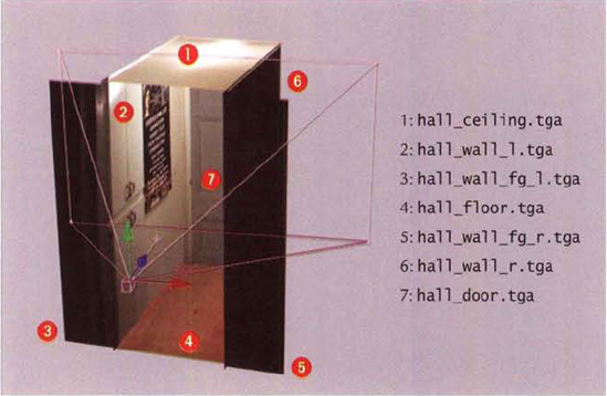
hall_wall_fg_l.tga
hall_wall_fg_r.tga
hall_wall_l.tga
hall_wall_r.tga
hall_ceiling.tga
hall_floor.tga
hall_door.tga
The files are derived from a single photo of a hallway. By splitting the photo into seven images, you can place them on separate 3D layers in After Effects.
Choose Layer → New → Camera. In the Camera Settings dialog box, set Preset to 35mm. 35mm is equivalent to the lens used on the real-world camera that took the original photo. Click OK. Change the Select View Layout menu, in the Composition panel, to 4 Views.
LMB+drag the imported images into the layer outline of the Timeline panel. As long as they sit below the Camera 1 layer, the order does not matter. Convert the new layers to 3D by toggling on each layer's 3D Layer switch. Interactively arrange the resulting 3D layers, one at a time, in the viewer. The goal is to create the shape of the hallway. Use Figure 11.27 as a reference. You can scale a 3D layer by LMB+dragging any of the edge points. You can rotate any 3D layer by using the Rotate tool. For greater precision, enter values into the Position, Scale, and Rotate cells in each layer's Transform section. To make the transformations easier to see, place a Solid layer at the lowest level of the layer outline (Layer → New → Solid). You can also create a second camera to serve as a "working" camera to view the 3D layers from different angles. Interactively position Camera 1, however, so that its view looks down the hall without seeing past its edges. Camera 1 will serve as the render camera at the completion of the tutorial.
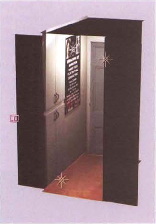
To light the geometry, create two point lights. To do so, choose Layer → New → Light. In the Light Settings dialog box, change the Light Type menu to Point and click OK. Position Light 1 near the ceiling and the door (see Figure 11.28). Position Light 2 near the floor and foreground walls. Set the Intensity value of Light 2 to 150%. You can access the Light Options section for each light in the layer outline. Adjust the Material Options values for each 3D layer so that the lighting feels consistent. For example, set the
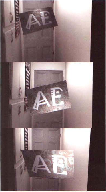
hall_door.tgalayer's Diffuse property to 50% and Specular property to 0%. This prevents a hot spot from forming on the door and making it inappropriately bright compared to the rest of the hallway.To test the depth of the scene, animate Camera 1 moving slowing across the hall. Play back the timeline to gauge the amount of parallax shift that's created. Create a new 3D layer and animate it moving through the hallway. For example, in Figure 11.29, an image with the word AE is converted to a 3D layer. Create a test render through the Render Queue. To render with motion blur, toggle on the Motion Blur layer switch for each of the 3D layers in the layer outline. If you'd like to see the blur in the viewer, toggle on the Motion Blur composition switch. The tutorial is complete. A sample After Effects project is included as
ae11.aepin the Tutorials folder on the DVD.
Nuke allows you to import geometry and project textures within the 3D environment.
Create a new script. Choose Edit → Project Settings. In the Project Settings properties panel, change Frame Range to 1, 24. Change the Full Size Format value to 1K_Super_35 (Full App). In the Node Graph, RMB+click and choose Image → Read. Browse for
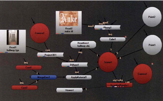
hallway.tgain the Footage folder in the DVD. Connect a viewer to the Read1 node.hallway.tgafeatures a hall and door. The goal of this tutorial will be to create a sense of 3D by projecting the image onto imported geometry.With no nodes selected, RMB+click and choose 3D → Geometry → ReadGeo. With the ReadGeo1 node selected, RMB+click and choose 3D → Scene. With no nodes selected, chose 3D → Camera. With no nodes selected, choose 3D → ScanlineRender. Connect the Obj/Scn input of the ScanlineRender1 node to the Scene1 node. Connect the Cam input of the ScanlineRender1 node to the Camera1 node. Connect the ReadGeo1 node to the Scene node. Connect a viewer to the ScanlineRender1 node. Use Figure 11.30 as a reference.
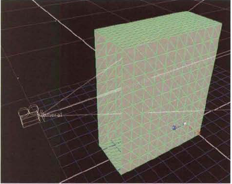
Open the ReadGeo1 node's properties panel. Browse for
hallway.fbxin the Footage folder on the DVD. At this stage, nothing is visible in the viewer. Change the View Selection menu, at the top right of the Viewer pane, to 3D. The imported geometry is visible, but it is so large that it extends past the edge of the frame. The geometry is a simplified model of the hallway. However, because it was accurately modeled on inch units in Maya, it becomes extremely large when imported into a 3D environment that utilizes generic units. In the ReadGeo1 node's properties panel, change the Uniform Scale slider to 0.032. A uniform scale of 0.032 makes the geometry approximately 8 units tall, which is equivalent to 8 feet, or 96 inches. Use the camera keys (Alt+LMB, Alt+MMB, and Alt+RMB) in the viewer to frame the camera icon and imported geometry. The Camera1 icon remains inside the geometry. Select the Camera1 icon and translate it to 0, 4, 12 (see Figure 11.31).With no nodes selected, RMB+click and choose 3D → Shader → Project3D. Connect the output of Read1 to the unlabeled input of Project3D1. With no nodes selected, RMB+click and choose 3D → Shader → Diffuse. Connect the output of Project3D1 to the input of Diffuse1. Connect the Img input of ReadGeo1 to Diffuse1. Select the Camera1 node and choose Edit → Duplicate. Connect the output of the new Camera2 node to the Cam input of Project3D1. Use Figure 11.30 earlier in this section as a reference. This projects the hallway image onto the hallway geometry from the point of view of Camera2.
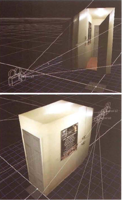
Figure 11.32. (Top) The initial projection. The Camera1 and Camera2 icons overlap. (Bottom) Camera2's Focal Length, Translate, and Rotate parameters are adjusted, creating better projection coverage. Note how the door is aligned with the back plane of the geometry and the ceiling is aligned with the top plane.
Initially, the projection is too small (see Figure 11.32). Select the Camera2 icon and interactively translate and rotate it until the projection covers the entire geometry. The goal is to align the edges of the geometry with the perspective lines of the image. For example, the ceiling-to-wall intersections of the image should line up with the side-to-top edge of the geometry. A translation of 0.4, 4.2, 16 and a rotation of −1.5, 3, 0 work well. One important consideration is the focal length of the projecting camera. Ideally, the focal length of Camera2 should match the focal length of the real-world camera used to capture the image. However, since
hallway.tgawas doctored in Photoshop, an exact match is not possible. Nevertheless, if Camera2's Focal Length property is set the 45, the match becomes more accurate. An additional trick for aligning the projection is to examine the hallway geometry from other angles in the 3D view. In such a way, you can check to see if the image walls are aligned with the geometry planes (see Figure 11.32). For example, the door should appear on the back plane of the geometry without overlapping the side planes. In addition, the floor and ceiling shouldn't creep onto the back or side planes.You can fine-tune the projection by adjusting Camera2's Window Scale parameter (in the Projection tab). The parameter allows you to scale the projection without manipulating the camera's transforms. In addition, you can stretch the projection in the X or Y direction. With this setup, a Window Scale value of 1.1, 1.35 provides a more exact match. You can also adjust the Translate, Rotate, and Scale properties of the ReadGeo1 node if necessary. Since the geometry is too short in the Z direction, which causes the cabinets to be cut off, set the ReadGeo node's Scale Z value to 1.25.
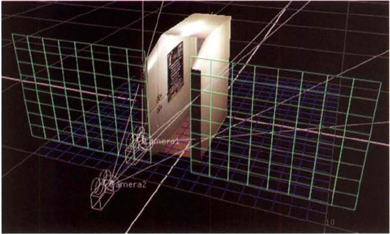
Return to the 2D view. The projection is working at this stage. However, the geometry doesn't cover the left and right foreground walls. To create walls, add two cards. With no nodes selected, RMB+click and choose 3D → Geometry → Card two times. With no nodes selected, RMB+click and choose 3D → Modify → MergeGeo. Connect the output of Card1 and Card2 to MergeGeo1. Use Figure 11.30 earlier in this section as a reference. With MergeGeo1 selected, RMB+click and choose 3D → Shader → ApplyMaterial. Connect the output of ApplyMaterial1 to Scene1. Connect the Mat input of ApplyMaterial1 to the output of Diffuse1. These connections allow the Camera2 projection to texture both cards. Open the Card1 and Card2 nodes' properties panels. Change the Uniform Scale setting for each one to 10. Translate Card1 in the viewer so that it forms the left foreground wall (see Figure 11.33). Translate Card2 in the viewer so that it forms the right foreground wall.
Create two point lights (3D → Lights → Point). Connect both Point nodes to Scene1. Position Point1 in the viewer so that it sits near the ceiling of the hall. Position Point2 near the floor between Card1 and Card2 (see Figure 11.34). Set the Intensity slider for Point2 to 0.1. Although the hallway geometry does not require lighting (the Project3D1 node brings in the projected texture at 100% intensity), any additional geometry must be lit to be seen.
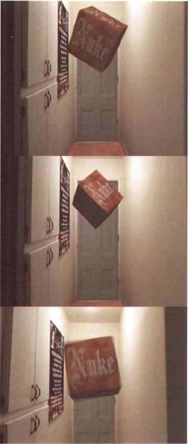
To test the depth of the 3D environment, animate Camera1 moving slowly across the hall. Play back the timeline to gauge the amount of parallax shift that's created. Create a new piece of geometry and animate it moving through the hallway. For example, in Figure 11.35, a Cube node is added. The cube is textured with a Phong shader and a Read node with a texture bitmap. Animate the geometry moving toward the camera to increase the sense of depth in the scene. Test the animation by rendering with Render → Flipbook Selected. To increase the render quality and activate motion blur, increase the Samples slider in the MultiSample tab of the ScanlineRender node's properties panel. The tutorial is complete. A sample Nuke script is included as
nuke11.nkin the Tutorials folder on the DVD.
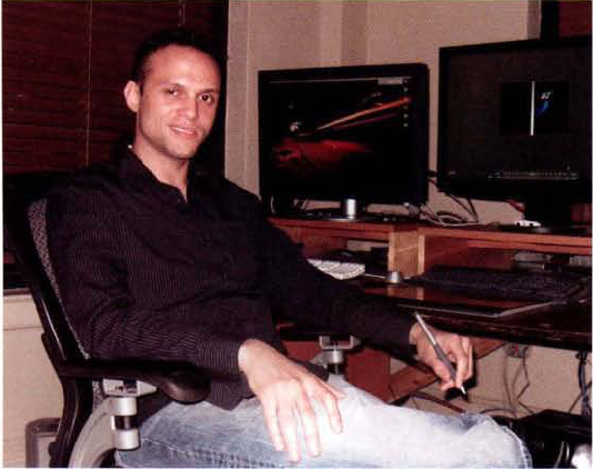
In 2002, David Schnee graduated from the Academy of Art University in San Francisco. While at school, he specialized in compositing and visual effects, working in Combustion, After Effects, and Flint. Four months after graduation, he was hired by Tippett to work on Starship Troopers 2. Thrown into a production environment, he quickly learned to use Shake. His feature credits now include Constantine, Cloverfield, The Spiderwick Chronicles, Drag Me to Hell, and X-Men Origins: Wolverine.
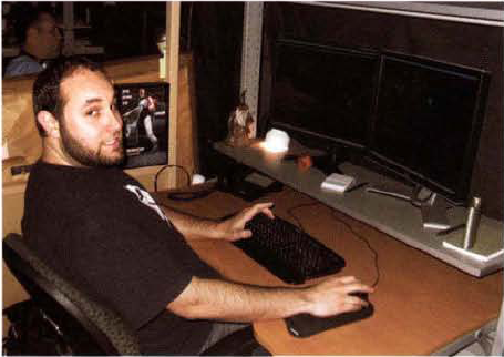
David Schnee at a workstation. Note that the compositing program, in this case Shake, is spread over two monitors.
Phil Tippett founded Tippett Studio in 1984. The venture literally started in Phil's garage, where he created stop-motion animation. It has since grown to a world-class facility with five buildings and over 200 employees in Berkeley, California. Over the past two decades, Tippett has created visual effects for over 60 feature films and has earned multiple Emmys, CLIOs, and Academy Awards. Feature credits include Robocop, Ghost Busters, Jurassic Park, and Hellboy.
(Tippett uses Shake and, secondarily, After Effects. At present, the studio keeps 25 compositors on staff, but the total expands and contracts depending on the projects on hand. Compositors are separated into their own compositing department.)
LL: What has been the biggest change to compositing in the last 10 years?
DS: [T]he biggest change includes a couple of things—one is [the] blurry line between 2D and 3D in the composite. [The second is] the ever-increasing...responsibility of the compositing artist. This includes becoming more responsible earlier in the pipeline [by] performing re-times (color grades) on plates, working with every breakout (render) pass imaginable, [and the need] to re-light and fix [problems created by] departments up stream.... [For] artists working with higher-end software such as Nuke, [this includes] using projection mapping techniques [with imported] geometry. [I]n some cases, [this entails] lighting environments with HDRI images or building a new camera move from the existing plate with projections.... [The] ability to...build an entire environment...in the composite is most definitely a big change for us. At Tippett, we perform these same techniques, but it's handled in our matte painting department. It's only a matter of time before we will be performing these same tasks in our [compositing] department.
LL: What is the most exciting change that you see on the horizon?
DS: 3-D. If the stereoscopic thing takes off (we'll find out in the next year or so), we'll need to think and composite in...new ways, accounting for each eye and manipulating layers of each eye to get the most from the 3-D and convergence points. We'll also need better asset management due to the doubling of the amount of rendering and layers to account for both left and right eye.
LL: Is there any leap in technology that you would like to see happen?
DS: I would love to be able to work more in "real time." [T]oo much time is spent waiting on GUI updates, filtering, and processing math operations. I'm not sure what the answer is, but it would be great to work in an environment where you can build and test operations and see the results much faster.... [W]orking at 2K in real time could happen, but as projects demand more detail and better quality, working at 4K will [become] the norm, and doubling up on just about everything in the pipeline will eat away at that real-time workflow we might get [if we just worked with] 2K.
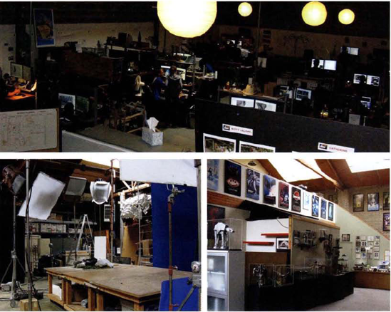
(Top) One of several rooms dedicated to animators at Tippett Studio (Bottom Left) A sound stage used to shoot miniatures and other live-action elements (Bottom Right) The main lobby, which includes numerous models from feature film work, including The Empire Strikes Back and Starship Troopers.
Aaron Vasquez graduated from the School of Visual Arts in New York City, where he specialized in CG modeling and texturing. He began his career with SMA Realtime, where he was able to train himself on an Inferno station. He made the transition to visual effects work when he later moved to Sideshow Creative. In 2005, he joined Click 3X as a Flame artist. In the past four years, he's provided effects for a variety of brands, including Pantene, Sharp, Time Warner, and Samsung.
Aaron Vasquez at his Flame station.
Click 3X was founded in 1993, making it an early adopter of digital technology. The studio offers branding, image design, motion graphics, and visual effects services for commercials, music videos, and feature film as well as the Web and mobile media. The studio's recent client roster includes MTV, Burger King, and E*Trade.
(Click 3X uses Flame, Smoke, After Effects, Shake, and Nuke. The studio has five compositors in-house.)
LL: Do you visit the set when there is a live-action shoot?
AV: Yes. I'll go sometimes and serve as visual effects supervisor. A lot of times I'll take my laptop with me—get a video tap straight into my laptop and I'll do on-set comps for the clients, who are usually nervous about what's going to happen.... It's a great tool to ease their fears....
LL: What do you use on location to create the composites?
AV: I'll use After Effects to do the comps on the fly.
LL: Since you're on set, what data is important to bring back with you?
AV: If it's motion control, any of the motion control data—the ASCII files (text data files) that they provide...any measurements—that's always important.... [W]hat I'm finding now too is that the CG guys will ask me to [take] 360° panoramas for them so that they can re-create the lighting with HDRIs. I'll bring a lighting ball (a white ball used to capture the on-set light quality) with me...and a mirror ball.... We have a Nikon D80 we use for the photos.
LL: How common is it to work with 2.5D?
AV: It's very common. Almost every other job is multiplaning these days. A lot of the work I've been doing lately is taking [the 2.5D] to the next level—instead of just multiplaning on cards, I'll project [images] onto CG geometry in Flame.... One of my strengths originally was as a [CG] modeler, so I'll model objects in Lightwave...and bring it in as an OBJ or Max 3DS files. I usually take care of the texturing in Flame. It's instantaneous. [Flame] has built-in geometry also....
