
"Know the math behind what you are doing. A over B-What does that mean? You have to know the procedure-you have to know why."

Filters, in the form of effects and nodes, are an integral part of compositing. Many common filters, such as blur and sharpen, are based on a convolution kernel. Such kernels, which are detailed in this chapter, are equally capable of creating stylized effects, such as emboss and edge enhance. After Effects and Nuke provide a long list of convolution-style filters. Nuke offers Convolve and Matrix nodes that allow you to design your own custom convolutions. Hence, it's important to understand how kernel values affect the output. A number of sample kernels are included in this chapter. In addition, you will have the chance to update the work started with the Chapter 5 tutorial. In addition, you'll build a custom filter using existing effects and nodes.

As discussed in Chapter 5, using matrices is a necessary step when applying transformations to a layer or node output. Not only is position, rotation, skew, and scale information stored in a transformation matrix, but pixel averaging, which is required to prevent aliasing problems, is undertaken by convolution matrices. You can also apply convolution matrices to create stylistic effects. In fact, such matrices serve as the basis of many popular compositing filters that are discussed in this chapter.
Blurs are one of the most common filters applied in compositing. They may take the form of a box filter, where all the kernel elements are identical and a divisor is employed. They may also take the form of a tent filter, where the weighting of the kernel tapers towards the edges. An example tent filter kernel follows:
1 2 1
1/16 2 4 2
     1 2 1
This kernel does not include brackets, although the matrix structure is implied. In addition, the kernel includes a divisor in the form of 1/16. A divisor forces the end sum of the kernel multiplication to be multiplied by its fractional value. The use of a divisor ensures that the resulting image retains the same tonal range as the original. In this case, 16 is derived from the sum of all the matrix elements. You can express the same kernel as follows:
1/16 2/16 1/16
2/16 4/16 2/16
1/16 2/16 1/16
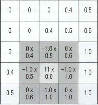
If a convolution kernel does not indicate a divisor, it's assumed that the divisor is 1.0 / 1.0, or 1.0. If the divisor is a value other than 1.0, averaging occurs across all pixel values found below the kernel. For example, in Table 6.1, a 5×5 input image is represented by an input matrix. Each input matrix cell carries a pixel value. The filter kernel is represented by the dark gray cells. In this position, the kernel determines the output value of the pixel colored light gray, which lies under the kernel's central element. The convolution math for this kernel position can be written in the following manner:
x = ((1.0 × 1.0) + (2 × 1.0) + (1.0 × 0.5) + (2 × 1.0) + (4 × 1.0) +
(2 × 0.5) + (1.0 × 1.0) + (2 × 1.0) + (1.0 × 0.5)) / 16

The output value x for the targeted pixel is thus 0.875. The application of this particular filter kernel creates the output image illustrated by Figure 6.1. (For more information on box filters, tent filters, and kernel convolution, see Chapter 5.)

Figure 6.1. (Left) 5×5 pixel image that matches the input matrix illustrated by Table 6.1 (Right) Same image after the convolution of the example blur kernel. A sample Nuke script is included as 5x5blur.nk in the Tutorials folder on the DVD.
Blur kernels are not limited to a specific kernel size. For example, Gaussian blurs are often expressed as 5×5 matrices with whole values:
1 4 6 4 1
      4 16 24 16 4
1/256 6 24 36 24 6
      4 16 24 16 4
      1 4  6  4  1
Gaussian blurs form a bell-shaped function curve and are thus similar to the cubic filters discussed in Chapter 5. The blurs take their name from Johann Carl Friedrich Gauss (1777–1855), a mathematician who developed theories on surface curvature.
You can create a directional blur by aligning non-0 elements so that they form a line in a particular direction. For example, the following kernel creates a blur that runs from the bottom left of frame to the right of frame:
0   0   0   0
1/4 0   0   0.3 1
    0   0.6 0.7 0
    1   0.4 0   0
Any pixel that falls under a 0 element is ignored by the pixel averaging process (see Figure 6.2). If the input image has a large resolution, the kernel matrix must have a large dimension for it to have a significant impact. Otherwise, the resulting blur will be subtle.

Sharpening filters employ negative values in their kernels. For example, a generic sharpen kernel can be written in the following manner:
0 −1   0
−1  11 −1
 0 −1   0
As is the case with many sharpening filters, the divisor is 1.0. The negative values, on the other hand, are able to increase contrast within the image by exaggerating the differences between neighboring pixels. For example, in Table 6.2, a 5×5 input image of a soft, diagonal edge is represented by an input matrix. The central element of the matrix kernel is set to 11. The higher the central element, the more extreme the sharpening and the brighter the resulting image.
In Table 6.2, the filter kernel is represented by the dark gray cells. In this position, the kernel determines the output value of the pixel colored light gray. The output value for the targeted pixel is thus 3.6. The application of this particular filter kernel creates the output image illustrated by Figure 6.3.
Because four of the input pixels along the edge of the kernel are multiplied by −1, their values are subtracted from the target pixel value. If the central kernel element does not have a high enough value, either little sharpening occurs or the output image becomes pure black. For example, if the central element is changed from 11 to 2, the output value for the target pixel becomes −1.8 through the following math:
x = 0 − 0.5 + 0 − 0.5 + (2 × 0.6) − 1.0 + 0 − 1.0 + 0
Values below 0 or above 1.0 are either clipped or normalized by the program employing the filter. If they are normalized, the values are remapped to the 0 to 1.0 range.

Figure 6.3. (Left) 5×5 pixel image that matches the input matrix illustrated by Table 6.2 (Right) Same image after the convolution of the example sharpen kernel. A sample Nuke script is included as 5x5sharpen.nk in the Tutorials folder on the DVD.
Unsharp mask filters apply their own form of sharpening. Although there are different varieties of unsharp masks, they generally work in the following manner:
An edge detection filter is applied to an input (see the next section).
The result is inverted, blurred, and darkened.
The darkened version is subtracted from the unaffected input.
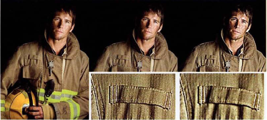
When a strong sharpen filter is compared to the strong unsharp mask filter, differences are detectable. For example, in Figure 6.4, the sharpened image contains numerous fine white lines in the cloth of the jacket. The same lines are more difficult to see in the unsharp mask version. However, the unsharp version creates a greater degree of contrast throughout the image.
For examples of custom unsharp filters, see the AE and Nuke tutorials at the end of this chapter.
Several stylistic filters employ negative element values in a limited fashion. These include edge enhance, edge detection, and emboss.
A simple edge enhance kernel can be written like this:
0  0 0
0 −8 0
0  8 0
With this kernel, any high-contrast edge whose bright side faces the bottom of the frame is highlighted (see Figure 6.5). The remainder of the image is set to black. The variations in line color result from the application of the kernel over pixels with unequal RGB values. To highlight a different set of edges, move the 8 to a different edge element of the matrix.
Edge detection kernels vary from edge enhance kernels in that they detect edges that run in all directions (see Figure 6.6). Common edge enhance kernels are based upon a Laplace transform, which is an integral transform named after mathematician Pierre-Simon Laplace (1749-1827). Essentially, an integral transform maps an equation from one domain to another in a bid to simplify its complexity.
A Laplacian filter may be expressed as a 3×3 kernel:
−1 −1 −1
−1  8 −1
−1 −1 −1
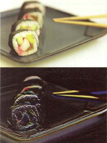
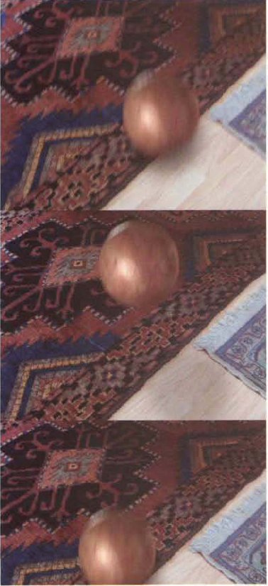
Figure 6.5. (Top) Input image (Bottom) Result of edge enhance kernel (Photo © 2009 by Jupiterimages)
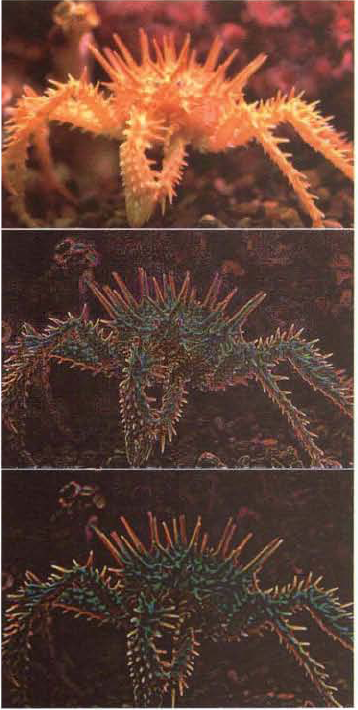
Figure 6.6. (Top) Input image (Center) Edge detection result (Bottom) Edge detection with initial blur (Photo © 2009 by Jupiterimages)
In the realm of digital image processing and compositing, Laplacian filters often refer to a two-step operation which applies a Gaussian blur kernel first and an edge detection kernel second. Blurring the input matrix first prevents the edge detection kernel from creating fine noise (see Figure 6.6). It's also possible to convolve the Gaussian kernel and the Laplacian filter first, and then convolve the resulting hybrid kernel with the input matrix. The hybrid kernel is referred to as Laplacian of Gaussian.
Sobel filters only test for high-contrast areas that run in either the X direction or the Y direction. To test for both directions, two kernels are required, as in this example:
1  2  1  −1 0 1
 0  0  0  −2 0 2
−1 −2 −1  −1 0 1
Because Sobel filters test horizontally and vertically, they generally do not produce edges as clean as Laplacian filters. Sobel filters, like many edge detection filters, suffer from noise and benefit from an initial blur.
Emboss filters lighten pixels in a particular direction while darkening neighboring pixels in the opposite direction. An example of an emboss kernel follows:
−10 −5  1
1/3 −5   10 5
     1   5  1
With this kernel, high-contrast edges that favor the lower-right corner of the frame are made brighter (see Figure 6.7). High-contrast edges that favor the upper-left corner of the frame are made darker. When you place a brighter or darker edge along features, you gain the illusion of bumpiness. Since a divisor is used, the original image remains visible within the embossing. Much like Laplacian filters, emboss filters benefit from the initial application of a blur filter.
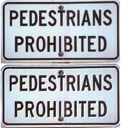
Figure 6.7. (Top) Input image (Right) Result of blur kernel and emboss kernel (Photo © 2009 by Jupiterimages)
After Effects and Nuke provide numerous convolution-based filters. In addition, Nuke offers a Convolve and a Matrix node with which you can write your own custom convolutions. These nodes, along with the most useful filters, are discussed later in this chapter.
After Effects and Nuke provide numerous effects and nodes with which to apply convolution filters. The filter types include blurs, sharpens, and stylistic effects.
Filters are referred to as effects in After Effects. You can find convolution-based effects under the Blur & Sharpen and Stylize menus. In addition, the program provides a layer-based motion blur function.
After Effects can create motion blur for any layer that transforms over time. The blur length is determined by the distance the layer moves over the duration of one frame. In essence, the blur path lies along a vector that's drawn from each pixel start position to each pixel end position.
To activate motion blur, toggle on the Motion Blur layer switch for a specific layer within the Timeline panel (see Figure 6.8). By default, the blur will not be visible in a viewer. However, if you toggle on the Motion Blur composition switch, the blur appears. Whether or not motion blur is rendered through the Render Queue is determined by the Motion Blur menu of the Render Settings dialog box. By default, the menu is set to On For Checked Layers (checking is the same as toggling on the Motion Blur layer switch). For more information on switches and the Render Queue, see Chapter 1. For an example of layer-based motion blur, see "AE Tutorial 5 Revisited: Creating a Shadow and a Camera Move" at the end of this chapter.

Figure 6.8. (Left) Motion Blur layer switch toggled on for one layer (Right) Motion Blur composition switch toggled on
You can adjust the length of a motion blur trail by changing the composition's Shutter Angle value. To do so, choose Composition → Composition Settings, switch to the Advanced tab of the Composition Settings dialog box, and change the Shutter Angle cell. Lower values shorten the blur trail and higher values lengthen the blur trail. Since the property emulates the spinning shutter disk of a motion picture camera, its measurement runs from 0 to 360°. The Shutter Phase property, which is found in the same tab, controls the time offset of the blur. Positive Shutter Phase values cause the blur to lag behind the moving element. Negative values cause the blur to precede the element. For realistic results, it's best to leave the Shutter Phase set to the equation Shutter Angle/−2.
After Effects provides several blur and sharpen effect variations. The most useful are discussed in the following sections. The effects are accessible through the Effect → Blur amp; Sharpen menu.
The Fast Blur effect is an approximation of the Gaussian Blur effect that is optimized for large, low-contrast areas. The Blurriness slider controls the size of the filter kernel and thus the intensity of the blur. You can choose to blur only in the vertical or horizontal direction by changing the Blur Dimensions menu to the direction of your choice. When selected, the Repeat Edge Pixels check box prevents the blur from introducing a black line around the edge of the layer. Instead of allowing the kernel to use 0 as a value when it overhangs the edge of input image matrix, the Repeat Edge Pixels check box forces the kernel to use the nearest valid input pixel value.
In comparison, the Gaussian Blur effect uses a kernel matrix that is similar to the Gaussian filter described in the section "Blurring Kernels" earlier in this chapter. Due to the filter's bell-shaped function curve, the blur is less likely to destroy edge quality. Unfortunately, the effect does not possess a Repeat Edge Pixels check box, which leads to the blackening of the layer edge. Aside from the edge quality, Fast Blur and Gaussian Blur effects appear almost identical when the layer's Quality switch is set to Best. When the layer's Quality switch is set to Draft, however, the Gaussian Blur effect remains superior to the Fast Blur effect, which becomes pixilated.
Additionally, the Box Blur and Channel Blur effects base their functionality on the Fast Blur effect. Box Blur adds an Iterations slider that controls the number of sequential blurs that are added and averaged together. If Iterations is set to 1, the result is pixilated but the speed is increased. A value of 3 produces a result similar to Fast Blur. Higher values improve the smoothness of the blur. The Channel Blur effect allows you to set the Blurriness value for the red, green, blue, and alpha channels separately. This may be useful for suppressing noise. For example, you can apply the Channel Blur effect to the blue channel of video footage while leaving the remaining channels unaffected. Thus the noise strength is reduced without drastically affecting the sharpness of the layer.
The Directional Blur effect adds a linear blur as if the camera were moving in a particular direction. With the Direction control, you can choose an angle between 0° and 359°. The length of the blur trail is set by the Blur Length slider.
In contrast, the Radial Blur effect creates its namesake (as if the camera were rotated around an axis running through the lens). The Amount slider controls the blur strength. The center of the blur is determined by the Center X and Y cells. You can interactively choose the center by LMB+dragging the small bull's-eye handle in the viewer of a Composition panel. You can convert the Radial Blur effect to a zoom-style blur by changing the Type menu to Zoom. The blur is thereby streaked from the center to the four edges of the image. The smoothness of the resulting blur is set by the Antialiasing menu, which has a Low and High quality setting.
The Compound Blur effect bases its blur on a control layer, defined by its Blur Layer menu. High luminance values within the control layer impose a greater degree of blur onto corresponding pixels within the layer to which the effect is applied. For example, in Figure 6.9, a layer with a white star serves as the control layer. The resulting blur is thus contained within the star shape. The maximum size of the kernel and strength of the blur is established by the Maximum Blur slider. By selecting the Invert Blur check box, you can make the blur appear where the control layer has low luminance values.
The Lens Blur effect takes the control layer technique further by offering additional properties. The control layer is selected through the Depth Map Layer menu. (Despite its name, the Depth Map Layer property can use a Z-buffer channel only if it is converted to RGB first.) The Depth Map Channel menu determines what channel information is used for the blur (luminance, R, G, B, or A). Blur Focal Distance determines which pixel values within the control layer are considered to be at the center of the virtual depth of field. The slider operates on an 8-bit scale, running from 0 to 255. If the slider is set to 150, for example, the region is centered at pixels with values of 150. Neighboring pixels with values ranging from roughly 100 to 150 and 150 to 200 are considered "in focus" with the sharpness tapering off toward lower and higher values. As an example of the Lens Blur effect, in Figure 6.10 a boardwalk is given an artificially narrow depth of field. The control layer is a mask that outlines the foreground buildings. In this case, the Blur Focal Distance is set to 98.
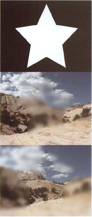
Figure 6.9. (Top) A control layer with a white star (Center) Resulting blur created with the Compound Blur effect (Bottom) Same effect with the Invert Blur check box selected. A sample After Effects project is included as compound_blur.aep in the Tutorials folder on the DVD.
Lens Blur provides three properties to control the bokeh shape of the virtual lens: Iris Shape, Iris Rotation, and Iris Blade Curvature. Bokeh describes the appearance of a point of light when it is out of focus. (For bokeh examples, see the section "Custom Convolutions" later in this chapter.) You can set the Iris Shape menu to several primitive shapes, including Triangle, Square, and Hexagon. The orientation of the resulting shape is controlled by Iris Rotation. To smooth off the corners of the shape, increase the Iris Blade Curvature value.
The Iris Radius slider sets the size of the filter kernel and the strength of the blur. Since the blurring operation removes noise and grain in the blurred region, Noise Amount and Noise Distribution add noise back to the image. Note that these two properties add noise to the blurred region only. In the same fashion, you can increase the intensity of bright areas within the blurred region by adjusting the Specular Brightness and Specular Threshold sliders. For a pixel to be brightened by Specular Brightness, it must have a value higher than the Specular Threshold value.

Figure 6.10. (Top Left) Layer without blur (Top Right) Black-and-white control layer (Bottom Left) Resulting Lens Blur. The foreground and background are blurred, while the mid-ground retains a narrow depth of field. Note that the blur averaging brightens the layer. (Bottom Right) Lens Blur settings. A sample After Effects project is included as lens_blur.aep in the Tutorials folder on the DVD.
The Unsharp Mask effect applies a standard unsharp filter as described in the section "Unsharpening" earlier in this chapter. The Radius slider determines the size of the kernel and the strength of the blur applied to a darkened version of the input. The Threshold slider establishes the contrast threshold. Adjacent pixels, whose contrast value is less than or equal to the Threshold value, are left with their input values intact. Adjacent pixels with a contrast value greater than the Threshold value receive additional contrast through the subtraction of a darker, blurred version of the input.
The Sharpen effect adds its namesake and uses a filter kernel similar to those demonstrated in the section "Sharpening Kernels" earlier in this chapter.
After Effects includes several stylistic filters that utilize convolution techniques. For example, the Smart Blur effect, found in the Blur & Sharpen menu, employs multiple convolution kernels. If the effect's Mode menu is set to Edge Only, the effect becomes an edge detection filter. If Mode is set to Normal, the effect operates as a median filter; this results in a painterly effect where small detail is lost and the color palette is reduced. As such, the effect determines the value range that exists within a group of neighboring pixels, selects the middle value, and assigns that value as the output for the targeted pixel. For example, in Figure 6.11, footage is given a painterly effect. In this case, the Radius slider is set to 50 and the Threshold slider is set to 100. Although a median filter employs a convolution, it also requires an algorithm with the ability to sort values. If Mode is set to Overlay Edge, an Edge Only version is added to the Normal version.
With the Smart Blur effect, the Threshold slider sets the contrast threshold for the filter. If the Threshold value is low, medium-contrast edges are isolated. If the Threshold value is high, a smaller number of high-contrast edges are isolated. The Radius slider, on the other hand, determines the size of the filter kernel. Large values lead to a large kernel, which in turn averages a greater number of pixels. If Mode is set to Edge Only, raising the Threshold reduces the number of isolated edges. If Mode is set to Normal, raising the Threshold reduces the complexity of the image, whereby larger and larger regions are assigned a single value.
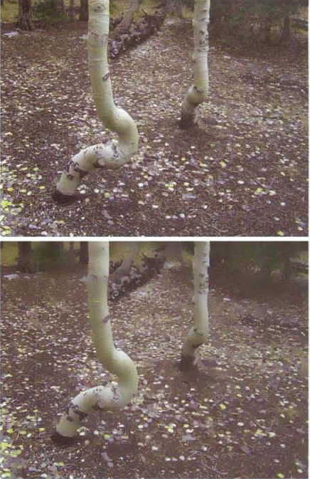
Figure 6.11. (Top) Layer with no blur (Bottom) Result of the Smart Blur effect with Mode set to Normal. A sample After Effects project is included as smart_blur.ae in the Tutorials folder on the DVD.
Emboss and Find Edges, found in the Stylize menu, create their namesake effects. For more information on these filters, see the section "Stylistic Filter Kernels" earlier in this chapter.
Nuke groups its filter nodes under a single Filter menu. These include nodes designed for custom convolutions, blurring and sharpening nodes, and stylistic effects nodes. In addition, Nuke provides node-based motion blur.
The Transform node includes a built-in method for motion blurring the node's output. To activate the blur, raise the Motionblur parameter above 0 (see Figure 6.12). If the node's Translate, Scale, Rotate, or Skew parameter is animated over time, the motion blur appears in the viewer. The quality of the blur is determined by the Motionblur value. The higher the value, the more samples are taken across time and the more accurate the blur trail is. Values between 1 and 3 are generally suitable for creating high-quality results.
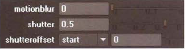
By default, the length of the motion blur is dependent on the distance each pixel travels over 1/2 frame. That is, the blur trail extends from the position of the element at the current frame to the position of the element 1/2 frame into the future. The 1/2 is derived from the default setting of the Shutter parameter, which is 0.5.
The motion blur length can be written as the formula frame to (frame + Shutter). To alter this formula, you can change the Shutteroffset parameter. The Shutteroffset menu is set to Start by default but has these additional options:
Centered If Shutter is set to 0.5, the Centered option goes back in time 1/4 frame and forward in time 1/4 frame to create the blur trail. The formula is (
frame - Shutter/2) to (frame + Shutter/2).End The End option uses the formula (
frame - Shutter) to frame.Custom The Custom option uses the formula (
frame + offset) to (frame + offset + Shutter). The offset is determined by the Shuttercustomoffset cell to the immediate right of the Shutteroffset menu.
For a demonstration of node-based motion blur, see "Nuke Tutorial 5 Revisited: Creating a Shadow and a Camera Move" at the end of the chapter.
Nuke offers the user a way to create a custom convolution kernel. This opens up almost endless possibilities when filters are applied. To create a custom kernel, follow these steps:
Select the node to which you want to apply the custom kernel. RMB+click and choose Filter → Matrix. In the Enter Desired Matrix Size dialog box, enter the matrix width and height. Although many standard filters use a matrix with an equal width and height, such as 3×3, you can create one with unequal dimensions, such as 5×4.
Connect the Matrix1 node to a viewer. Since the matrix is empty, the image is black. Open the Matrix1 node's properties panel. Enter a value into each matrix element cell. The values can be negative, positive, or 0 (see Figure 6.13).
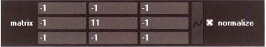
Figure 6.13. A 3×3 matrix provided by the Matrix node. The values entered into the matrix element cells create a sharpening effect.
For sample matrices, see the section "Filter Matrices" at the beginning of this chapter. Several re-creations of common filters have also been included in the Tutorials folder on the DVD:
sharpen.nk      Simple sharpen filter kernel
edge_enhance.nk Simple edge enhance kernel
emboss.nk       Simple emboss kernel
laplacian.nk    Laplacian filter re-created with a Blur and Matrix node
sobel.nk        Sobel filter using two Matrix nodes and a Blur node
In addition to the element cells, the Matrix node provides a Normalize check box. If this is selected, the resulting output values are divided by a divisor that is equal to the sum of the matrix elements. When selected, the Normalize check box guarantees that the output intensity is similar to the input intensity. Note that the Normalize check box will function only if the sum of all the matrix elements does not equal 0.
In addition to the Matrix node, Nuke supplies a Convolve node that can interpret a bitmap or other input as a kernel matrix. This is particularly useful when you are creating custom blurs that require a bokeh shape. To create such a blur, follow these steps:
Create a new script. In the Node Graph, RMB+click and choose Image → Read. In the Read1 node's properties panel, browse for an image or image sequence. (A sample image,
train.tif, is included in the Footage folder on the DVD.) With no nodes selected, RMB+click and choose Image → Read. In the Read2 node's properties panel, browse for a bitmap that will serves as the input kernel matrix. (A sample image,32bokeh.tif, is included in the Footage folder.)With no nodes selected, RMB+click and choose Filter → Convolve. Connect the output of the Read1 node to the input B of the Convolve1 node. Input B is reserved for the input that is to be affected by the convolution. Connect the output of Read2 to the input A of the Convolve1 node. Connect the output of Convolve1 to a viewer. The image is blurred. A sample script is saved as
convolve.nkin the Tutorials folder.
The convolution is inherently different from that of a standard Blur node. For example, in Figure 6.14, the two nodes are compared side by side.

Figure 6.14. (Left) Result of a Convolve node (Right) Result of a Blur node. The arrows point to bokehs created by the nodes. The Convolve node produces sharper bokeh shapes.
Real-world camera lenses create uniquely shaped bokehs when their depth of field is narrow or they are otherwise out of focus (see Figure 6.15). The most common bokeh is roughly circular, which corresponds to the shape of the camera's iris diaphragm, which is composed of overlapping triangular blades. Inexpensive cameras may have fewer blades and thus create bokehs that are more polygonal. It's also possible to create a custom bokeh shape by attaching a lens hood with the desired shape cut into it.
You can create stylized bokeh shapes by creating a bitmap with a particular pattern. The degree to which the input becomes out of focus is related to the size of the bokeh image (see Figure 6.16). That is, the image resolution determines the kernel matrix size. Hence, the 32bokeh.tif image, which is 32×32 pixels, is equivalent to a 32×32 kernel matrix. The larger the matrix is, the greater the degree of pixel averaging and the greater the degree of "out-of-focusness."
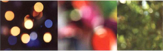
Figure 6.15. (Left) City lights at night from a distance (Center) Brightly colored objects that are close by, but are out of focus (Right) Out-of-focus trees located in the background (Photos © 2009 by Jupiterimages)
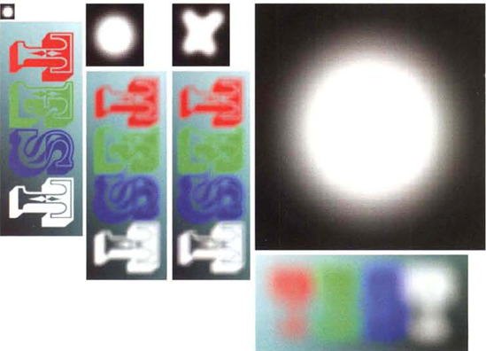
Figure 6.16. Custom blurs with corresponding bokeh bitmap files. The files are included as 8bokeh.tif, 32bokeh.tif, 128bokeh.tif, and xbokeh.tif in the Footage folder on the DVD.
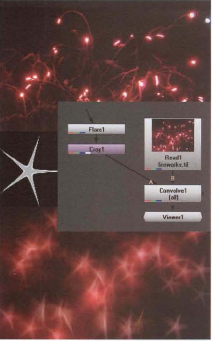
The Convolve node is able to use inputs other than bitmaps. For example, you can connect the output of a Flare node (Draw → Flare) to input A of a Convolve node. If the input resolution is too large, however, the convolution process may be significantly slowed. To make the process efficient, you can pass the input through a Crop node. For example, in Figure 6.17, a Flare node is adjusted to create a multipoint star. The Flare node is connected to a Crop node, which is set to a resolution of 100×100. (For more information on the Crop node, see Chapter 1.) The Flare node, along with similar draw nodes, is detailed in Chapter 10, "Warps, Optical Artifacts, Paint, and Text."
Nuke includes a number of nodes that blur and sharpen, all of which are found under the Filter menu.
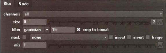
The Blur node offers a quick means to apply a standard blur filter (see Figure 6.18). The strength of the blur is set by the Size slider. The higher the Size value is, the larger the kernel matrix and the greater the degree of blurring. The smoothness of the blur is determined by the Quality cell (which is to the right of the Filter menu). Values below 15 downscale the input image; after the kernel is applied, the image is upscaled to its original size using a linear filter. Although the process speeds up the blur, it leads to pixelization. A value of 15, however, produces the most refined result. In addition, you can change the Filter menu to Box, Triangle, Quadratic, and Gaussian. The Box filter, which uses a function curve with no falloff, produces the weakest blur. The Triangle filter uses a tent-style function curve. The Quadratic filter, which uses a bell-shaped curve, produces the most aggressive blur. The Gaussian filter, which uses another variation of a bell-shaped curve, offers a good combination of quality and speed. For more information on blurring matrices, see the section "Filter Matrices" at the beginning of this chapter. For more information on filter function curves, see Chapter 5.
Despite its name, the Sharpen node applies an unsharp mask to an input (see Figure 6.19). (For more information, see the "Unsharping" section earlier in this chapter.) The Minimum and Maximum sliders set the size of the darkened regions along high-contrast edges. The Amount slider sets the degree to which the darkened regions are subtracted from the original. High Amount values create greater contrast within the image. Size controls the softness of the darkened regions.
The Soften node applies the same process as the Sharpen node. However, the result is added to the original input, creating a brighter, foggy result (see Figure 6.19).

The Defocus node is designed to create realistic depth-of-field blur that contains specific bokeh patterns. (For more information on bokeh, see the section "Custom Convolutions" earlier in this chapter.) Unlike the Convolve node, however, Defocus bases it bokeh shape on an Aspect Ratio slider. If Aspect Ratio is 1.0, small bright points produce circular spots. If Aspect Ratio is set at a value above 1.0, such as 1.33, 1.85, or 2.35, the circular highlight is stretched horizontally (see Figure 6.20).
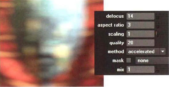
Figure 6.20. (Left) Input blurred with Defocus with an artificially high Aspect Ratio value of 3. Note the horizontal stretching of the bokeh shapes. (Right) Defocus settings. A sample Nuke script is included as defocus.nk in the Tutorials folder on the DVD.
The Defocus slider sets the degree of blurriness. The Scaling slider serves as a multiplier for the effect of the Defocus and Aspect Ratio parameters. In general, Scaling can be left at 1.0. Quality is true to its namesake with higher values producing better results. The Method menu provides Accelerated and Full Precision methods of interpolation. Accelerated is more efficient but may produce speckled noise in some situations. Full Precision guarantees maximum accuracy.
Nuke includes several specialized nodes that create unique blurs. These include EdgeBlur, DirBlur, Bilateral, and Laplacian.
The EdgeBlur node contains its blur to alpha edges. Size, Filter, and Quality parameters are identical to the Blur node. Edge Mult serves as a multiplier for the blur. Higher Edge Mult values increase the width of the blur; low values sharpen the blur. Tint, if set to a nonwhite value, tints the blurred area in the RGB channels. The ability to tint the edge offers a means to create a light wrap effect. (The Lightwrap node is discussed in Chapter 10.)
The DirBlur node applies a blur in one or more directions, thus emulating camera motion blur. The node offers three styles of blur through the BlurType menu: Zoom, Radial, and Linear (see Figure 6.21). Linear blur creates a blur trail in one direction (even if the input is static). Radial creates a circular blur as if the camera was spun on the axis that runs through its lens. Zoom creates a blur that runs from the center of frame to the four edges.
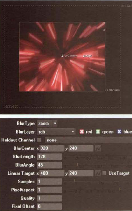
Figure 6.21. (Top) Zoom blur created by DirBlur node. The BlurCenter and Target handles are seen at the center of the viewer. Note that the blur extends the bounding box of the input. (Bottom) DirBlur settings. A sample Nuke script is included as dirblur.nk in the Tutorials folder on the DVD.
The center of a Zoom or Radial blur is determined by the BlurCenter parameter, which carries X and Y cells. You can interactively place the center by LMB+dragging the BlurCenter handle in a viewer. If BlurType is set to Linear, the direction of the blur trail is set by the BlurAngle slider. However, you can override BlurAngle by selecting the UseTarget check box. UseTarget activates the Linear Target parameter, which carries X and Y position cells. Linear Target forces the Linear blur trail to follow a vector drawn from the BlurCenter position to the Linear Target position. You can interactively change the Linear Target position by LMB+dragging the Target handle in a viewer. The BlurLength slider sets its namesake. The Samples slider determines how many offset iterations of the input are used to synthesis the blur. High values improve the smoothness of the blur but significantly slow the render. PixelAspect emulates different lens setups, whereby various values affect the shape of the blur trail. Values below 1.0 will warp a Zoom blur as if the virtual lens was wide-angle. Values below 1.0 will also vertically compress a Radial blur. The Quality parameter functions in the manner similar to the Quality parameter of the Blur node; however, a Quality setting of 1.0 creates a refined result, while high values lead to pixelization.
In contrast, the Bilateral node applies a selective blur to the input. Areas of low contrast receive a higher degree of blur, while areas of high contrast receive a lower degree of blur. This approach preserves edge sharpness (see Figure 6.22). The node's Size slider, in combination with the Positional Sigma slider, sets the intensity of the blur. High Positional Sigma values spread the blur into larger regions, obscuring fine detail. The Color Sigma slider determines the ultimate sharpness of high-contrast areas. Low values maintain edge sharpness. Although the Bilateral node produces a unique result, it operates more slowly than other blur nodes.
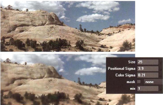
Figure 6.22. (Top Left) Detail of unaffected input (Bottom Left) Result of Bilateral node. Note how high-contrast crevices and treetops retain edge sharpness. (Bottom Right) Bilateral settings. A sample Nuke script is included as bilateral.nk in the Tutorials folder on the DVD
The Laplacian node, on the other hand, isolates edge areas by detecting rapid value change across neighboring pixels. Since the filter is prone to noise, however, blur is first applied to the input. The style of blur is controlled by the Filter menu, which is identical to the one provided by the Blur node. Each style affects the resulting thickness of the isolated edges to a different degree. The thickness is also influenced by the Size slider. For more information on Laplacian kernels, see the section "Stylistic Filter Kernels" near the beginning of the chapter.
The Emboss node creates a simple version of its namesake. The emboss kernel is also described in the section "Stylistic Filter Kernels." Additional stylistic Nuke nodes, which are not dependent on convolution techniques, are discussed in Chapter 10.
In this chapter, you'll have a chance to revisit tutorial 5, in which you'll fabricate a shadow, a camera move, and motion blur. In addition, two new tutorials will show you how to construct a custom unsharp mask using standard effects and nodes.
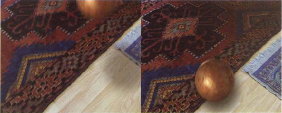
In Chapter 5, you gave life to a static render of a ball through keyframe animation. To make the animation more convincing, it's important to add a shadow. An animated camera and motion blur will take the illusion even further.
Reopen the completed After Effects project file for "AE Tutorial 5: Adding Dynamic Animation to a Static Layer." A finished version of Tutorial 5 is saved as
ae5.aepin the Chapter 5 Tutorials folder on the DVD. Play the animation. The ball is missing a shadow and thus a strong connection to the floor. Since the ball is a static frame and no shadow render is provided, you will need to construct your own shadow.Select the
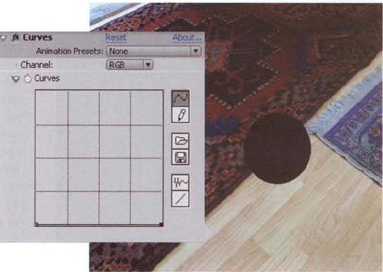
ball.tgalayer in the layer outline of the Timeline panel. Choose Edit → Duplicate. The layer is copied. Choose the lowerball.tgalayer (numbered 2 in the layer outline). This layer will become the shadow. For the moment, toggle off the Video switch beside the topball.tgalayer (numbered 1 in the layer outline). This temporarily hides the top layer. With the lowerball.tgalayer selected, choose Effect → Color Correction → Curves. In the Effect Controls tab, pull the top-right point of the curve line straight down so that the curve becomes flat (see Figure 6.23). Theball.tgalayer is changed to 0 black.With the lower
ball.tgalayer selected, choose Effect → Blur & Sharpen → Fast Blur. Change the Fast Blur effect's Blurriness slider to 100. Note that the amount of resulting blur is dependent on the resolution of the layer to which the blur is applied. Since this project is working at 2K, the Blurriness slider must be set fairly high to see a satisfactory result.Move the timeline to frame 6 (where the ball contacts the floor). Toggle on the Video switch beside the top
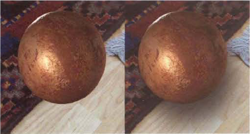
ball.tgalayer so that the layer is once again visible. The shadow will no longer be apparent because it is directly behind the top layer. To remedy this, select the lowerball.tgalayer, expand the Transform section, and toggle off the Stopwatch button beside the Position property. The keyframes for Position are removed. Interactively move the lowerball.tgalayer so that the shadow appears just below and to the right of the ball. Toggle on the Stopwatch button beside the Position property again to reactivate keyframing. A new keyframe is placed at frame 6. Move the timeline to each of the frames where the ball contacts the floor. Interactively move the lowerball.tgalayer so that the shadow appears just below the ball in each case. At this point, the shadow is inappropriately opaque and heavy. To fix this, change the lowerball.tgalayer's Opacity to 50% (see Figure 6.24).Move the timeline to each frame where the ball is at the top of a bounce. Interactively move the lower
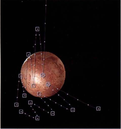
ball.tgalayer so that the shadow appears away from the ball and to the right. Assuming that the main light source is coming from frame left, the shadow should move toward frame right as the ball bounces up. However, as the bounce height decreases, so should the distance the shadow moves away from the ball. Once all the keyframes have been placed for the lowerball.tgalayer, select the new keyframes in the Timeline panel, RMB+click over a selected keyframe, and choose Keyframe Interpolation from the menu. In the Keyframe Interpolation dialog box, change Temporal Interpolation and Spatial Interpolation to Continuous Bezier. By changing both Interpolation types, you can interactively move the tangent handles via the Graph Editor and the overlay of the viewer. The layer should form a motion path overlay similar to Figure 6.25.Play back the timeline. At this point, the shadow opacity is consistent despite the movement of the ball. In a real-world situation, the shadow darkness would fluctuate as more or less ambient light is permitted to strike the shadow area. To emulate this effect, keyframe the Opacity property changing over time. For example, for the frames where the ball contacts the floor, keyframe Opacity at 50%. For the frames where the ball is at the peak of a bounce, keyframe Opacity at a value proportional to the ball's height off the floor. For example, if there are bounce peaks at frames 1, 11, 21, and 31, you can keyframe Opacity at 5%, 10%, 15%, and 20% respectively for those frames. Once the Opacity keyframes have been set, convert the new keyframes to temporal and spatial Continuous Bezier tangents (see step 5). To examine the result, open the Graph Editor (see Chapter 5 for additional details).
To add realism to the shadow, you can change the amount of blur applied to it over time. When the shadow is close to the ball, it should be sharper. When the shadow is farther from the ball, it should be softer. You can achieve this by keyframing the Blurriness property of the Fast Blur effect. For example, at frames 1, 11, 21, and 31, set the Blurriness value to 140, 130, 120, and 110 respectively. At frames 6, 16, 26, and 36, key the Blurriness value at 100.
At this stage, the ball bounce remains somewhat artificial due to a lack of motion blur. To create motion blur for the ball and shadow, select both
ball.tgalayers and toggle on their Motion Blur layer switches. The blur is not immediately visible but will be added to the final render. To see motion blur in the viewer, toggle on the Motion Blur composition switch at the top of the layer outline of the Timeline panel.Motion blur will also appear if any artificial camera move is created. To create such a move, you will need to nest two composites. Choose Composition → New Composition. In the New Composition dialog box, change Preset to NTSC D1 Square Pixel, Frame Rate to 30, Start Frame to 1, and Duration to 36.
LMB+drag Comp 1 from the Project panel and drop it into the Comp 2 tab of the Timeline panel. (For more information on nesting compositions, see Chapter 1.) Since Comp 2 is set to a 720×540 resolution, Comp 1 is oversized by default. Select the Comp 1 layer, expand its Transform section, and change the Scale property to 50%, 50%. This shrinks Comp 1 but makes it large enough to slide around the Comp 2 frame (see Figure 6.26).
Select Comp 1 and toggle on the Stopwatch button beside the Position property. Move to different frames and interactively position the Comp 1 layer so that it appears as if the camera is panning or tilting to follow the ball. Because the Stopwatch button is toggled on, keyframes are created each time there is a change in value. Only three of four keyframes are necessary to give the illusion of camera movement. Once you are satisfied with the keyframe placement, select the new keyframes and convert them to temporal and spatial Continuous Bezier tangents (see step 5).
Play back the timeline. To adjust the smoothness of the artificial camera move, manipulate the motion path overlay within the viewer. With the Comp 1 layer selected, set the viewer's Magnification Ratio Popup menu to 200% or 400% so that the motion path and keyframes are easily seen. Use the Hand tool to scroll the view to various parts of the motion path. To adjust a tangent, LMB+drag a tangent handle. To reposition a keyframe, and thus change the position of the Comp 1 layer for a particular frame, LMB+drag the keyframe box.
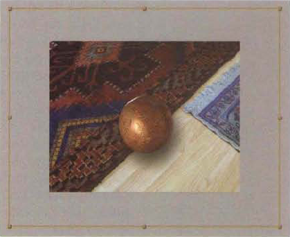
To add motion blur to the camera move, toggle on the Motion Blur switch for the Comp 1 layer. Render out a test movie using the Render Queue. When you play the rendered movie, you should see motion blur on the ball (see Figure 6.27). In addition, the entire frame will be blurred if the artificial camera makes a sudden move, such as a pan. If you see blur, the tutorial is complete. A sample After Effects project is included as
ae5_step2.aepin the Tutorials folder on the DVD.
In Chapter 5, you gave life to a static render of a ball through keyframe animation. To make the animation more convincing, it's important to add a shadow. An animated camera and motion blur will take the illusion even further.
Reopen the completed Nuke project file for "Nuke Tutorial 5: Adding Dynamic Animation to a Static Output." A finished version of Tutorial 5 is saved as
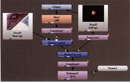
nuke5.aepin the Chapter 5 Tutorials folder on the DVD. Play the animation. The ball is missing a shadow and thus a strong connection to the floor. Since the ball is a static frame and no shadow render was provided, you will need to construct your own shadow.In the Node Graph, RMB+click, and choose Color → Clamp. Connect the output of the Read2 node to the input of the Clamp1 node. With the Clamp1 node selected, RMB+click and choose Transform → Transform. Disconnect the input A of the Merge1 node. Instead, connect input A to the output of the new Transform2 node. Refer to Figure 6.28 for node placement. Open the Clamp1 node's properties panel. Change the Channels menu to RGB and the Maximum slider to 0. This series of steps places a black version of the ball, which will become the shadow, on top of the floor.
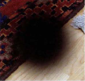
To soften the new shadow, select the Clamp1 node, RMB+click, and choose Filter → Blur. A Blur1 node is inserted between the Clamp1 and Transform2 nodes. Open the Blur1 node's properties panel and set the Size slider to 75. The shadow is softened (see Figure 6.29). To view the result, temporarily connect a viewer to the Merge1 node.
With no nodes selected, RMB+click and choose Merge → Merge. Connect the input A of the Merge2 node to the output of Transform1. Refer to Figure 6.28 for node placement. Connect the input B of Merge2 to the output of Merge1. Connect the output of Merge2 to a viewer. The original ball is placed back on top of the shadow and background.
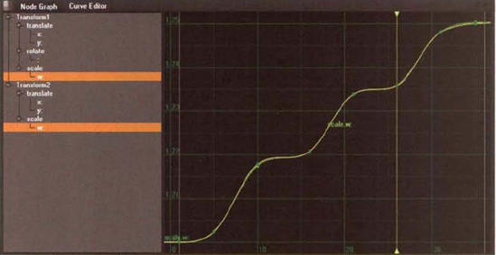
Open the Transform1 and Transform2 nodes' properties panels. Move the timeline to frame 5 (where the ball contacts the floor for the first time). Note the scale of the ball in the Transform1 node's properties panel. Set the Transform2 node's Scale value to match. Click the Animation button beside the Transform2 node's Scale slider and choose Set Key from the menu. Continue to every frame where Transfrom1 has a keyframe. Match Transform2's Scale value to Transform1. Any change to Transform2's Scale value will automatically create a new keyframe. To monitor the progress of the Transform2's Scale curve, open the Curve Editor. Match the shape of Transform2's Scale curve to Transform1's Scale curve by changing tangent types and manipulating tangent handles (see Figure 6.30). (For a review of the Curve Editor and tangent settings, see Chapter 5.)
Return the timeline to frame 5 (where the ball contacts the floor for the first time). Using the viewer transform handle, interactively move the shadow so that it's just below and to the right of the ball. In the Transform2 node's properties panel, click the Animation button beside the Translate parameter and choose Set Key. Move the timeline to each keyframe where the ball contacts the floor and interactively move the shadow to an appropriate location under the ball. New keyframes are automatically added to Transform2's Translate parameter.
Play back the timeline. (Make sure the viewer's Desired Playback Rate cell is set to 30 fps.) The shadow follows but stays directly below the ball. If the main light source is arriving from frame left, then a real-world shadow would change position with each bounce of the ball. To add appropriate shadow movement, move the timeline to frame 10 (the peak of the first bounce). Using the viewer transform handle, interactively move the shadow screen right. Move the timeline to each keyframe where the ball is at the peak of a bounce. Interactively move the shadow to an appropriate position. As the bounce height decreases, so should the distance the shadow moves away from the ball. The shadow should form a motion path overlay similar to Figure 6.31. To achieve the appropriately shaped curve, adjust the tangents for the Transform2 node's Translate X and Y curves in the Curve Editor.
Play back the timeline. At this point, the shadow is inappropriately opaque and heavy. To fix this, move the timeline to frame 5 (where the ball contacts the floor for the first time). Open the Merge1 node's properties panel. Change the Mix slider to 0.8. The shadow is more believable, yet the opacity is consistent despite the movement of the ball. In a real-world situation, shadow darkness fluctuates as more or less ambient light is permitted to strike the shadow area. To emulate this effect, keyframe the Mix value changing over time. First, move to each keyframe where the ball contacts the floor and force a keyframe for the Mix parameter. To force a keyframe, click the Animation button beside the Mix slider and choose Set Key. Next, move the timeline to the keyframes where the ball is at the peak of its bounce. Set the Mix parameter to a value proportional to the ball's height off the floor. For example, if there are bounce peaks at frames 1, 10, 21, and 31, you can keyframe the Mix value at 0.2, 0.3, 0.4, and 0.5 respectively.
To add realism to the shadow, you can change the amount of blur applied to it over time. When the shadow is close to the ball, it should be sharper. When the shadow is farther from the ball, it should be softer. You can achieve this by keyframing the Size parameter of the Blur1 node. For example, at frames 1, 10, 21, and 31, set the Size value to 115, 105, 95, and 85 respectively. At frames 5, 16, 26, and 35, key the Size value at 75.
At this stage, the ball bounce remains somewhat artificial due to a lack of motion blur. To create motion blur for the ball, open the Transform1 and Transform2 nodes' properties panels and change the Motionblur slider to 1.0. Motion blur is instantly added and appears in the viewer. Note that the blur significantly slows the speed with which the viewer renders each frame for playback.
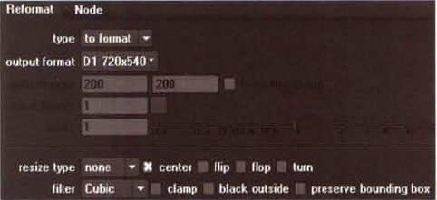
You can also apply motion blur to any artificial camera move. To create such a move, you will need to reformat the output. Select the Merge2 node, RMB+click, and choose Transform → Transform. Open the Transform3 node's properties panel and change the Scale slider to 0.5. This shrinks the image in anticipation of a smaller output format. With the Transform3 node selected, choose Transform → Reformat. This finishes the node network (see Figure 6.28 earlier in this section for reference). Open the Reformat1 node's properties panel. Change the Output Format menu to New. In the New Format dialog box, change File Size X to 720 and File Size Y to 540. Enter D1 as the Name and click the OK button. In the Reformat1 node's properties panel, change the Resize Type menu to None (see Figure 6.32). The composited image remains larger than the final output, which will allow you to move the image to create an artificial camera move.
Move the timeline to frame 1. Open the Transform3 node's properties panel. Click the Animation button beside the Translate parameter and choose Set Key. Change the timeline to different frames and interactively move Transform3 so that it appears as if the camera is panning or tilting to follow the ball. Only three of four keyframes are necessary to give the illusion of camera movement.
To add motion blur to the camera move, change the Motionblur parameter for Transform3 to 1.0. Play back the timeline until all the frames are rendered and the viewer is able to achieve 30 fps. When you stop the playback and scrub through the frames, you should see motion blur on the ball. In addition, the entire frame will be blurred if the artificial camera makes a sudden move, such as a pan. If the timeline is unable to play back the animation in real time, create a flipbook by selecting the Reformat1 node and choosing Render → Flipbook Selected. If you see blur, the tutorial is complete (see Figure 6.33). A sample Nuke script is included as
nuke5_step2.nkin the Tutorials folder on the DVD.

Although After Effects includes an Unsharp Mask effect, it's possible to build a custom unsharp mask by combing several other effects.
Create a new project. Choose Composition → New Composition. In the Composition Settings dialog box, set Preset to NTSC D1 Square Pixel and Duration to 1. Import
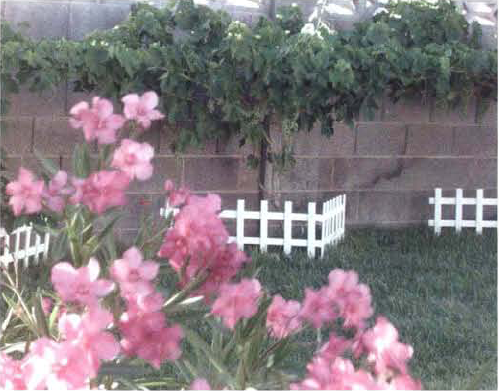
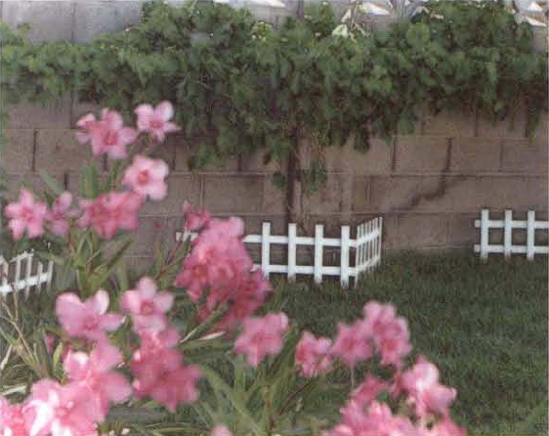
flowers.tiffrom the Footage folder on the DVD. LMB+dragflowers.tiffrom the Project panel to the layer outline of the Timeline panel. The image features a somewhat washed-out and soft view of a yard (see Figure 6.34).With the
flowers.tiflayer selected, choose Effect → Stylize → Find Edges. In the Effect Controls panel, select the Invert check box. The Find Edges effect isolates high-contrast edges through a Lapacian kernel. The Invert check box places bright edges over black. Choose Effect → Blur & Sharpen → Fast Blur. Set the Fast Blur effect's Blurriness to 10. Toggle on Repeat Edge Pixels to prevent a black edge. This represents the first step of an unsharp mask, which requires isolated edges to be blurred.Choose Composition → New Composition. In the Composition Settings dialog box, set Preset to NTSC D1 Square Pixel and Duration to 1. LMB+drag Comp 1 from the Project panel to the layer outline of the Comp 2 tab in the Timeline panel. LMB+drag
flowers.tiffrom the Project panel to the layer outline of the Comp 2 tab. The newflowers.tiflayer should sit on top of Comp 1.While working within the Comp 2 tab, select the
flowers.tiflayer and choose Effect → Channel → Compound Arithmetic. The Compound Arithmetic effect was originally designed for older versions of After Effects that did not offer built-in blending modes. Nevertheless, the effect is useful for subtracting one layer from another. In the Effect Controls panel, set the Compound Arithmetic effect's Second Source Layer menu to 2. Comp1. Set Operator to Subtract. Set Blend With Original to 60%. The unsharp mask is finished (see Figure 6.35). To increase the strength of the unsharp mask, lower the Blend With Original value. To increase the size of the soft black border around objects, raise the Size slider of the Fast Blur effect applied to theflowers.tiflayer used in Comp 1. The tutorial is complete. A sample After Effects project is included asae6.aepin the Tutorials folder on the DVD.
Although Nuke's Sharpen node applies an unsharp mask filter, it's possible to build a custom unsharp mask using a Matrix, Blur, Multiply, and Merge node.
Create a new script. In the Node Graph, RMB+click and choose Image → Read. Browse for
flowers.tifin the Footage folder on the DVD.With the Read1 node selected, RMB+click and choose Filter → Matrix. In the Enter Desired Matrix Size dialog box, enter 3 for Width and Height and click OK. Open the Matrix1 node's properties panel and enter 8 into the central element and −1 into the edge elements (see Figure 6.36). With the Matrix1 node selected, RMB+click and choose Filter → Blur. In the Blur1 node's properties panel, change the Size slider to 3. With the Blur1 node selected, RMB+click and choose Color → Math → Multiply. Use Figure 6.36 as a reference. In the Multiply1 node's properties panel, set the Value cell to −3. Connect a viewer to Multiply1. The edges of the image are separated through a Laplacian matrix kernel held by the Matrix1 node. The edges are blurred by the Blur1 node and darkened and inverted by the Multiply node. (Multiplying by a negative number is the same as inverting.) This represents the first step of an unsharp mask.
With no nodes selected, RMB+click, and choose Merge →Merge. Connect the output of Multiply1 to input B of Merge1. Connect the output of Read1 to input A of Merge1. Open the Merge1 node's properties panel and change the Operation menu to Minus. Connect a viewer to Merge1. A custom unsharp mask is created (see Figure 6.37). To increase the intensity of the unsharpen effect, change the Multiply1 node's Value cell to a larger negative number, such as −10. To fine-tune the sharpness of the unsharpen effect, adjust the Size slider of the Blur1 node. The tutorial is complete. A sample Nuke script is saved as
nuke6.nkin the Tutorials folder on the DVD.


Alex Lovejoy began his career in 1994 at Triangle TV as a VT (videotape) operator. In 1996, he moved to the Moving Picture Company, where he became a VFX supervisor. While at the Moving Picture Company, Alex oversaw high-end effects on commercials for clients such as Volkswagen, Guinness, Audi, and Levis. In 2006, he joined The Mill NY as a senior flame artist. He currently oversees the studio's 2D artists.
The Mill was launched in 1990. At present, the company has offices in New York, London, and Los Angeles and specializes in postproduction and visual effects for commercials, music videos, and episodic television. Mill Film, a subsidiary specializing in effects for feature film, received an Oscar in 1992 for its work on Gladiator.
(The Mill NY operates with a team of 18 compositors split between Flame, Smoke, and Combustion. Additionally, the London and Los Angeles offices employ between 80 and 100 compositors for film and episodic television work.)

Alex Lovejoy (Photo courtesy of The Mill NY)
LL: How have high-definition formats affected the compositing process?
AL: The attention to detail is much greater when compositing in HD. The picture quality is so good (it's not far from feature film resolution) that any discrepancies with matte edges, bluescreen color spill, [and so on] become very noticeable.
LL: At what resolution does The Mill normally composite?
AL: The last few years have seen a dramatic rise in finishing at HD, and this is now the norm. It is more unusual to finish a project at standard-definition nowadays.
LL: Have you worked with 4K footage? If so, what are the advantages?
AL: It is rare to work with 4K images when compositing, especially in the commercial world. The main advantage of working with 4K is the ability to "pan and scan," for example, adding a camera zoom into the final composite. If we are dealing with footage shot at 4K, we would more likely grade at 4K resolution and then convert that to a more manageable format such as 2K or HD to composite with. Digital matte paintings are often completed at very high resolutions. 4K and 8K are common sizes we work with.
LL: Is it still common to work with 35mm? If so, what are the main differences between working with 35mm footage and digital video footage?
AL: Yes, 35mm is still very common. One of the main differences at present is the luminance-film has a lot more information in the black and white areas of an image, giving more range in the grading process. Depth of field and color temperature all have subtle differences too. The shutters in digital cameras work differently—they scan the frame in a progressive motion, just like an image on a television, which scans from top to bottom. This can cause problems when tracking a fast moving camera as the image on a frame can be slightly distorted. Film cameras work with a mechanical shutter, which eradicates this problem. The technology in digital cameras improves all the time and with great speed. It won't be long before film is the VHS of today.
LL: Are there major differences in workflow when creating effects for commercials as opposed to creating effects for feature films? If so, what are they?
AL: The biggest difference is time. A particular effect in a feature may have had a couple of years' worth of research and development behind it. The blockbusters have the budgets and time to achieve the massive visual effects, whereas commercials want the same effect done in three weeks! Film workflow has a much more separated pipeline: one person will animate, one will light, one will texture, one will rotoscope, and so on. A compositor can spend four weeks working on one shot in film. That's a full 60-second spot in the commercials world.
