"Being able to look at an image and quickly know what's wrong with it and how to fix it is very important. The strongest suit of a senior compositor is that bag of tricks that they develop over the years."

Transformations encompass translation, rotation, scale, and skew. Each transformation has an unique effect on an output or layer, which necessitates the application for transformation matrices and convolution filters. Keyframing, on the other hand, is necessary for transformations that change over time. After Effects and Nuke provide various means to set keyframes and manipulate the resulting channel curves. Each program offers its own version of a curve editor. So you can practice these concepts, this chapter includes After Effects and Nuke tutorials that let you animate and thereby give life to a static render.

Transformations are an inescapable part of compositing. As such, translation and rotation operations necessitate the remapping of a pixel from an old position to a new position. Scaling operations, on the other hand, require a decrease or increase in the total number of pixels within an image. Transformations involve two important tools: transformation matrices and convolution filters.
Transformations are stored within a compositing program as a transformation matrix. A matrix is a rectangular array of numbers arranged into rows and columns. The dimension of matrix is measured by the number of rows, or m, and the number of columns, or n. Common matrix dimensions are thus expressed as m × n.
A 3×3 transformation matrix, which is common in 2D computer graphics, encodes scale, translation, and skew at specific positions within the matrix. For example, as illustrated in Table 5.1, a common matrix variant encodes the X scale value as sx, the Y skew value as b, the X skew value as c, the Y scale value as sy, the X translation as tx, and the Y translation as ty.
Skew, is the amount of shearing present in an image. High skew values cause a rectangular image to become trapezoidal. The right column of the matrix does not change during transformations and is necessary for matrix multiplication. Each position within the matrix is known as an, element. If a transformation matrix has a skew of 0, 0, a translation of 0, 0, and a scale of 1, 1, it's referred to as an identity matrix, as is illustrated in Table 5.2.
In contrast, the position of a pixel within an image is encoded as a vector. (A pixel is a point sample which carries an x, y coordinate and a color value; for an image to be stored within a digital system, it must be broken down into a discrete number of pixels.) For example, if a pixel is at 100, 50 in X and Y, the position vector is [100 50 1]. The 1 is a placeholder and is needed for the matrix calculation. If a transformation is applied to a pixel, the position vector is multiplied by the corresponding transformation matrix:
[sx b 0]
[x2 y2 1] = [x1 y1 1][c  sy 0]
                     [tx ty 1]
With this formula, x1 and y1 represent the current X and Y positions of the pixel. x2 and y2 are the resulting X and Y positions of the pixel. You can also express the formula as follows:
x2 = (x1 sx) + (y1 c) + (1 tx)
y2 = (x1 b) + (y1 sy) + (1 ty)
If the position of a pixel is 25, 25 and you apply a translation of 100, 100, the following math occurs:
[1 0 0]
[x2 y2 1] = [25 25 1] [0 1 0]
                  [100 100 1]
x2 = (25 1) + (25 0) + (1 x 100)
y2 = (25 0) + (25 1) + (1 x 100)
x2 = 125
y2 = 125
The resulting position vector is thus [125 125 1] and the new position of the pixel is 125, 125. Scaling operates in a similar fashion. For example, if a scale of 3, 2 is applied, a point at position 125, 125 undergoes the following math:
[3 0 0]
[x2 y2 1] = [125 125 1] [0 2 0]
                        [0 0 1]
x2 =  (125 3) +  (125 0) +  (1 x 0)
y2 =  (125 0) +  (125 2) +  (1 x 0)
x2 =  375
y2 =  250
Hence, the new position vector is [375 250 1]. Because the pixel did not sit at 0, 0, it's moved further away from the origin. (In this situation, pixels must be padded; this is discussed in the section "Interpolation Filters.") In contrast, rotation requires a combination of skewing and scaling. Rotation is thereby stored indirectly in a 3×3 matrix, as is illustrated in Table 5.3.
Table 5.3. Matrix Representation of Rotation Insert Graphic
cosine(angle) | sine(angle) | 0 |
-sine(angle) | cosine(angle) | 0 |
0 | 0 | 1 |
For example, if an image is rotated 20°, a pixel at position 5, 0 undergoes the following math (the values are rounded off for easier viewing):
[cosine(20) sine(20) 0]
[x2 y2 1] = [5 0 1] [-sine(20) cosine(20) 0]
                    [0         0          1]
x2 = (5 × 0.94) - (0 × 0.34) + (1 × 0)
y2 = (5 × 0.34) + (0 × 0.94) + (1 × 0)
x2 = 4.7
y2 = 1.7
Thus, the pixel is lifted slightly in the positive Y direction and moved back slightly in the negative X direction. This represents counterclockwise rotation, which is produced by a positive rotation angle in a right-handed coordinate system (where positive X runs right and the posi tive Y runs up). To generate clockwise rotation, you can the swap the negative and positive sine elements.
If more than one transformation is applied to a pixel, the transformations are applied one at a time. Hence, transformation order is an important aspect of digital imaging. Translating first and rotating second may have a different result then rotating first and translating second. This is particularly true if the anchor point for the layer or output is not centered. (Transformation order, as it applies to Nuke 3D cameras, is discussed in Chapter 12, "Advanced Techniques.")
In certain situations, repeated transformations can be destructive to image quality. For example, these steps might occur in After Effects: 1) a layer is downscaled; 2) the composition the layer belongs to is nested with a second composition; 3) the second composition is upscaled. In this situation, the layer goes through an unnecessary downscale and upscale, which leads to pixel destruction and pixel padding. A similar degradation may occur in Nuke when a node network contains multiple Transform nodes. One way to avoid such problems is to concatenate. Concatenation, as it applies to compositing, determines the net transformation that should be applied to a layer or node regardless of the number of individual transformation steps.
Nuke automatically concatenates if multiple Transform nodes are connected in a row. However, if other nodes, such as color or filter nodes, are inserted between the Transform nodes, the concatenation is broken. After Effects, on the other hand, does not offer an automatic method for concatenation. Nevertheless, here are a few tips for avoiding image degradation based on transformations:
When translating a layer or output, translate by whole-pixel values. Translating by fractional values, such as 10.5, leads to additional pixel averaging.
In After Effects, avoid nesting whenever possible. If you choose to render out a precomp, choose the highest quality settings and largest resolution you can.
In Nuke, set the Transform node's Filter menu to the interpolation style that gives you the cleanest results. Interpolation filters are discussed in the following section. Nuke-specific filters are discussed in the section "Choosing an Interpolation Filter in Nuke" later in this chapter.
In After Effects, toggle on a nested composition's Collapse Transformations layer switch. This forces the program to apply transformations after rendering masks and effects. This allows the transformations of the nested composition and the composition in which the nest occurs to be combined.
Matrix transformations determine the positions of pixels within an image. However, the transformations do not supply pixels with values (that is, colors). This is problematic if an image is enlarged (upscaled). In such a situation, new pixels are inserted between the source pixels (see Figure 5.1). In other words, the source pixels are padded. To determine the value of the padded pixels, an interpolation filter must be applied. The simplest form of interpolation filter is named nearest neighbor. With this filter, the value of a padded pixel is taken from the closest source pixel. In the case of Figure 5.1, this leads to a magnification of the original pattern. Ultimately, this leads to blockiness on complex images, where stair-stepping appears along high-contrast edges. (See Figure 5.5 later in this chapter for an example of stair-stepping.)

Figure 5.1. Left 4×4 image. (Center) Image scaled by 200 percent, producing an 8×8 pixel resolution. The black pixels are padded. (Right) Final image using a nearest neighbor interpolation.
A more useful form of image interpolation utilizes a convolution filter. A convolution filter multiplies the image by a kernel matrix. A 3×3 kernel can be illustrated as follows:
1 1 1
1 1 1
1 1 1
If each kernel element is replaced with 1/divisor the filter becomes a mean or box filter, where pixel values are averaged. Pixel-averaging is necessary when the image is shrunk (downscaled). The averaging may also be used as a stylistic method of applying blur. A box filter kernel can be written as follows:
1/9 1/9 1/9
1/9 1/9 1/9
1/9 1/9 1/9
To determine the effect of a convolution filter, the kernel matrix is "laid" on top of the input matrix. The input matrix is a two-dimensional representation of an input image, where each matrix element holds the value of the corresponding pixel. Since the kernel matrix is smaller than the input matrix, the kernel matrix is "slid" from one pixel to the next until an output value is determined for every pixel. When a single pixel is processed, each kernel matrix element (such as 1/9) is multiplied by the pixel that it overlaps. The resulting products are then added together. For example, in Table 5.4, a 3×3 matrix is laid on top of a portion of an input matrix. The dark gray cell in the center is the targeted pixel for which a new output value is to be generated. Any pixel beyond the edge of the 3×3 matrix is ignored and has an equivalent value of 0. The pixel values are indicated on a normalized range of 0 to 1.0.

The math for this example can be written as (1 / 9) × (1.0 + 1.0 + 1.0 + 0.75 + 0.5 + 0.2 + 0.5 + 0.2 + 0.1). The targeted pixel is therefore assigned an output value of roughly 0.58.
Tent filters undertake averaging but also take into consideration the distance from the targeted pixel to neighboring pixels. For example, a 3×3 tent filter kernel is illustrated here:
1/16 2/16 1/16
2/16 4/16 2/16
1/16 2/16 1/16
With this example, the value of the targeted pixel has the greatest weight (its fraction is the closest to 1.0), while pixels falling at the corners of the matrix have the least weight. Nevertheless, the nine elements within the matrix add up to 1.0, which guarantees that the filtered output retains an overall intensity equal to the source.
When comparing the result of a tent filter to a nearest neighbor filter on a downscaling operation, the differences are subtle but important (see Figure 5.2). With the nearest neighbor filter, every resulting pixel has a value equal to a source pixel. The black diagonal line, due to its position, is completely lost. In contrast, the tent filter averages the values so that several pixels are mixtures of cyan and green, red and green, or black and green. The tent filter thereby allows the black line to survive.

Figure 5.2. (Left) 8×8 pixel image (Center) Same image downscaled by 50% through a nearest neighbor filter (Right) Same image downscaled by 50% through a tent filter
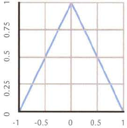
Tent filters derive their name from the tent-shaped function curve (see Figure 5.3). With such a graph, the x-axis represents the distance from a source pixel to the targeted pixel. The y-axis represents the weighted contribution of the source pixel. Hence, any pixel that is at a 0.5 pixel distance from the targeted pixel is weighted at 50%. Tent filters can be scaled to produce curve bases with different widths and thereby include a lesser or greater number of source pixels in the calculation. Tent filters are also known as triangle, bilinear, and Bartlett filters.
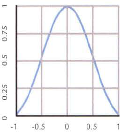
Cubic filters are a family of filters that employ a bell-shaped function curve (see Figure 5.4). Like tent filters, cubic filters base their weight on distance; however, the weighting is not linear. Cubic filters are well suited for the removal of high-frequency noise and are thus the default scaling method for Photoshop, After Effects, and Nuke. (When image processing is discussed, cubic filters are often referred to as bicubic as they must operate in an X and Y direction.)
One of the best ways to compare the qualities of various filters is to apply them to high-contrast edges that have gone through a rotation or an upscale. For example, in Figure 5.5, a white square is rotated, revealing the stair-stepping induced by a nearest neighbor filter. In addition, the subtle differences between tent and cubic filters are indicated by different degrees of softening.
Nuke offers additional convolution filters with which to apply transformations. They are discussed in the section "Transformations in Nuke" later in this chapter.
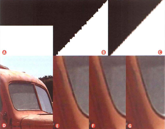
Figure 5.5. (A) Detail of a white square against a black background (B) The square rotated 45° through a nearest neighbor filter, with stair-stepping along the edge (C) The square rotated through a cubic filter (D) Detail of photo of a truck window (E) Photo upscaled by 500 percent with a nearest neighbor filter (F) Photo upscaled with a tent filter (G) Photo upscaled with a cubic filter. The white square image is included as filter.tif in the Footage folder on the DVD. The photo is included in the Footage folder as truck.tif.
After Effects and Nuke support multiple means to translate, scale, and rotate an image. In addition, both programs offer several ways to apply keyframe animation to the transformations. Each program provides editors to refine the resulting curves.
After Effects supports 2D and 3D transformations of 2D layers. You can add keyframes through the Timeline panel or the Effect Controls panel. You can edit the resulting curves in the viewer of the Composition panel or the Graph Editor, which supports both speed graph and value graph views.
By default, 2D transformations in After Effects occur around an anchor point. The anchor is indicated by a crosshair and is initially placed at the layer's center. You can reposition the anchor point by LMB+dragging with the Pan Behind tool (see Figure 5.6). To reset the layer so that it's centered on the anchor point, Alt+double-click the Pan Behind tool icon.
You can interactively move, scale, or rotate a layer in a viewer within the Composition panel. To move a layer, select the layer with the Selection tool and LMB+drag. You can also move the layer one pixel at a time by using the keyboard arrow keys while the layer is selected. To scale the layer, LMB+drag a point that falls on the layer's corner or edge. To rotate, choose the Rotation tool and LMB+drag.
For a higher degree of precision, you can enter transform values into the layer's Transform section within the layer outline of the Timeline panel (see Figure 5.7). The layer's Anchor Point, Position, and Scale properties are indicated by X, Y values. (The X and Y cells are unlabeled; the left cell is X and the right cell is Y.) Note that the values are based on the composition's current resolution with 0, 0 occurring at the upper-left corner of the layer. The layer's rotation is based on a scale of 0 to 359°. Any rotation below 0 or above 359 is indicated by the r ×prefix. For example, a rotation of −600 produces −1x −240 and a rotation of 500 produces 1×+140. To update a transform value, click the value cell and enter a new number. You can also interactively scroll through larger or smaller values by placing the mouse pointer over the value so that the scroll icon appears and then LMB+dragging left or right. By default, the Scale X, Y values are linked so that they change in unison. To break the link, deselect the Constrain Proportions link icon. You can enter negative values into the Scale X or Y cells, which serves as a handy way to invert a layer horizontally or vertically.

You can convert any 2D layer within After Effects to a 3D layer and thus gain an additional axis for transformation. To do so, toggle on the layer's 3D Layer switch (see Figure 5.8). Anchor Point Z, Position Z, Scale Z, Orientation, X Rotation, Y Rotation, and Z Rotation cells become available in the layer's Transform section (see Figure 5.7). (The Z cells are the furthest to the right.) In addition, an axis handle is added to the anchor point within the viewer of the Composition panel. By default, the x-axis is red and runs left to right, the y-axis is green and runs down to up, and the z-axis is blue and runs toward the camera (that is, toward the user). You can interactively position the layer by LMB+dragging an axis handle.
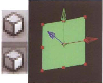
Figure 5.8. (Left) A 3D Layer switch toggled on in the layer outline (Right) A 100×100 layer's 3D transform handle
Orientation is controlled by X, Y, Z cells that use a scale of 0 to 359°. Changing the Orientation values rotates the layer; however, whole rotations below 0° or above 359° are not allowed to exist. If the layer reaches 360°, the value is reset to 0°. In contrast, X Rotation, Y Rotation, and Z Rotation operate with an r×prefix and are permitted to reach values below 0° or above 360°. It's not necessary to use both Orientation and X/Y/Z Rotation.
To move a layer away from the camera (as if "zooming out"), increase the Position Z value. To move the layer toward the camera (as if "zooming in"), decrease the Position Z value until it's negative. To offset the layer from its anchor point, increase or decrease the Anchor Point Z value so that it's no longer 0 (see Figure 5.9). If a layer is offset from its pivot, it rotates around the pivot as if it were a moon orbiting a planet. (Changing the Scale Z value has a similar effect, although negative values flip the axis handle by 180° in Y.)

Converting a layer to 3D does not create a new camera. Thus, any changes to the layer's transformations occur from a fixed viewpoint. To create a new camera, you must create a new Camera Layer. This process is detailed in Chapter 11, "Working with 2.5D and 3D."
To set a keyframe in After Effects, you must first toggle on the Stopwatch button beside the property you wish to animate (see Figure 5.10). A property is any layer or effects attribute that carries a channel or channels. Stopwatch buttons are accessible in the layer outline of the Timeline panel or in the Effect Controls panel. As soon as a Stopwatch button is toggled on, a keyframe is laid down for the property for the current frame. By default, keyframes are indicated on the timeline by a diamond-shaped dot (see Figure 5.10). At that point, new keyframes are automatically inserted for the property when there is a change in value.
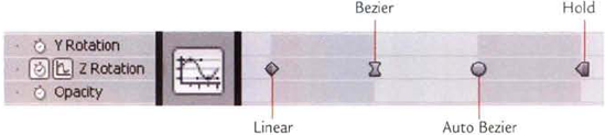
Figure 5.10. (Left) Stopwatch and Include This Property In Graph Editor Set buttons. Both buttons are toggled on. (Center) Graph Editor composition switch (Right) Keyframes displayed on the timeline
If a keyframe already exists for a particular frame, the keyframe is overwritten with a change in property value. You can update values by entering numbers into the property value cells, by adjusting the property sliders, or by interactively manipulating the layer in the viewer of the Composition panel. In addition, you can take the following steps to edit keyframes:
To delete a keyframe, select it and press the Delete key.
To select multiple keyframes, LMB+drag a marquee over them.
To delete all the keyframes for a property, toggle off the Stopwatch button.
To move a keyframe, LMB+drag it along the timeline.
To force the creation of a new keyframe when a value hasn't changed, move the current-time indicator (the vertical slider in the Timeline panel) to an appropriate frame, RMB+click over the property name in the layer outline, and choose Add Keyframe.
To enter specific values for a preexisting keyframe, select the keyframe, RMB+click, and choose Edit Value. Enter new values into the property dialog box and click OK.
To copy a selected keyframe, press Crtl+C, move the current-time indicator to a new frame, and press Ctrl+V.
To copy a set of selected keyframes from one property to another, press Crtl+C, highlight the name of the second property by clicking it in the layer outline, and press Ctrl+V. The second property can be part of the same layer or a completely different layer. The keyframes are pasted at the current frame, so it may be necessary to move the current-time indicator before pasting. Note that the paste will work only if the property has compatible channels. For example, you cannot copy keyframes from a Position property, which carries spatial X and Y data, to a Rotate property, which has temporal rotation data.
Recent releases of After Effects have added to the flexibility of the Graph Editor. To show the editor within the Timeline panel, toggle on the Graph Editor composition switch (see Figure 5.10). To display curves for a property, toggle on the Include This Property In Graph Editor Set button beside the property name in the layer outline (see Figure 5.10). The Graph Editor utilizes two types of data displays: value and speed. By default, the program chooses the type of display. However, you can change the display at any time by clicking the Choose Graph Type button and selecting Edit Value Graph or Edit Speed Graph from the menu (see Figure 5.11). If you select Edit Value Graph, you can ghost the speed graph within the editor by clicking the Choose Graph Type button and selecting Show Reference Graph. If you select Edit Speed Graph, Show Reference Graph will ghost the value graph.

Figure 5.11. (Bottom, Left to Right) Choose Graph Type button and its menu set; Show Transform Box When Multiple Keys Are Selected button; Snap button; Auto-Zoom Graph Height button; Fit Selection To View button; Fit All Graphs To View button
The After Effects value graph is similar to the curve editor used in Nuke or other 3D programs such as 3ds Max or Maya. Time is mapped to the horizontal x-axis and value is mapped to the vertical y-axis. If curves are not immediately visible within the Graph Editor, you can frame them by clicking the Fit All Graphs To View button (see Figure 5.11).
Many properties, including Scale, Rotate, and Opacity, allow you to manipulate their tangent handles interactively. Tangent handles are referred to as direction handles in the After Effects documentation. Tangent handles shape the curve segments as they thread their way through the keyframes. You can change tangent types by selecting keyframes and clicking one of the tangent type buttons at the bottom of the editor (see Figure 5.12).

In addition, you can change the tangent types by RMB+clicking over a keyframe in the Graph Editor or the Timeline panel and choosing Keyframe Interpolation. Within the Keyframe Interpolation dialog box, the Temporal Interpretation menu controls tangent types within the Graph Editor. By default, keyframes are assigned Linear tangents. That is, the curve runs in a straight line between keyframes. Here is a list of the other tangent types:
Hold creates a stepped curve where values do not change until a new keyframe is encountered. Hold tangents are indicated on the timeline by an icon that has a squared-off side (see Figure 5.10 earlier in this section).
Bezier creates a spline curve that attempts to thread each keyframe smoothly. Bezier tangent handles are broken; that is, you can select and LMB+drag the left and right side of a tangent handle independently. Bezier tangents are indicated on the timeline by an hourglass-shaped icon (see Figure 5.10).
Continuous Bezier also creates spline curves. However, the tangent handles are not broken. Continuous Bezier tangents are indicated on the timeline by an hourglass-shaped icon.
Auto Bezier automatically massages the shape of the curve to maintain smoothness. This occurs when the keyframe value is changed through a property value cell, through a property slider, or through the Edit Value dialog box. If the tangent handle is interactively adjusted through the Graph Editor, the tangent type is instantly converted to a Continuous Bezier. Auto Bezier tangents are indicated on the timeline by a circular icon (see Figure 5.10).
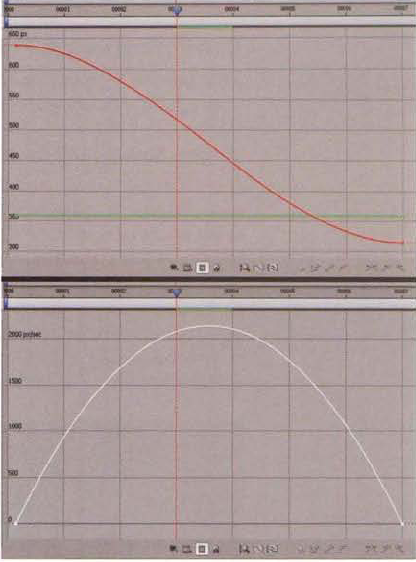
The speed graph, when compared to the value graph, is less intuitive. Whereas the value graph shows a change in property value over time, the speed graph shows the rate of change for a property value. Hence, the y-axis of the speed graph represents the formula value/second. As a simple comparison, in Figure 5.13, a 100×100 solid is animated moving from the right side of the screen to the left side. On frame 1, the solid has a Position value of 640, 360. At frame 7, the solid has a Position value of 300, 360. If the Graph Editor is set to the value graph view, the Position X curve makes a downward slope, which indicates that the X value is decreasing over time. The Position Y curve, in contrast, is flat, indicating that there is no change to the Y value. If the editor is switched to the speed graph view, the Position X and Y curves become stepped and overlap. Although the solid continues to move in the X direction, the rate of change does not fluctuate. That is, over each of the 7 frames, the solid is moving 1/7 the total distance.
To give the speed graph view curves some shape, you have to change the speed of the solid. Adding an ease in or ease out is a quick way to accomplish this. To add an ease in and ease out, select the curve in the speed graph view and click the Easy Ease button at the bottom of the Graph Editor (see Figure 5.12 earlier in this section). This bows the shape of the Position curve in the speed graph view (see Figure 5.14). This equates to the solid moving slowly at the start and at the end of the animation but rapidly through the middle. The height of the curve for a particular frame indicates the speed of the solid. For example, at frame 1, the solid is moving approximately 925 pixels per second. At frame 4, the solid is moving at approximately 2,105 pixels per second. Again, the y-axis of the speed graph represents value/second or, in this case, pixels moved/second. The slope of the curve, therefore, represents the change in speed. A steep slope indicates a rapid change in speed while a shallow slope indicates an incremental change in speed.

Figure 5.13. (Top) Solid and its motion path in the viewer. (Center) Value graph view. The red curve is Position X. (Bottom) Speed graph view. A sample After Effects project is included as speed_flat.aep in the Tutorials folder on the DVD.
If you switch the Graph Editor to the value graph view, the X curve takes on a more traditional shape. With the application of the Easy Ease button, which creates an ease in and ease out, the slope at the curve's start and end is shallow, indicating an incremental change in value (see Figure 5.14). The center of the curve has a steep slope, indicating a rapid change in value.
To manipulate tangent handles within the speed graph or the value graph view, select a keyframe and LMB+drag the corresponding handle. You can change the length of a handle, and therefore influence the curve shape, by pulling the handle further left or right. If the tangent is set to Bezier and you are using the speed graph view, you can move the left and right side of the tangent handle away from each other vertically. Such a separation can create a significant change in speed over one frame. In the value graph view, you can rotate the tangent by pulling a tangent handle up or down. However, tangent handles are not available to Linear keyframes in the value graph view. In addition, spatial properties, such as Anchor Point of Position, do not make tangent manipulation available to the value graph view; nevertheless, the tangents are available in the speed graph view or through the overlay of the viewer (see the section "Editing Curves in the Viewer"). Note that Position X, Y, and Z keyframes are linked. Although X, Y, and Z each receive their own curve, their keyframes cannot be given unique frame values or be deleted individually. After Effects CS4 avoids this limitation by allowing you to keyframe each channel separately.
Whether you choose to work within the speed graph view or the value graph view, there are a number of editing operations you can apply within the Graph Editor:
To add a keyframe, Ctrl+Alt+click on a curve.
To delete a selected keyframe, press the Delete key.
To move a selected keyframe, LMB+drag.
When multiple keyframe points are selected, a white transform box is supplied if the Show Transform Box When Multiple Keys Are Selected button is toggled on (see Figure 5.11 earlier in this chapter). You can LMB+drag the box left or right and thus move the keyframes as a unit over time. You can LMB+drag the box up or down and thus change the keyframe values. You can scale the keyframes as a unit by LMB+dragging an edge handle.
You can apply an automatic ease out by selecting a keyframe and clicking the Easy Ease Out button at the bottom of the Graph Editor (see Figure 5.12 earlier in this chapter). To apply ease in, click the Easy Ease In button.
As a bonus, you can edit keyframes and tangent handles interactively in the viewer of the Composition panel. Within the viewer, keyframes are represented by hollow boxes and the motion path of the layer is indicated by a line running through the keyframes (see Figure 5.13 earlier in this chapter). To select a keyframe, click on its box. To move a selected keyframe, LMB+drag. Any changes applied in the viewer are automatically applied to curves within the Graph Editor.
Tangents found within the viewer have their own set of interpolation properties. By default, the tangents are linear. However, you can change the type by selecting a keyframe, RMB+clicking, choosing Keyframe Interpolation, and changing the Spatial Interpolation to Bezier, Continuous Bezier, or Auto Bezier. The Spatial Interpolation settings do not affect the tangent setting for the curves within the Graph Editor. However, if you move the tangent handles within the viewer, the curves in the Graph Editor automatically update.
Nuke provides transformation capabilities through specialized nodes. In addition, the program allows keyframe and curve manipulation through its Curve Editor pane.
In order to move, scale, rotate, or skew the output of a node, you must add a Transform node (Transform → Transform or the default T hotkey). Translate X and Y cells, as well as Rotate, Scale, and Skew sliders, are provided by the Transform node's properties panel (see Figure 5.15). You can also interactively manipulate the resulting transform handle in a viewer. LMB+dragging within the handle circle moves the image. LMB+dragging a point on the circle scales the image in that particular direction. LMB+dragging an arc segment on the circle scales the image in both directions. LMB+dragging the short vertical lines that extend past the top or the bottom of the circle skews the images (turns it into a trapezoidal shape). LMB+dragging the long horizontal line to the right of the circle rotates the image.
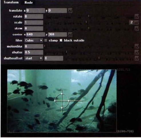
Figure 5.15. (Top) Transform node's properties panel (Bottom) Interactive transform handle in a viewer.
The Transform node provides several interpolation filters with which to adjust the quality of averaged pixel values. You can select a filter type by changing the Filter menu in the Transform node's properties panel. Brief descriptions follow:
Cubic is the default filter, which offers the best combination of quality and speed. For more information on cubic and similar filters, see the section "Interpolation Filters" earlier in this chapter.
Impulse creates a nearest neighbor style filter whereby the new pixel receives the value of the original pixel or, in the case of scaling, the value of the closest original pixel. The filter takes a minimal amount of computational power but leads to blockiness (see Figure 5.16).
Keys uses a bell-shaped function curve but introduces subtle edge sharpening (see Figure 5.16). The Keys function curve is allowed to dip into negative values along the bell base.
Simon is similar to Keys but produces medium-strength sharpening.
Rifman is similar to Keys but produces strong sharpening.
Mitchell is similar to both Cubic and Keys in that it produces smoothing with a very subtle degree of edge sharpening.
Parzen produces the second strongest smoothing among Nuke's convolution filters (see Figure 5.16). Its function curve is a shortened bell curve.
Notch produces the greatest degree of smoothing due to the flattened top of its bell curve.

Aside from the Transform node, Nuke offers several specialty transformation nodes, all of which are found under the Transform menu:
TransformMasked operates in the same fashion as the Transform node but allows the transformation to occur on a particular channel. For example, you can change the TransformMasked node's Channels menu to Alpha and change the Translate X value to −2, thus subtly shifting the alpha matte to one side.
Position simply translates the image in the X or Y direction. The node automatically streaks the boundary pixels of the image to disguise any gaps that are opened as the image is moved aside.
Mirror flips the image in the horizontal and/or vertical directions.
CameraShake adds its namesake to a node's output (see Figure 5.17). This is useful for re-creating earthquakes, shock waves, handheld camerawork, and the like. The Amplitude slider controls the strength of the shake. The Rotation slider, when raised above 0, inserts rotation along the camera's z-axis. The Scale slider, when above 0, moves the image either closer to or farther from the viewer along the camera's z-axis. The Frequency slider controls the lowest frequency and thus the "graininess" of the underlying noise function. Large Frequency values lead to a small "grain," which causes the shake to be violent and chaotic. Small values lead to large "grains," which cause the shake to be slow and smooth (similar to the float created by a Steadicam). The Octaves cell controls the complexity of the underlying noise. With each whole value increase of the Octaves cell, an additional frequency of noise is layered on the base noise and the more complex and seemingly random the shaking becomes. The CameraShake node automatically adds 2D motion blur to the image; the strength of the blur corresponds to the distance the image is moved for a frame. In addition, the node automatically streaks the boundary pixels of the image to disguise any gaps that are opened as the image is moved aside.
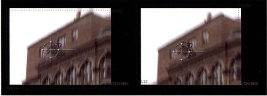
Figure 5.17. Two frames showing the movement and motion blur introduced by a CameraShake node. The squiggly line in the center is the motion path created by the node for a 30-frame animation. A sample Nuke script is included as camerashake.nk in the Tutorials folder on the DVD.
The LensDistortion node creates the subtle spherical distortion of real-world lenses. This is useful for matching live-action footage when motion tracking. The LenDistortion node is detailed in Chapter 10, "Warps, Optical Artifacts, Paint, and Text." The SphericalTransform node, on the other hand, is designed for HDRI mapping, which is discussed in Chapter 12, "Advanced Techniques."
To set a keyframe, click an Animation button (with a picture of a curve) and choose Set Key from the menu (see Figure 5.18). Animation buttons are provided for any parameter that supports an animation channel. You can also key all the available parameters for a node in one step by RMB+clicking over an empty area of a properties panel and choosing Set Key On All Knobs. (Each keyable parameter is referred to as a knob.) Once a parameter has been keyed, its corresponding numeric cell or check box turns cyan. In addition, cyan tick marks are added to the viewer timeline to indicate the presence of keyframes. (Keyframes are placed at the current frame, so it's important to check the timeline first.) As soon as one keyframe has been set for a parameter, any change in value for that parameter automatically creates a new keyframe. You can delete a keyframe by clicking an Animation button and choosing the Delete key from the menu. You can destroy all the keyframes for a parameter by clicking the corresponding Animation button and choosing No Animation from the menu.
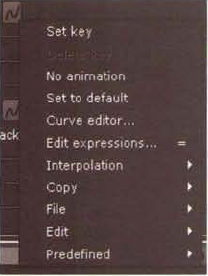
To edit keyframes and corresponding curves, you can use Nuke's Curve Editor. To launch the editor, click an Animation button for a parameter that carries animation and choose Curve Editor from the menu. The Curve Editor integrates itself into a pane beside the Node Graph. The left column of the editor displays all the parameters for the node that carry keyframes. If a parameter has a single channel, such as Rotate or Skew, only one matching curve is indicated by a : symbol. If a parameter has more than one channel, the matching curves are listed by their names. For example, Translate lists x: and/or y: curves, while Scale lists w: and/or h: curves (see Figure 5.19). To view all the curves of a parameter, click the parameter name. To view specific curves, Shift+click the curve names. You can use the standard camera controls to zoom in or out (Alt+MMB) and scroll (Alt+LMB) within the curve grid. To frame selected curves automatically, press the F key.

Here are basic steps to take to select, edit, and delete keyframes and curves:
To select a keyframe point, click it or LMB+drag a marquee box around it.
To select multiple keyframe points, Shift+click them or LMB+drag a marquee box around them.
To move a selected keyframe, LMB+drag. By default, the keyframe is locked to either its current frame or current value, depending on the direction you initially drag the mouse. To move the selected keyframe freely, Crtl+LMB+drag.
To move a selected keyframe to a specific location, RMB+click and choose Edit → Move. In the Move Animation Keys dialog box, enter specific values in the X and/or Y cells and press OK (see Figure 5.20). You can also enter a specific value for the tangent handle slope. Slope, as a term, describes the steepness or incline of a straight line. In Nuke, tangent slopes are measured as a θ (theta) angle. When you select a keyframe, the θ measurement for the right slope is displayed by the right side of the tangent handle (see Figure 5.20). In terms of the Move Animation Keys dialog box, you can enter values into the (Right) Slope or Left Slope cells. If the values of the two slopes are different, the tangent handle is automatically broken; thereafter, you can move each side independently. Slope values are either negative or positive. The range is dependent upon the position of the keyframe on the curve, the type of tangent interpolation, and its proximity to other keyframes. The program automatically clips slope values that are too small or too large. More directly, you can enter a right slope value by clicking the slope readout beside the tangent handle and entering a new value into the cell that appears.
To assign a keyframe to a specific frame, select the keyframe and click the × portion of the numeric readout that appears beside it. Enter a value into the cell that opens.
To assign a keyframe to a specific value, select the keyframe and click the y portion of the numeric readout that appears beside it. Enter a value into the cell that opens.
To delete selected keyframe(s), press the Delete key.
To insert a new keyframe along a curve's current path, Ctrl+Alt+click the curve at the point where you want a new keyframe.
To insert a new keyframe at a point that lies off the curve's path, click the curve so that it turns yellow, then Ctrl+Alt+click at a point off the curve. A new keyframe is inserted at that point and the curve is reshaped to flow through the new keyframe.
To copy a keyframe, select it, RMB+click, and choose Edit → Copy → Copy Selected Keys. Select a different curve through the left column. RMB+click and choose Edit → Paste.
To impose the shape of one curve onto a second curve, select a curve, RMB+click, and choose Edit → Copy → Copy Curves. Select a different curve through the left column. RMB+click and choose Edit → Paste.
To reverse a curve, select the curve (or a set of keyframes), RMB+click, and choose Predefined → Reverse. The curve is reversed and its original position is indicated by a dashed line. You can undo the reverse by choosing Predefined → Reverse again.
To flip a curve vertically, choose Predefined → Negate.
To smooth a curve automatically, select a set of keyframes, RMB+click, choose Edit → Filter, enter a value into the No. Of Times To Filter cell of the Filter Multiple dialog box, and click OK. The higher the value, the stronger the averaging will be and the flatter the curve will get in that region.
You can create evenly spaced keyframes along a curve by selecting the curve so that it turns yellow, RMB+clicking, and choosing Edit → Generate Keys from the menu. In the Generate Keys dialog box, choose Start At and End At frames and an Increment value. If you wish for the new keyframes to have a specific value, enter a number in the curve name cell. For example, if you select the Y curve of a Translate parameter, the curve name cell is y: and the cell value is y. If you leave y in the cell, the new keyframes will be spread along the curve's current path. If you change y to a particular value, such as 1, the new keyframes will appear with that value and the old curve path is altered.

When a keyframe is selected, tangent handles automatically appear. You can LMB+drag any handle to change the curve shape. In addition, Nuke offers seven tangent types that you can select by RMB+clicking and choosing Interpolation → interpolation type from the menu. While Linear and Smooth types are identical to those used by other compositing and 3D programs, several types are unique (at least in name):
Constant creates a stepped curve. There is no change in value until the next keyframe is encountered (see Figure 5.21).
Catmull-Rom matches the tangent slope to a slope created by drawing a line between the nearest keyframe to the left and right. This generally leads to a subtle improvement in the roundness to curve peaks and valleys (see Figure 5.21).
Cubic aligns the tangent handle to the steepest side of the curve as it passes through the keyframe. This prevents the appearance of sharp peaks within the curve (at least where the cubic tangents are), but it may also lead to the curve shooting significantly past the previous minimum or maximum values (see Figure 5.21).
Horizontal forces the tangent handle to have 0 slope. This may produce results similar to unadjusted Smooth tangents (see Figure 5.21).
Break snaps the tangent in half so that each side can be adjusted independently.

Although compositing normally involves captured footage of some sort, it's possible to create animation with static images. After Effects and Nuke offer a wide array of keyframing and curve editing tools to achieve this effect.
Editing animation curves within the After Effects Graph Editor gives you a great degree of control. For example, in this tutorial the editor will allow you to give a static ball a believable series of bounces.
Create a new project. Choose Composition → New Composition. In the Composition Settings dialog box, set the Preset menu to Film (2K). Set Duration to 36, Start Frame to 1, and Frame Rate to 30. Import the
floor.tgaandball.tgafiles from the Footage folder on the DVD. Interpret the alpha on the ball.tga file as Premultiplied.LMB+drag
ball.tgafrom the Project panel into the layer outline of the Timeline panel. Select the Pan Behind tool (Y is the default hot key). LMB+drag the anchor point for theball.tgalayer so that it rests at the center of the ball (see Figure 5.22). A centered anchor is necessary for any rotational animation. The Anchor Point property, in theball.tgalayer's Transform section, should be approximately 1060, 710 once the anchor point is centered. LMB+dragfloor.tgafrom the Project panel to the bottom of the layer outline. The CG ball is thus composited over the top of a floor photo.Move the timeline to frame 1. Expand the Transform section of the
ball.tgalayer in the layer outline. Set the Scale to 120%. Set the Rotation to −25. Set the Position to 1160,−80. This places the ball out of frame at the upper right. Toggle on the Stopwatch buttons beside the Position, Scale, and Rotation properties. Keyframes are set on the timeline.Move the timeline to frame 36. You can interactively drag the current-time indicator in the Timeline panel or enter the frame number in the Current Time cell at the top left of the layer outline. Change Position to 875, 1000, Scale to 125%, and Rotation to 50. Because a key has already been set on the properties, new keyframes are automatically laid down with the change in values. As soon as two keyframes exist, a motion path is drawn in the viewer for the ball.
Move the timeline to frames 6, 11, 16, 21, 26, and 31, interactively positioning the ball as you go. The ball should bounce three times; that is, the ball should touch the ground at frames 6, 16, 26, and 36 while hitting the peak of a bounce at frames 11, 21, and 31. Each bounce should be shallower than the previous one. You can adjust the position of the keyframes in the viewer by LMB+dragging a keyframe point. Use Figure 5.23 as a reference for the shape of the motion path. To smooth the peak of each bounce, select a keyframe for frame 11, 21, or 31 and LMB+drag the displayed tangent handle. You can lengthen a tangent handle by LMB+dragging it left or right. If it's difficult to see the tangent handle, set the viewer's Magnification Ratio Popup menu to zoom in closer. To make sharp turns with the motion path at the points that the ball touches the ground, shorten the tangent handles for frames 6, 16, and 26.
Use the Time Controls panel to play back the timeline. Make sure that the playback occurs at approximately 30 fps. The Info panel will display the playback rate and whether or not it is real time. Adjust the keyframes and motion path of the ball layer until you're satisfied with the overall motion. For additional information on keyframe and curve editing, see the section "Using the Graph Editor" earlier in this chapter.
At this stage, the ball is increasing in scale as it bounces toward the foreground. You can refine the scale transition in the Graph Editor. In the layer outline, toggle on the Include This Property In The Graph Editor Set button beside the Scale property. Toggle on the Graph Editor composition switch at the top-right of the layer outline. The Graph Editor opens in the Timeline panel. Click the Choose Graph Type And Options button, at the bottom of the Graph Editor, and choose Edit Value Graph. Click the Fit All Graphs To View button to frame the Scale curve. Since the Scale property's Constrain link remains activated, only one curve is supplied for Scale X and Y. Insert keyframes at frames 6, 11, 16, 21, 26, and 31. To insert a new keyframe, Ctrl+Alt+click the curve. Interactively move the keyframes for frames 6, 16, and 26 to make the scale slightly smaller. This will give the illusion that the ball gets closer to the camera at the peak of each bounce. Use Figure 5.24 as a reference for the shape of the curve. You can add smoothness to the curve by manipulating the tangent handles. To do so, LMB+drag to select all the keyframes, RMB+click over a keyframe, and choose Keyframe Interpolation from the menu. In the Keyframe Interpolation dialog box, set the Temporal Interpolation menu to Bezier and click OK. To move a tangent handle, select a keyframe in the Graph Editor and LMB+drag the left or right tangent handle point.
At this stage, the ball feels disconnected due to a lack of shadow (see Figure 5.25). You can create a shadow using the duplicate of the ball layer with Blur and Brightness & Contrast filters. This process, along with the application of artificial motion blur and camera move, will be addressed in the Chapter 6 After Effects follow-up tutorial. In the meantime, save the file for later use. A sample After Effects project is included as
ae5.aepin the Tutorials folder on the DVD.
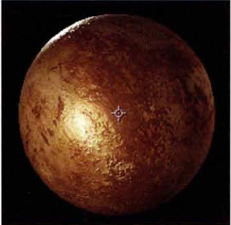


Figure 5.25. The initial composite. A shadow will be added in the Chapter 6 After Effects follow-up tutorial.
Editing animation curves within the Nuke Curve Editor gives you a great degree of control. For example, in this tutorial the editor will allow you to give a static ball a believable series of bounces.
Create a new script. Choose Edit → Project Settings. Change Frame Range to 1, 36 and Fps to 30. With the Full Size Format menu, choose 2k_Super_35(Full-ap) 2048×1556. In the Node Graph, RMB+click, choose Image → Read, and browse for the
floor.tgafile in the Footage folder on the DVD. With no nodes selected, RMB+click, choose Image → Read, and browse for theball.tgafile in the Footage folder on the DVD. In the Read2 node's properties panel, select the Premultiplied check box.With the Read2 node selected, RMB+click and choose Transform → Transform. With no nodes selected, RMB+click and choose Merge → Merge. Connect input A of the Merge1 node to the output of the Transfrom1 node. Connect input B of the Merge1 node to the output of the Read1 node. Connect the output of the Merge1 node to a viewer. A CG ball is composited over the top of a floor photo. Before you are able to animate, however, it's necessary to center the ball's transform pivot. In the Transform1 node's properties panel, set the Center X cell to 1062 and the Center Y cell to 850 (see Figure 5.26). This centers the transform handle over the ball.
Move the timeline to frame 1. In the Transform1 node's properties panel, set Scale to 1.20. Set Rotation to 50. Set the Translate X and Y cells to 26, 760. This places the ball out of frame. Click the Animation button beside the Translate parameter and choose Set Key. The cell turns cyan and a cyan line appears over frame 1 on the timeline of the viewer. Repeat the Set Key process for the Scale and Rotate parameters.
Move the timeline to frame 35. Change the Translate X and Y cells to −196, −196. This moves the ball to the center of the frame. Set the Rotate slider to −25. Set the Scale slider to 1.25. New keyframes are automatically placed on the timeline. As soon as two keyframes exist for the Translate parameter, a motion path is drawn in the viewer.
Move the timeline to frames 5, 10, 16, 21, 26, and 31, interactively positioning the ball as you go. The ball should bounce three times; that is, the ball should touch the ground at frames 5, 16, 26, and 35 while hitting the peak of a bounce at frames 10, 21, and 31. Each bounce should be shallower than the previous one. Use Figure 5.27 as reference for the initial shape of the motion path.
Check the viewer's Desired Playback Rate cell. It should say 30 by default. Play back the timeline with the viewer Play button. Watch the Desired Playback Rate cell to make sure the playback is approximately 30 fps. If the playback is too slow, then set the viewer's Downrez menu to a value that allows the proper playback speed. (For more information on critical viewer settings, see Chapter 1.) At this point, the bouncing may appear somewhat mechanical or as if the ball is attached to an elastic string. The duration for which the ball hangs in the air or touches the ground is not ideal. Due to the default Smooth tangent types, there are sharp corners as the ball peaks. In addition, there is an ease in and ease out as the ball nears the ground. To address this, adjust the keyframes and tangent types in the Curve Editor.
In the Transform node's properties panel, click the Animation button for an animated parameter and choose Curve Editor from the menu. The Curve Editor opens in a pane beside the Node Graph. Click the y: below the word Translate in the left column to show the Translate Y curve. Press the F key while the mouse pointer is over the Curve Editor to frame the curve. To improve the arc at each bounce peak, interactively manipulate the tangents for keyframes at 10, 21, and 31. You can move a tangent handle by clicking on a keyframe and LMB+dragging the left or right tangent handle point. The motion path in the viewer will update as the tangent handles are manipulated.
To prevent the ease in/out as the ball touches the ground, Shift+select the keyframes at 5, 16, and 26, RMB+click over a keyframe, and choose Interpolation → Break. This breaks each tangent in half. Adjust the left and right side of each tangent handle to remove the ease in and ease out. When you adjust the tangents' handles at the point the ball touches the ground, the tops of each bounce gain additional roundness, which equates to a slightly longer "hang time" for the ball (see Figure 5.28). The only keyframe that doesn't gain additional roundness is the one resting at frame 1. Select the frame 1 tangent handle and adjust it so that the curve no longer makes a linear path from frames 1 to 5.
At this point, there may be a slight bend in the ball's motion path as the ball descends from its bounce (see Figure 5.29). This is due to the X curve remaining in its initial state. Select the x: below the word Translate in the left column of the Curve Editor. Press the F key to frame the X curve. Rotate the tangent handles for frames 5, 16, and 26 until the bend disappears (see Figure 5.29). Play back the timeline. Continue to refine the tangent rotations for all the keyframes of both the X and Y curves.
From frame 1 to frame 35, the ball changes from a scale of 1.2 to 1.25. This slight increase will help to create the illusion that the ball is getting closer to the camera. You can exaggerate this scale shift by also changing the ball scale between the peaks and valleys of each bounce. To do so, click the w: below the word Scale in the left column of the Curve Editor. Press the F key to frame the W curve. (Since the scale occurs equally for the width and height of the ball, only the W curve is provided.) Move the timeline to frame 5. In the Transform1 node's properties panel, click the Scale parameter's Animation button and choose Set Key. This places a new keyframe on the curve without disturbing its current value. Repeat the process for frames 10, 16, 21, 26, and 31. In the Curve Editor, move the keyframes so that the scale is slightly larger at the bounce peaks and slightly smaller at the point where the ball touches the ground. Use Figure 5.30 as reference.
At this point, the ball feels disconnected due to a lack of shadow. You can create a shadow using the CG render of the ball with additional Transform, Grade, and Blur nodes. This process, along with the application of artificial motion blur and camera move, will be addressed in the Chapter 6 Nuke follow-up tutorial. In the meantime, save the file for later use. A sample Nuke script is included as
nuke5.aepin the Tutorials folder on the DVD.
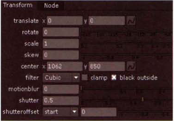


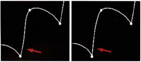
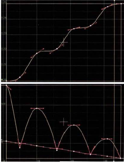
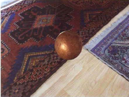
Figure 5.31. The initial composite. A shadow will be added in the Chapter 6 Nuke follow-up tutorial.
In 1998, Erik Winquist graduated from the Ringling School of Art and Design with a degree in computer animation. Shortly thereafter, he joined Pacific Data Images as a digital artist. In 2002, he joined Weta Digital as a compositor. After a six-month stint at ILM as a compositor on Hulk, Erik returned to Weta to serve as a compositing supervisor on I, Robot; King Kong; X Men: the Last Stand; and Avatar. He was also the visual effects supervisor on The Water Horse and Jumper.

Erik Winquist (Image courtesy of Weta Digital)
Weta was formed in 1993 by New Zealand filmmakers Peter Jackson, Richard Taylor, and Jamie Selkirk. It later split into two specialized halves: Weta Digital for digital effects and Weta Workshop for physical effects. Weta Digital has been nominated for five visual effects Oscars and has won four.
(Weta Digital keeps a core staff of 40 compositors but expands for large shows.)
LL: What is the main compositing software used at Weta Digital?
EW: We've been a Shake house since [The Lord of the Rings: The Fellowship of the Ring]. In 2004, during work on I, Robot, we started evaluating Nuke, which was used fairly extensively on King Kong as an environments tool and has been slowly gaining favor as a compositing package among the compositing department....
LL: What would be the greatest strength of either Shake or Nuke?
EW: With Shake, hands down, it's the user base. It's that package that everyone knows and is easiest to hire artists [for] on short notice... We also have a large collection of in-house plug-ins that has been written over the years... Nuke has been a bit more foreign at first glance, but once you get into it, its speed and toolset is just a boon for this increasingly 3D "two-dimensional" work that we do each day. It's definitely a compositing package that has evolved over the years in a production environment. The recent inclusion of Python scripting support has been really great for scripting tools that would otherwise require compiled solutions...
LL: In your experience, do you prefer working with proprietary, in-house compositing software or off-the-shelf, third-party software?
EW: The most flexible solution seems [to be] a third-party application [that] is expandable via software developers' kits (SDKs). That way, you get the benefit of using a tool [that] lots of people will already know but at the same time have the ability to write custom in-house tools to work best with your specific pipeline.
LL: What type of workstations do Weta compositors use?
EW: All of the compositors here are working on dual quad-core Intel boxes running Kubuntu Linux with 8 gigabytes of RAM. We generally don't do fast local storage here, as everything is served from network filers. Most artists have two machines at their desks for better multitasking.
LL: What resolutions do you normally comp at?
EW: That depends on the project really, but the vast majority of shows that have come through Weta have been shot Super35, with a scanning full aperture resolution of 2048×1556 and a 16×9 delivery resolution of 2048×1157. Current HD shows and are being ingested from tape at 1920×1080. We recently completed a special venue project which had a 6:1 delivery ratio with source plates shot on a special tiled rig using three Red One cameras shooting simultaneously.
LL: How is it to work with Red One footage?
EW: There have been a couple shows we've worked on recently [that] used the Red camera for at least a handful of plates, often for pickup shoots. The trouble I've seen early on is that none of the plates were coming in with any consistent color space from show to show, or even shot to shot. For the aforementioned special venue project shot on Red... the images were shot and converted correctly from RAW to linear float EXRs, which were then a breeze to comp with.
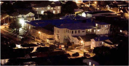
The Weta Digital facilities tucked into a quiet corner of Wellington (Image courtesy of Weta Digital)
LL: Does 35mm footage suffer from any quirks not present with high-definition digital video footage? How about vice versa?
EW: 35mm film still gives your loads more dynamic range than the HD footage that's come across our workstations. Whereas scanned film negative can give you almost four stops above reflected white, the Red footage is only about one stop above. Anything brighter than that is clipped. Where 4:4:4 HD is proving nice is in its lack of film grain and what that can do for extracted keys. Edges and highlights don't suffer from emulsion halation like film.
Darren Poe began his career as a graphic designer and video postproduction artist. He joined Digital Domain in 1996 as a 3D effects artist. After working on The Fifth Element and Titanic, he went on to specialize as a compositor. His film roster has since included such features as Fight Club, Daredevil, The Day After Tomorrow, Charlie and the Chocolate Factory, Pirates of the Caribbean: At World's End, and Speed Racer. He currently serves as a digital effects supervisor.

Darren Poe (Image courtesy of Digital Domain)
Digital Domain was founded in 1993 by visual effects pioneers Scott Ross, James Cameron, and Stan Winston. The studio has gone on to win seven visual effects and scientific achievement Oscars with its credits exceeding 65 feature films and scores of television commercials.
LL: Digital Domain developed Nuke in-house. Do you currently use the publicly available commercial version or a custom variation?
DP: Since The Foundry took over the development of Nuke, we're basically using whatever their latest beta is, at least on the show I'm on right now. We have our own in-house custom tools, which are more like plug-ins to Nuke as opposed to variants on the actual build of Nuke itself. (Nuke stands for "New Compositor.")
LL: Do you use any other compositing programs?
DP: We do have Shake and will use it in certain circumstance, but 99.9 percent of what we do is Nuke.
LL: Have you used any other packages over the years?
DP: I should go back and say that I'm one of the last people who uses Flame, at least on the feature side. I sometimes forget that I do that. These days, it's primarily used in commercial production. It's a known quantity. Agencies come in knowing what the box can do.
LL: Do you prefer using in-house, proprietary software or off-the-shelf, third-party software?
DP: There are advantages both ways. If you use commercially available software, it broadens the range of people you can bring in to work on a show. One of the things that has changed a lot in the industry is that the model of hiring people has come much closer to the duration and needs of the show. So, you really need to be able to find skilled people who can start immediately—where you don't have that year of ramp-up and training or mentoring....
LL: Is that wide-spread in Los Angeles—hiring a compositor for the duration of a single show or project?
DP: That's pretty much how most places operate. People who have the broadest set of skills with the latest commercial software put them at a great advantage to come in without having to completely learn a new system. But at the same time, with the exception of Nuke, there are a lot of limitations to commercial software that's developed outside of a production context. We build a lot of tools and knowledge over the years based on things that happened on shows and needs that have come up, so that's where the proprietary part of it becomes very important.
LL: As a compositor, what kind of workstation do you use?
DP: We're using Linux. Typically [dual quad-core] machines....usually a dual monitor type of set up.
LL: What resolutions do you normally comp at?
DP: It's completely dependent on the show. We've done a lot of HD (1920×1080) recently (for example, 2012, which is shot digitally). Right now, we're doing a show that's 4K, so it really runs the gambit.

Inside the modern Digital Domain facility. The arced structure to the right is a large conference room designed by architect Frank Gehry. Miniatures from The Fifth Element and Apollo 13 sit close by. (Image courtesy of Digital Domain)
LL: Have you worked with Red One footage?
DP: We just did some tests with the Red camera....it's still early [in the testing process]. I don't think any show is really using it—like actually going out and shooting full elements....
LL: So it's still very common to shoot 35mm or VistaVision?
DP: It's still very common, although HD is making huge inroads (Speed Racer was shot on HD).
LL: Is it common to work with bluescreen or greenscreen?
DP: Percentage-wise, it's probably less than it has been in the past. As an industry, [we've] moved to a point where rotoscoping and other ways of extraction are seen as possible or even desirable.
LL: What do you use to pull the keys?
DP: Basically, we use Nuke. What's in Nuke is Primatte, Keylight, and Ultimatte.... all the main [keyers]....
LL: Do you see more and more "dirty" plates? That is, are visual effects plates now being shot with no blue- or greenscreen at all, preferring to let the compositing team to do whatever they need to do to make the effect work?
DP: Definitely. The cost benefit of properly setting up a shoot with an evenly lit greenscreen can be poor when compared to having the compositing team fix the shot.
LL: Do you rotoscope in house?
DP: We roto in-house.... We basically operate a pool [of rotoscopers] that fluctuates in size depending on the needs of various shows. They [work] across the different shows.