
"Tracking is something that a Flame artist will do every day, be it making a garbage mask to follow a simple move or tracking a new head onto someone".
Masking, which is the process of creating mattes, is an inescapable step for complex compositing. Masking may be as simple as drawing a spline path with a dedicated masking tool. However, the task becomes more complicated when the matte needs to travel and the masking turns into rotoscoping. Motion tracking, on the other hand, requires the software to track features or patterns with a piece of footage and convert that information to animation curves. Once the curves exist, they may be used to apply motion to a different layer or input, remove the jitter from a shaking camera, or change the perspective of an element so that it fits a scene with a moving camera. Although the motion tracking process is semi-automated, special care must be taken when positioning tracking points. To help you practice this technique, as well as various masking and rotoscoping tasks, a new tutorial is added to this chapter. In addition, you'll have to chance to revisit the tutorial from Chapter 3.
Although the terms matte and mask are often used interchangeably, they refer to two separate parts of the same process. As discussed in Chapter 3, a matte establishes pixel opacity for a digital image and is thus needed to composite multiple images together. Matte values, as expressed by an alpha channel, range from 0 to 1.0 on a normalized scale. Hence, a matte is black and white, with additional shades of gray to establish tapering transparency.
A mask, in comparison, is the device that creates the matte. For example, the Pen tool in After Effects creates a closed spline path. Pixels falling inside the path are assigned an alpha value of 1.0, while pixels falling outside the path are assigned an alpha value of 0. The path is a mask; the resulting alpha channel is a matte. In contrast, many Nuke nodes carry a Mask parameter that establishes what input will be used as a matte. Despite the confusion in terminology, masking may be considered the process of creating a matte.
Rotoscoping is the process by which animators trace over live-action footage one frame at a time. The rotoscope process was developed by Max Fleischer, who patented the idea in 1917. Originally, it was a means by which traditional animators were able to add more realism to their work. The process has been used, on a somewhat limited basis, by traditional animators ever since. Rotoscoping found a place in such feature work as Snow White and the Seven Dwarves, Wizards, and Heavy Metal.
In the 1940s, animator U. B. Iwerks adapted the process to create traveling holdout mattes for visual effects work involving optical printing. Optical printing applies multiple exposures to a single piece of film utilizing a specially adapted projector and camera (see Figure 7.1). To prevent double exposure, holdout mattes are exposed on a separate strip of film and are then placed in front of the optical printer projector throw so that the projector light reaches only a limited area of the film held by the optical printer camera.
The process of creating holdout mattes was similar to that used in traditional animation. Reference footage was projected, one frame at a time, onto paper with registration holes. The rotoscoper traced the critical element and then inked or painted each drawing to create a solid black and white image.
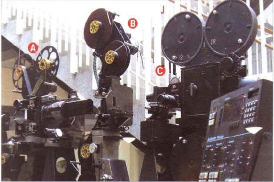
Figure 7.1. The optical printer used for Star Wars (1977). Projector A projected source footage. Projector B, which lacked a lens and lamp, held matte footage created through rotoscoping. Camera C exposed new film stock, but only in the region of the frame permitted by Projector B's footage. The white section of the matte footage, once processed, became transparent, while the black section became opaque. (Image courtesy of Industrial Light & Magic)
Rotoscoping has survived into the digital age and continues to be applied through compositing software and stand-alone programs. Rotoscoping, as used for digital compositing, is often referred to as roto.
The most difficult aspect of digital rotoscoping is the creation of accurate mask shapes. Although different programs, tools, and plug-ins exist to make the process easier, you must nevertheless decide where to keyframe the mask. You can key every single frame of the animation, but it is generally more efficient to key specific frames while letting the program interpolate the mask shape for the remaining, unkeyed frames. As such, there are two approaches you can take to plan the keyframe locations: bisecting and key poses.
The process of bisectin, as applied to rotoscoping, splits the timeline into halves. For example, you can follow these basic steps:
Move to frame 1, create a mask path, and set a key for the mask shape.
Move to the last frame of the sequence. Change the path shape to match the footage and set a new key.
Move to the frame halfway between frame 1 and the last frame. Change the mask shape and set a new key.
Continue the process of moving to a frame halfway between previous keyframes.
When you approach the keyframing in such a manner, fewer adjustments of the vertex positions are necessary than if the mask was shaped one frame at a time. That is, instead of keying at frames 1, 2, 3, 4, 5, 6, and so forth, key at frames 1, 60, 30, 15, 45, and so on.
Key pose, as used in the world of traditional animation, are the critical character poses needed to communicate an action or tell a story. If an animator is working pose-to-pose, they will draw the key poses before moving on to in-between drawings, or inbetweens. For example, if an animation shows a character lifting a box, the key poses include the character's start position, the character bent down touching the box, and the character's end position with the box lifted into the air.
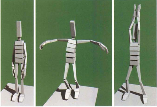
To simplify the rotoscoping process, you can identify key poses within a piece of footage. Once the poses are identified, shape the mask to fit the key poses and key the mask path. Because key poses usually involve an extreme, less-critical frames are left to interpolation by the program. An extreme is a pose that shows the maximum extension of appendages or other character body parts. For example, if an actor is doing jumping jacks, one extreme would show the character in a start position (see Figure 7.2). A second extreme would show the character jumping with his arms stretched out to the side. A third extreme would show the character's hands touching with his arms over his head. Once you have shaped and keyed the mask to fit all the key poses, you can shape and key the mask to fit the most critical inbetween poses.
Motion tracking, which tracks the position of a feature within live-action footage, falls into four main categories:
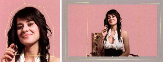
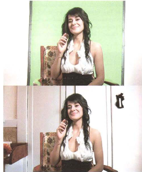
Transform Tracking if the live-action camera is static, this type of motion tracking is relatively simple. Unique features within the footage, sometimes as small as several pixels, are tracked so that composited elements can inherent the motion identified by the tracking. For example, you might motion track an actor's hand so that you can place a CG prop behind the fingers (see Figure 7.3). A similar but more complex challenge might involve tracking a CG head over the head of an actor in a scene. If the live-action camera is in motion, the tracking becomes more complex. If the camera's motion is significant and occurs along multiple axes, then matchmoving becomes necessary.
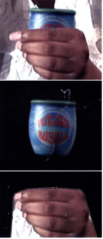
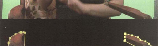
Figure 7.3. (Top) Detail of video composite with CG jar tracked to the hand of an actress (Center) Isolated jar layer. The jar's motion path, derived through transform tracking, is visible as the white line. (Bottom) Rotoscoped hand, which is placed back on top of the tracked jar. The yellow path is a mask.
Matchmoving With this form of motion tracking, you can replicate the complex movement of a live-action camera so that elements can be composited into the scene with proper position, translation, rotation, scale, and lens distortion. For instance, handheld or Steadicam camera work would generally require matchmoving as the camera is rotating and translating in all three axes and thus shifting the perspective of objects in the scene. (Note that matchmoving is often used as a generic term to cover all types of motion tracking.)
Plate Stabilization Through the process of plate stabilization, motion tracking data is used to remove jitter and other 2D camera shakes and motions.
Hand Tracking Hand tracking refers to transform tracking or matchmoving that is beyond the automated capabilities of motion tracking tools. If the hand tracking involves transform tracking, a 3D prop is keyframe animated so that its position lines up with a point appearing in imported footage. If the hand tracking involves matchmoving, a 3D camera is keyframe animated so that a virtual set lines up to the imported footage. (For more information on 3D cameras, as they apply to After Effects and Nuke, see Chapter 11, "Working with 2.5D and 3D.")
Masking and rotoscoping in After Effects and Nuke is carried out through various tools designed to create animatable spline paths. Motion tracking, on the other hand, is created through specific tracking effects and nodes.
The Pen tool supplies the primary means by which to create a mask in After Effects. However, Auto-trace and AutoBezier functions present alternative approaches. Motion tracking is carried out through the Track Motion tool.
In After Effects, all masks are dependent on a path. A path is a Bezier spline that indicates the area that the mask occupies. The path includes a number of vertex points, which define the curvature of the Bezier.
To create a path with the Pen tool manually, follow these steps:
Select a layer through the layer outline of the Timeline panel. Select the Pen tool (see Figure 7.4). LMB+click in the viewer of the Composition panel. Each click places a vertex point.
To close the path, LMB+click on or near the first vertex. The mouse pointer must be close enough to change to a close-path icon (a small pen icon with a circle beside it). Once the path is closed, any area outside the mask is assigned an alpha value of 0 and thus becomes transparent.
To end the path without closing it, choose the Selection tool. A nonclosed path will not function as a mask. However, you can close the path at a later time by selecting the path in the viewer and choosing Layer → Mask And Shape Path → Closed.
By default, the segments between each vertex of a mask path are linear. The vertex points themselves are considered corner points. However, smooth points are also available. A smooth point carries a direction handle and produces curved segments. To draw a smooth point, LMB+drag during the path-drawing process. That is, LMB+click where you want the vertex; without releasing the mouse button, continue to drag the mouse. The direction handle extends itself from the vertex point. The direction handle length, which affects the curvature of surrounding segments, is set once you release the mouse button. (Direction handles is Adobe's name for tangent handles.)
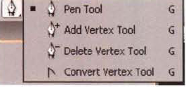
You can convert a corner point to a smooth point by selecting the Convert Vertex tool and LMB+clicking the vertex point in the viewer. Once the point is converted, a direction handle appears. You can move each side of the direction handle separately by LMB+dragging with the Convert Vertex tool or the Selection tool (see Figure 7.5). To return a smooth point to a corner point, LMB+click the point a second time with the Convert Vertex tool. You can delete a vertex point with the Delete Vertex tool. To insert a new vertex point into a preexisting path, choose the Add Vertex tool and LMB+click on the path at the position where you want the new vertex to appear.

Figure 7.5. (Top) Detail of mask path drawn with the Pen tool. Default linear segments span the vertex points. Selected vertex points are solid. The large hollow point at the top represents the first vertex drawn. (Bottom) Detail of mask with smooth points and curved segments. The selected vertex point is solid and displays its direction handle.
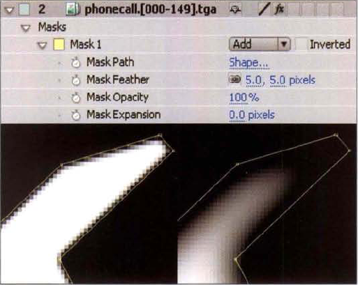
As soon as a mask is drawn, a Masks section is added for the corresponding layer in the layer outline (see Figure 7.6). A subsection is named after the new mask, such as Mask 1. The subsection includes Mask Opacity, Mask Feather, and Mask Expansion. Mask Opacity controls the alpha value of pixels within the mask. For example, a value of 50% assigns an alpha value of 0.5 on a 0 to 1.0 scale. Mask Opacity does not affect the alpha value of pixels that lie outside the mask. Mask Feather, on the other hand, introduces falloff to the alpha values at the edge of the mask. A value of 10, for example, tapers the alpha values from 1.0 to 0 over the distance of 10 pixels. Note that the mask is eroded inward when Mask Feather is raised above 0. In contrast, Mask Expansion expands the mask effect (if positive) or shrinks the effect (if negative). Both Mask Feather and Mask Expansion carry X and Y direction cells, which can be adjusted individually.
To select a mask vertex, LMB+click with the Selection tool. To select multiple vertices, select the mask name in the layer outline and then LMB+drag a selection marquee around the vertices you wish to choose. Direction handles are displayed only for selected vertices and the vertices directly to each side of those selected (assuming that they have smooth points).
You can use the keyboard arrow keys to translate selected vertex points one pixel at a time. To translate all the vertices of a mask as a single unit, double-click the mask path in the viewer with the Selection tool. A rectangular path transform handle appears (see Figure 7.7). To translate the path, LMB+drag the handle. To scale the path, LMB+drag one of the handles' corner points. To rotate the path, place the mouse pointer close to a handle corner; when the rotate icon appears, LMB+drag.

You can delete a mask at any time by selecting the mask name in the layer outline and pressing the Delete key. To hide the mask paths in the viewer temporarily, toggle off the Mask And Shape Path Visibility button at the bottom of the Composition panel (see Chapter 1).
You can animate the shape of a mask by toggling on the Stopwatch button beside the Mask Path property in the Masks section of the layer. Once the Stopwatch button is toggled on, you can LMB+drag one or more path vertex points in the viewer, which forces the current shape (and all the current point positions) of the path to be keyframed.
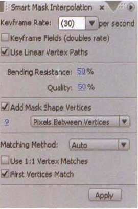
You can use the Smart Mask Interpolation tool to refine the way in which the program interpolates mask vertex positions between keyframes. To reveal the tool's controls, choose Window → Smart Mask Interpolation. The Smart Mask Interpolation panel opens at the bottom right of the After Effects workspace (see Figure 7.8).
To apply the tool, follow these steps:
Select two or more adjacent keyframes of a mask within the Timeline panel.
Set the options within the Smart Mask Interpolation panel.
Click the Apply button. The tool places new keyframes between the selected keyframes.
The following suggestions are recommended when setting the tool's options:
If you do not want a new keyframe at every frame of the timeline, reduce the Keyframe Rate value. For example, if the project frame rate is 30 and Keyframe Rate is set to 10, ten keyframes are added per second with a gap of two keyframes between each one. (Additionally, the tool always adds a keyframe directly after the first keyframe selected and directly before the last keyframe selected.)
Deselect Use Linear Vertex Paths. This forces the vertex motion paths to remain smooth.
If the mask shape does not undergo a significant shift in shape between the selected keyframes, set Bending Resistance to a low value. This ensures that relative distance between vertex positions is maintained-that is, the path bends more than it stretches. If the mask shape undergoes a significant change in shape, set Bending Resistance to a high value. A high value allows the vertices to drift apart and the mask shape to stretch.
If you do not want the tool to add additional vertices, deselect the Add Mask Shape Vertices check box. That said, complex interpolations are generally more successful if vertices are added.
Leave Matching Method set to Auto. Otherwise, the tool may change each vertex type from linear to smooth or vice versa.
Keep in mind that Smart Mask Interpolation tool is purely optional. Nevertheless, it offers a means to set a series of keyframes automatically. In addition, it can produce a mask interpolation different from the interpolation the program normally creates between pre-existing keyframes.
You can draw multiple masks for any layer. Each new mask is consecutively numbered (Mask 1, Mask 2, and so on). If more than one mask exists for a layer, it's important to choose a mask mode (blending mode) for each mask. You can find the mask modes menu beside the mask name in the layer outline (see Figure 7.6 earlier in this chapter). Here's how each mode functions:
None disables the mask.
Add adds the mask to the mask above it. If there is only one mask for the layer, Add serves as an on switch.
Subtract subtracts the mask from the mask above it (see Figure 7.9).
Intersect adds the mask to the mask above it but only for the pixels where the masks overlap. The masks are made transparent where they do not overlap (see Figure 7.9).
Lighten adds the mask to the mask above it. However, where masks overlap, the highest Mask Opacity value of the two masks is used.
Darken adds the mask to the mask above it. However, where masks overlap, the lowest Mask Opacity value of the two masks is used.
Difference adds the mask with the mask above it. However, where masks overlap, the lower mask is subtracted from the upper mask (see Figure 7.9).
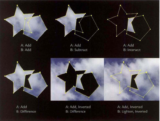
To invert the result of any mask, select the Inverted check box beside the mask name in the layer outline. The mask blend modes take into account Mask Opacity values for the masks assigned to a layer. For example, if Mask A is set to Add and has a Mask Opacity of 100% and Mask B is set to Subtract with a Mask Opacity of 50%, the area in which the masks overlap receives an opacity of 50%. That is, 50% is subtracted from 100%.
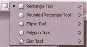
After Effects offers several ready-made mask shapes. To apply one, select a layer in the layer outline, select a shape tool (see Figure 7.10), and LMB+drag in the viewer. Once the mouse button is released, the size of the shape path is set. Nevertheless, using the Selection tool, you can manipulate any of the resulting vertex points as you would a hand-drawn path. The resulting path is added to the Masks section in the layer outline and receives a standard name, such as Mask 3.
If a layer is not selected when a shape tool is applied, the shape becomes a separate shape layer and does not function as a mask. However, you can convert a shape to a mask path by employing the Auto-trace tool (see the next section).
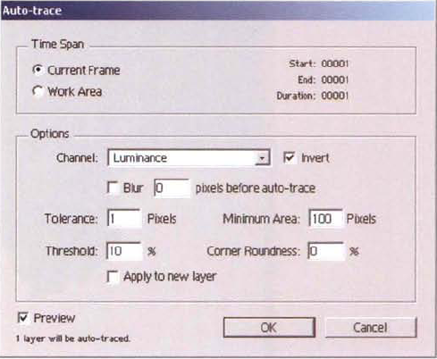
The Auto-trace tool automatically creates a mask based on the RGB, alpha, or luminance values within a layer. To apply it, follow these steps:
Select the layer that you want to trace. Choose Layer → Auto-trace. The Auto-trace dialog box opens (see Figure 7.11). The selected layer becomes the input layer.
Change the Channel menu to Red, Green, Blue, Alpha, or Luminance to determine how the tool will generate the mask path or paths. Select the Preview check box to see the result of the tool. One or more mask paths are automatically drawn along high-contrast edges.
Adjust the dialog box properties to refine the paths (see the list after this set of steps).
Deselect the Apply To New Layer check box. Click the OK button to close the dialog box. The new path (or paths) is added to the input layer (see Figure 7.12). By default, the mask blend mode menu (beside the mask name in the layer outline) is set to None. To see the resulting matte in the alpha channel, change the menu to Add.
The Auto-trace tool is best suited for fairly simple layers that contain a minimal number of high-contrast edges. Nevertheless, the Auto-trace dialog box contains several properties with which to adjust the results:
Current Frame, if selected, creates paths for the current timeline frame.
Work Area, if selected, creates paths for every frame of the timeline work area. The vertex positions are automatically keyframed over time.
Invert, if selected, inverts the input layer before detecting edges.
Blur, if selected, blurs the input layer before detecting edges. This reduces the amount of noise and minimizes the number of small, isolated paths. The Pixels Before Auto-Trace cell sets the size of the blur kernel and the strength of the blur.
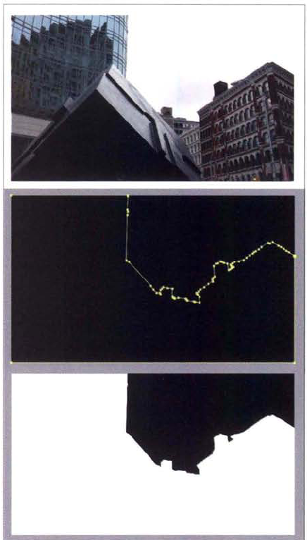
Figure 7.12. (Top) Photo of city used as input layer (Center) Auto-traced mask with Channel set to Luminance, Tolerance set to 1, Threshold set to 10%, Minimum Area set to 100 pixels, Corner Roundness set to 0, and Invert selected (Bottom) Resulting alpha channel. A sample After Effects project is included as
autotrace.aepin the Tutorials folder on the DVD.Threshold sets the sensitivity of the edge detection. Input pixel values above the Threshold value earn an alpha value of 1.0; input pixels below the Threshold value earn an alpha value of 0. Paths are drawn at the borders between resulting sets of pixels with 0 and 1.0 alpha values. The Threshold cell operates as a percentage; nevertheless, this is equivalent to a 0 to 1.0 scale where 50% is the same as 0.5.
Minimum Area specifies the pixel area of the smallest high-contrast feature that will be traced. For example, a value of 25 removes any path that would normally surround a high-contrast dot that is less than 5×5 pixels in size.
Tolerance sets the distance, in pixels, a path may deviate from the detected edges. This is necessary to round the path at vertex positions when using the Corner Roundness property. The higher the Corner Roundness value, the smoother and more simplified the paths become.
Apply To New Layer, if selected, places the paths on a new Auto-trace layer. The Auto-trace layer is solid white; the result is a white shape cut out by the new masks.
You can use any closed path to rotoscope in After Effects. Once the Stopwatch button beside the Mask Path property is toggled on, you can reposition the vertices over time and thus allow the program to automatically place keyframes for the mask shape.
At the same time, you can convert any preexisting path to a RotoBezier path to make the rotoscoping process somewhat easier. To do so, select a mask name in the layer outline and choose Layer → Mask And Shape Path → RotoBezier. RotoBezier paths differ from manually drawn paths in that they do not employ direction handles. Instead, each RotoBezier vertex uses a tension value that affects the curvature of the surrounding segments (see Figure 7.13). You can adjust the tension value by selecting a vertex with the Convert Vertex tool and LMB+dragging left or right in the viewer. LMB+dragging left causes surrounding segments to become more linear. LMB+dragging right causes the segments to gain additional curvature.

Figure 7.13. (Left) Mask path with default linear segments (Center) Mask path converted to smooth points with direction handles visible (Right) Mask path converted to RotoBezier
You can adjust the direction handles of a path with smooth points and thus match any shape that a RotoBezier path may form. However, such adjustments are considerably more time intensive than manipulating the RotoBezier tension weights. Hence, RotoBezier paths tend to be more efficient during the rotoscoping process. Nevertheless, if a required mask needs numerous sharp corners, it may be more practical to stick with a manually drawn path that has default corner points.
After Effects comes equipped with a built-in motion tracker, which is called Track Motion or Stabilize Motion, depending on the settings. To apply Track Motion, follow these steps:
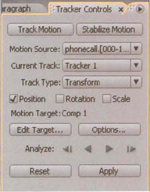
Select the layer you wish to track in the layer outline. Choose Animation → Track Motion. A Tracker Controls panel opens at the bottom right of the After Effects workspace (see Figure 7.14). In addition, the layer is opened in the Layer panel.
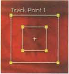
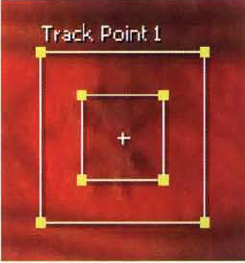
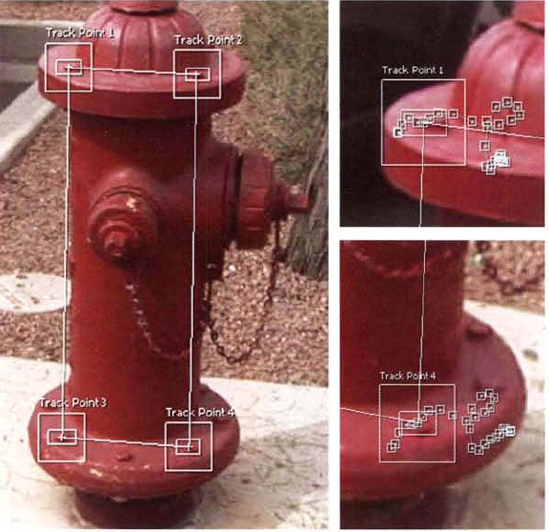
A single track point, Track Point 1, is supplied and is placed in the viewer of the Layer panel (see Figure 7.15). The inner box establishes the feature region, which the tracker attempts to follow across multiple frames. For successful tracking, the feature should be an identifiable element, such as the iris of an eye, which is visible throughout the duration of the timeline. The outer box establishes the search region, in which the tracker attempts to locate the feature as it moves across multiple frames. The center + sign is the attach point, which is an X, Y coordinate to which a target layer is attached. The target layer receives the tracking data once the tracking has been completed. You can choose the target layer by clicking the Edit Target button in the Tracker Controls panel and choosing a layer name from the Layer menu of the Motion Target dialog box.
Position Track Point 1 over an identifiable feature. Scrub through the timeline to make sure the feature you choose is visible throughout the duration of the footage. The smaller and more clearly defined the selected feature, the more likely the tracking will be successful. You can adjust the size of the region boxes to change the tracker sensitivity; LMB+drag one of the region box corners to do so.
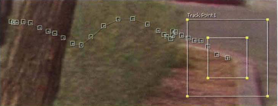
To activate the tracker, return the timeline to frame 1 and press the Analyze Forward play button in the Tracker Controls panel. The tracker advances through the footage, one frame at a time, and creates a motion path for Track Point 1 (see Figure 7.16). The motion path includes keyframe markers, in the form of hollow points, for each frame included in the tracking.
Scrub through the timeline. If Track Point 1 successfully follows the feature selected in step 3, you can transfer the data to the target layer. To do this, click the Apply button in the Tracker Controls panel and press OK in the Motion Tracker Apply Options dialog box. Keyframes are laid down for the target layer's Position property. The target layer thus inherits the motion identified by the tracker. Note that the view automatically changes to the viewer of the Composition panel when the Apply button is pressed.
If the motion to be tracked is complicated, you can add a second tracking point and corresponding icon by selecting the Rotation and/or Scale check boxes in the Tracker Controls panel. Track Point 2's icon is attached to the Track Point 1 icon in the viewer. However, you can adjust each icon separately. When you add a second point, the tracker is able to identify motion within footage that undergoes positional, rotational, and scale transformations (see Figure 7.17). If Position, Rotation, and Scale check boxes are selected, the target layer receives keyframes for the corresponding properties.

The Track Motion tool stores the position of the keyframe markers for the tracked layer as keyframes under a Motion Trackers section in the layer outline (see Figure 7.18). Each track point is given its own subsection. Within these subsections, the keyframes are divided between Feature Center, Confidence, and Attach Point properties. Feature Center stores the X and Y position of the Track Point icon. Attach Point stores the X and Y position of its namesake. By default, Feature Center and Attach Point values are identical. However, you can reposition the attach point + icon in the viewer before using the Analyze Forward button; this offsets the inherited motion of the target layer and creates unique values for the Attach Point property. If adjusting the attach point + icon proves inaccurate, you can enter new values into the Attach Point Offset property cells after the keyframes are laid down in the Motion Trackers section. For example, entering −100, 0 causes the target layer to move 100 pixels further to the left once the Apply button in the Tracker Controls panel is clicked.
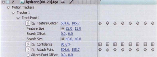
The Confidence property represents the motion tracker's estimated accuracy. With each frame, the tracker reports a Confidence value between 0% and 100%. If Track Point 1 suddenly loses its selected feature and goes astray, the Confidence value drops. This is an estimated accuracy, however. The value may stay relatively high even if Track Point 1 jumps to a completely inappropriate part of the frame. Nevertheless, you can use the Confidence to drive the action of the tracker. To do so, click the Options button in the Tracker Controls panel. In the Motion Tracker Options dialog box (Figure 7.19), you can choose a Confidence threshold by changing the % cell in the lower-right corner. You can choose an action for the tracker if it drops below the threshold by changing the If Confidence Is Below menu. The Continue Tracking option is the default behavior, which may allow the track points to run astray. The Stop Tracking option stops the tracker when the Confidence level drops too low. This gives the user a chance to adjust the track point positions before applying the Analyze Forward or Analyze Backward buttons again. The Extrapolate Motion option attempts to relocate the selected feature if the Confidence level drops too low. The Adapt Feature option forces the tracker to identify a new pattern within the search region, which means that the feature identified for the first frame is no longer used.
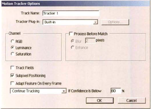
In addition to the Confidence settings, several other options provide flexibility. Through the Channel section, you can switch the tracker to Luminance, RGB, or Saturation examination. If you select the Process Before Match check box, you can force the tracker to blur or enhance (edge sharpen) the image before tracking. Blurring the image slightly may help remove interference created by film or video grain. Enhancing may aid the tracker when there is significant motion blur. The strength of the blur or enhance is set by the Pixels cell. Subpixel Positioning, when selected, allows track point position values to be stored with decimal values. If Subpixel Positioning is unselected, the positions are stored as whole pixel numbers. With low-resolution material, Subpixel Positioning may help perceived accuracy.
Aside from adjusting the properties within the Motion Tracker Options dialog box, you can apply the following techniques if the tracking proves to be inaccurate:
Move to the frame where a track point has "lost sight" of its chosen feature. Manually position the track point icon so that it is centered over the selected feature once again. Press the Analyze Forward button again. New keyframes are laid over old keyframes.
If the problem area is only a few frames in duration, manually step through with the Analyze 1 Frame Forward or Analyze 1 Frame Backward button.
If a track point slips away from its feature, LMB+drag the corresponding keyframe marker to an appropriate position within the viewer. The keyframes in the Timeline panel are automatically updated.
Adjust the errant track point's search and feature regions. If the feature region is too small, the track point may suddenly lose the feature. If the search region is too large, the track point may be confused by similar patterns that lie nearby.
Edit the keyframes in the Timeline panel using standard editing tools, such as the Graph Editor or Keyframe Interpolation. You can delete keyframes to remove "kinks" in the track point motion path.
If you decide to return to the Motion Tracker after working with other tools, change the Motion Source menu in the Tracker Controls panel to the layer that carries the tracking information.
By default, the Track Motion tool operates as a transform tracker. However, you can change the functionality by switching the Track Type menu in the Tracker Controls panel to one of the following options:
Parallel Corner Pin tracks skew and rotation. It utilizes four track points (see Figure 7.20). You can adjust the position and size of the first three track points. Track Point 4, however, stays a fixed distance from Track Points 2 and 3 and cannot be manually positioned. Nevertheless, the Parallel Corner Pin tracker is ideal for tracking rectangular features shot with a moving camera. TV screens, billboards, and windows fall into this category. When the tracking data is applied, the target layer is given a specific Corner Pin transform section with keyframes matching each of the four points. In addition, the Position property is keyed.
Perspective Corner Pin tracks skew, rotation, and perspective changes. It utilizes four track points. Unlike with Parallel Corner Pin, however, all four point icons can be adjusted in the viewer. Perspective Corner Pin is ideal for tracking rectangular features that undergo perspective shift. For example, you can place a CG calendar on the back of a live-action door that opens during the shot. When the tracking data is applied, the target layer is given a Corner Pin transform section with keyframes matching each of the four points; in addition, the Position property is keyed. Perspective Corner Pin is demonstrated in "AE Tutorial 7: Corner Pin Tracking with a Non-Square Object" at the end of this chapter.
Raw operates as a transform tracker but does apply the tracking data to a target layer. Instead, the keyframes are stored by the layer's Feature Center, Confidence, and Attach Point properties. The Raw option is designed to provide keyframe data to expressions or operations where the copying and pasting of tracking data keyframes may prove useful.
Stabilize tracks position, rotation, and/or scale to compensate for (and thus remove) camera movement within the layer. If the Rotation and/or Scale check boxes are selected, two tracker points are provided. In contrast to Transform mode, the tracking data is applied to the layer that is tracked and there is no target layer. As such, the layer's Anchor Point, Position, Scale, and Rotation properties are keyframed.

You can create a mask in Nuke by connecting the output of a node to a second node's Mask input. You can also create a mask with the Bezier node, which is automatically keyframed in anticipation of rotoscoping. The Tracker node, in contrast, can track motion with one, two, three, or four track points.
Numerous Nuke nodes, including filter nodes and merge nodes, carry a Mask input. This is symbolized by an arrow stub appearing on the right side of a node. You can LMB+drag the arrow stub and thereby extend the pipe to another node (see Figure 7.21). Once the Mask input is connected, the Mask check box is selected automatically in the masked node's properties panel. By default, the Mask menu is set to Rgb.alpha, which means that the mask values are derived from the input node's alpha. However, you can change the Mask menu to Rgb. channel, Depth.Z, or other specialized channel.
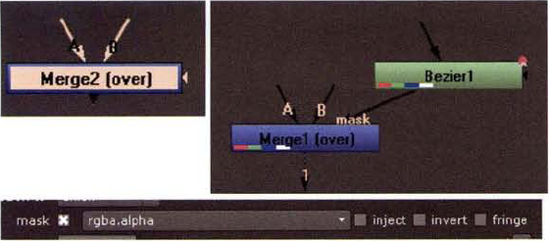
Figure 7.21. (Top Left) Merge node's Mask input arrow stub, seen on the right side of the node icon (Top Right) Merge node's Mask input pipe connected to the output of a Bezier node (Bottom) Merge node's Mask parameter with Inject, Invert, and Fringe check boxes
Here are a few example connections that take advantage of the Mask input:
A Read node, which carries a black-and-white bitmap of text, is connected to the Mask input of a Defocus node. Thus the blur appears only where the bitmap is white (see Figure 7.22). With this example, the Defocus node's Mask parameter is set to Rgb.red. Again, the Mask parameter determines which Mask input channel contributes values to the alpha matte. Rgb.green or Rgb.blue would work equally well in this situation.
A Ramp node is connected to the Mask input of a Merge node. Thus the Merge node's input A wins out where the ramp is white (see Figure 7.22). The Merge node's input B wins out where the ramp is black. (This assumes that input A and input B possess solid-white alpha channels.) With this example, the Merge node's Mask parameter is set to Rgb.alpha (the Ramp node pattern appears in the RGB and alpha channels).
A Bezier node is connected to the Mask input of a Merge node, thus determining which portion of the Merge node's input A is used. For a demonstration of this technique, see the next section plus the section "Nuke Tutorial 3 Revisited: Finalizing the Composite" at the end of this chapter.
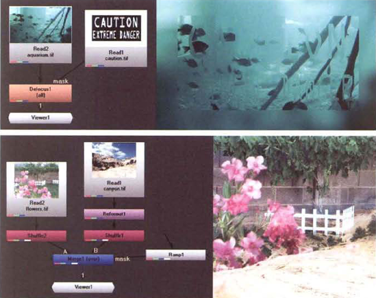
Figure 7.22. (Top Left) The output of a Read node is connected to the Mask input of a Defocus node. (Top Right) The resulting blur is contained to parts of the Read node's bitmap that are white. A sample Nuke script is included as filter_mask.nk in the Tutorials folder. (Bottom Left) The output of a Ramp node is connected to the Mask input of a Merge node. (Bottom Right) The resulting merge fades between input A and input B. A sample Nuke script is included as ramp_mask.nk in the Tutorials folder on the DVD.
Perhaps the easiest way to create a mask is to use a Bezier node. To apply a Bezier, you can follow these steps:
In the Node Graph, RMB+click and choose Draw → Bezier. Open the new Bezier node's properties panel.
In the viewer, Ctrl+Alt+click to place a vertex. Continue to Crtl+Alt+click to place additional vertices. By default, the Bezier path is closed.
You can edit the Bezier path at any point as long as the Bezier node's properties panel is open. To move one vertex, LMB+drag the vertex point. To move multiple vertices, LMB+drag a selection marquee around the points and use the central transform handle for manipulation. To move a tangent handle, LMB+drag one of the two handle points. To insert a new vertex, Ctrl+Alt+click on the path. To delete a vertex, select it in the viewer and press the Delete key.
The path tangents are smooth by default (see Figure 7.23). However, you can convert a tangent by RMB+clicking over the corresponding point and choosing Break or Cusp from the menu. Cusp forces linear segments to surround the vertex and is therefore appropriate for making sharp corners on the path. Break splits the tangent handle so that the two ends can be moved independently. You can affect the curvature of the corresponding path segment by LMB+dragging the tangent handle to make it shorter or longer.
By default, the pixels within the closed path receive an alpha value of 1.0, while the pixels outside the path receive an alpha value of 0. However, you can reduce the Bezier node's Opacity slider and thus lower the alpha value within the path. To feather the edge of the resulting alpha matte, do one of the following:
Adjust the Extra Blur slider of the Bezier node. Positive values feather the edge outward. Negative numbers feather the edge inward. To soften the resulting edge even further, lower the Falloff parameter below 1.0.

Figure 7.23. A Bezier path with selected vertices. Cusp vertices are identifiable by their lack of tangent handles. Break tangents possess left and right tangent handles that can be rotated individually. Smooth vertices feature tangent handles that are fixed in a straight line. The transform handle is the central circle.
Ctrl+LMB+drag a vertex in the viewer. By holding down the Ctrl key, you can create a duplicate vertex point. When you release the mouse key, the edge is feathered from the original vertex position to the position of the duplicate vertex. To delete the duplicated vertex and remove the feather, RMB+click over the duplicate vertex and choose Unblur.
In the viewer, RMB+click over a vertex and choose Blur. A duplicate vertex is created and is slightly offset from the original vertex.
A Bezier node can only support a single path. However, you can combine the results of two or more Bezier nodes with one of the following techniques:
Connect the output of the one Bezier node to the input of another Bezier node. The paths are added together and the output alpha channel is identical to the RGB (see Figure 7.24).
Connect each Bezier output to a Merge node with default settings. The result is the same as connecting the Beziers directly to each other. You can continue to connect additional Bezier nodes through the A2, A3, and A4 inputs.
To use Merge nodes with nondefault Operation menu settings, connect the Bezier nodes in pairs (see Figure 7.24). For example, to subtract the Bezier connected to the Merge node's input B from the Bezier connected to Merge node's input A, set the Operation menu to Minus.
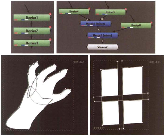
Figure 7.24. (Top Left) Three Bezier nodes connected in a series (Top Right) Three Bezier nodes connected in pairs to two Merge nodes (Bottom Left) Result of Bezier nodes connected in a series (Bottom Right) Result of Bezier nodes connected to Merge nodes with the Operation menus set to Minus. A sample Nuke script is included as three_beziers.nk in the Tutorials folder on the DVD.
The Bezier node is designed for animation. When the Bezier is drawn, the shape of its path is automatically keyed for the current frame of the timeline. The keyframe is indicated by the cyan shading of the Shape parameter of the Bezier node's properties panel (see Figure 7.25). The Shape parameter is represented by two cells. The leftmost cell indicates the shape number. The second cell indicates the total number of shapes. If you move the timeline to a different frame and adjust the path, the shape is automatically keyframed, the shape is assigned a new number, and the total number of shapes increases by 1. Once multiple shapes exist, Nuke morphs between shapes. The morph is based on a spline interpolation between vertex points. You can force the interpolation to be linear, however, by selecting the Linear Interpolate check box.
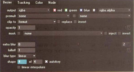
Figure 7.25. The properties panel of a Bezier node. The Bezier has four shapes that have been keyed.
You can alter the nature of the shape morph by changing the Shape bias slider, which is found to the right of the Shape cells. If you LMB+click and drag the slider, the interpolation updates the path in the viewer. If you move the slider toward 1.0, the interpolation is biased toward the keyframed shape with the higher frame number. If you move the slider toward −1, the interpolation is biased toward the keyframed shape with the lower frame number. Note that the slider returns to 0 when the mouse button is released and the resulting shape is automatically keyframed. You can revise a keyframe at any time by moving the timeline to the keyed frame and either moving vertex points in the viewer or adjusting the Shape bias slider.
Nuke provides a Tracker node (in the Transform menu). The node offers five main modes, each of which can be set by changing the Transform menu in the Transform tab of its properties panel. The modes follow:
None is the mandatory mode when calculating the motion track. It operates in the same manner as the Match-Move mode but does not apply the transforms to the connected input. (See the next section for more information.)
Match-Move serves as a transform tracker and is designed to match the movement detected through the motion tracking process.
Stabilize removes 2D camera movement by neutralizing the motion detected through the tracking process. Selected features are pinned to points within the frame without concern for where the edge of the frame may wind up.
Remove Jitter removes 2D camera movement but only concerns itself with high-contrast movement. The mode does not attempt to pin selected features to specific points within the frame. In the other words, Remove Jitter neutralizes small-frequency noise, such as camera shake, without disturbing large-frequency noise, such as a slow camera pan or slow handheld drift.
Add Jitter allows you to transfer the camera motion from a piece of footage to an otherwise static node.
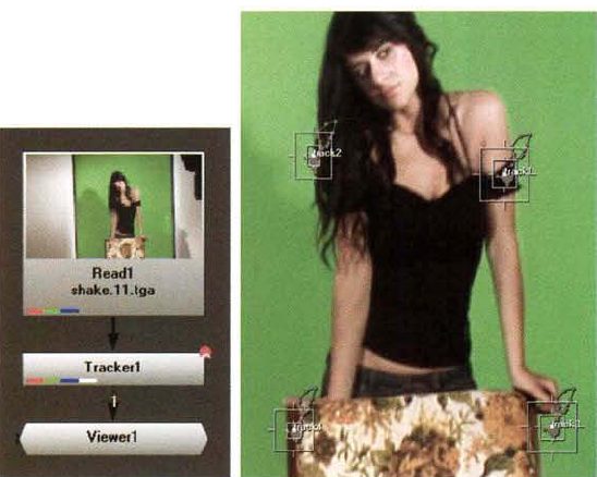
By default, the Transform menu of the Tracker node is set to None. It is therefore ready to calculate the motion track with one to four track anchors (tracking points). By default, one track anchor, Tracker 1, is activated. Each track anchor is represented in the viewer by a double-box icon and is named Trackn (see Figure 7.26). The inner box establishes the pattern area, which the tracker attempts to follow across multiple frames. For successful tracking, the pattern should be an identifiable element, such as the iris of an eye, that is visible throughout the duration of the timeline. The outer box establishes the search area in which the tracker attempts to locate the pattern as it moves across multiple frames.

Figure 7.26. (Left) Tracker 1 anchor with a motion path (Right) The Tracker tab of the Tracker node's properties panel
To activate additional track anchors, select the Tracker 2, Tracker 3, and/or Tracker 4 Enable check boxes in the Tracker tab of the Tracker node's properties panel (see Figure 7.26). Each track anchor has the ability to track translation, rotation, and scale. You can activate this ability by selecting the T, R, or S check box beside each track anchor name in the Tracker tab. You can position a track anchor by LMB+dragging its center point in the viewer. You can adjust the size of the inner or outer box by LMB+dragging one of its boundaries (edges).
Once the anchors are positioned, you can calculate the motion tracks by using the track play buttons in the Tracker tab. The buttons offer a means to track forward, backward, one frame at a time, or through a defined frame range. You can apply the track play buttons multiple times and thus overwrite preexisting tracking data. Once tracking data exists, each anchor is given a motion path in the viewer (see Figure 7.26). Points along the paths represent the location of an anchor for any given frame. You can interactively move a point for the current frame by LMB+dragging the matching anchor.
Once motion tracks exist, you can utilize the tracking data. If you are transform tracking (which Nuke calls match-moving) or adding jitter, you can disconnect the Tracker node from the tracked source and reconnect it to the output of the node to which you want to apply the tracking data. You can also duplicate the Tracker node and connect the duplicated node to the output of the node to which you want to apply the tracking data. If you are stabilizing the footage or removing jitter, the Tracker node can stay in its current position within the node network. In any of these situations, the Transform menu must be set to the appropriate mode. The workflows for each of these scenarios are detailed in the following sections.
To use the Tracker node in the Match-Move mode, you can follow these basic steps:
Select the node that you wish to track. For instance, select a Read node that carries video footage. RMB+click and choose Transform → Tracker.
In the Settings tab, set the Warp Type menu to an appropriate transformation set. If the footage you are tracking has a static camera or a camera that has no significant pan or tilt, set the menu to Translate. If the camera does go through a sizable pan or tilt, set the menu to Translate/Rotate. If the camera zooms, set the menu to Translate/Rotate/Scale. If the feature or pattern you plan to track goes through any type of rotation or moves closer to or farther from the camera, set the menu to Translate/Rotate/Scale (even if the camera is static).
In the Tracker tab, select the Tracker 1 T, R, and S check boxes to match the Warp Type menu. For instance, if Warp Type is set to Translate/Rotate, then select the T and R check boxes (see Figure 7.26). It may be possible to undertake the tracking with one track anchor. However, this is dependent on the complexity of the footage. You can start with one track anchor and, if the tracking fails or is inaccurate, add additional track anchors by selecting their Enable check box and matching T, R, and/or S check boxes.
Position the anchor or anchors using the suggestions in the previous section. Calculate the tracks by using the track play controls in the Tracker tab, which include a means to play forward to the end, play backward to the beginning, or step one frame at a time in either direction. To refine the results, readjust the anchor positions and anchor regions and use the track play buttons multiple times.
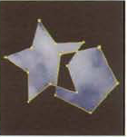
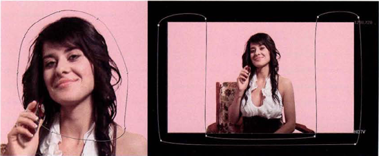
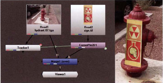
Once you're satisfied with the tracking results and have motion paths that run the complete duration of the timeline, select the Tracker node and choose Edit → Duplicate. Connect the duplicated Tracker node to the output of the node to which you wish to apply the motion. For instance, connect the Tracker node to a Read node that carries a CG render of a prop or a static piece of digital art. Open the duplicated Tracker node's properties panel. Switch to the Transform tab and change the Transform menu to Match-Move. (If the menu is left set to None, the tracking data is not used.) For example, in Figure 7.27, a starburst graphic is transform-tracked to the shoulder of a model. Because the camera zooms in and is shaky, three track anchors are used. A duplicate of the Tracker node (Tracker2) feeds the tracking data to the Read2 node, which carries the graphic. To offset the graphic so that it rests on a desirable portion of the shoulder, a Transform node is added between the Read2 node and the Tracker2 node. The graphic and the original video footage are combined with a Merge node.
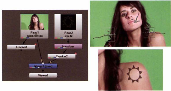
Figure 7.27. (Left) Transform tracking network. A starburst graphic is transform tracked to the shoulder of a model. (Top Right) The three track anchors used by the Tracker1 node. The Tracker2 node is a duplicate of the Tracker1 node and has its Transform menu set to Match-Move. (Bottom) A detail of the starburst merged with the footage after the tracking data is applied. A sample Nuke script is included as
transform_track.nkin the Tutorials folder on the DVD.
It's not unusual for the Track To The First Frame or Track To The Last Frame buttons to suddenly stop midway through the footage. This is due to an anchor "losing sight" of a selected pattern. This may be caused by a sudden camera movement, heavy motion blur, or a significant change in perspective, deformation, or lighting. Heavy film or video grain can also interfere with the process. When this occurs, there are several approaches you can try:
With the timeline on the frame where the tracker has stopped, reposition the anchor that has gone astray. Press the track play buttons again.
Move ahead on the timeline by several frames. Position all the anchors so that they are centered over their selected patterns. Press the track play buttons again. If the tracking is successful, there will be gaps in the corresponding curves where no keyframes are placed. You can edit the gaps in the Curve Editor.
If the problem area is only a few frames in duration, manually step through with the Track To The Previous Frame or Track To The Next Frame buttons. If an anchor slips away from its pattern, manually reposition it in the viewer.
Adjust the errant anchor's search and pattern boxes. If the pattern box is too small, the anchor may suddenly lose the pattern. If the search box is too large, the anchor may be confused by similar patterns that lie nearby.
Raise the Max_Error parameter value (found in the Settings tab of the Tracker node). This allows for a greater deviation in detection to exist. Although this may prevent the tracker from stopping, it may cause an anchor to jump to a neighboring pattern.
The Add Jitter mode uses the same workflow as the Match-Move mode. However, Match-Move is designed to add motion to an otherwise static element, which in turn is composited on top of the tracked footage. Add Jitter, in contrast, is suited for adding artificial camera movement to an otherwise static frame. For example, you can use a Tracker node to motion track the subtle camera shake of video footage, then use a duplicate of the Tracker node with the Transform menu set to Add Jitter to impart the same camera shake to a matte painting held by a Read node.
To use the Tracker node in the Stabilize mode, you can follow these basic steps:
Select the node that you wish to stabilize. RMB+click and choose Transform → Tracker. Open the Tracker node's properties panel. In the Settings tab, set the Warp Type menu to an appropriate transformation set. If the footage you are stabilizing has only a minor motion, such as a slight pan or down-to-up tilt, set the menu to Translate. If the camera has chaotic or aggressive motion, set the menu to Translate/Rotate. If the camera tilts side to side (as with a "Dutch" angle), set the menu to Translate/Rotate. If the camera zooms, set the menu to Translate/Rotate/Scale.
In the Tracker tab, select the Tracker 1 T, R, and S check boxes to match the Warp Type menu. For instance, if Warp Type is set to Translate/Rotate, then select the T and R check boxes. It may be possible to undertake the tracking with one track anchor. However, this is dependent on the complexity of the footage. You can start with one track anchor and, if the tracking fails or is inaccurate, add additional track anchors by selecting their Enable check box and matching T, R, and/or S check boxes.
Position the anchor or anchors using the section "Tracking with the Tracker Node" as a guide. Calculate the tracks by using the track play buttons in the Tracker tab. To refine the results, readjust the anchor positions and anchor regions and use the track play buttons multiple times. For problem-solving suggestions, see the previous section.
Once you're satisfied with the tracking results and have motion paths that run the complete duration of the timeline, change the Transform menu to Stabilize. The footage is automatically repositioned so that the selected patterns are fixed to points within the frame. For example, in Figure 7.28, an extremely shaky piece of footage is stabilized so that the model appears perfectly still.
The Remove Jitter mode uses the same workflow as the Stabilize mode. However, Remove Jitter makes no attempt to fix selected features to specific points within the frame. Instead, Remove Jitter neutralizes low-frequency noise without disturbing larger camera movements. To see the difference between the two modes, you can change the Transform menu from Remove Jitter to Stabilize or vice versa.
Nuke provides two additional nodes for applying motion tracking data: CornerPin2D and Stabilize2D. Both nodes require that you transfer data from a Tracker node through the process of linking.
CornerPin2D (Transform → CornerPin) is designed for corner pin tracking, whereby four anchors are used to define the corners of a rectangular feature that moves through a scene. In turn, the track data is used to translate, rotate, scale, and skew the output of a target node so that it fits over the rectangular feature. For example, corner pin tracking is necessary when replacing a TV screen with a video news broadcast that was shot at a different location. A CornerPin2D node is connected to the output of the target node. The output of the CornerPin2D node is then merged with the node that is tracked. The tracking data is transferred from the Tracking node through linking. To create a link, you can follow these steps:
Move the mouse pointer over the Animation button beside the Track1 X and Y cells in the Tracker tab of the Tracker node. Ctrl+LMB+drag from the Track1 Animation button to the To1 Animation button in the CornerPin2D tab of the CornerPin2D node. As you Ctrl+LMB+drag, the mouse icon changes and a small + sign appears. Once the mouse pointer reaches the To1 Animation button, release the mouse button. A link is created, the To1 cells turn gray blue (see Figure 7.29), and a green connection is drawn between the two nodes in the Node Graph.
Repeat the process of linking Track2 and To2, Track3 and To3, and Track4 and To4.
For additional details on the process, see the section "Nuke Tutorial 7: Corner Pin Tracking with a Non-Square Object" later in this chapter.
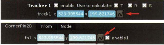
Figure 7.29. (Top) Track1 X and Y cells (Bottom) To1 X and Y cells after the link is established. Animation buttons are indicated by arrows.
Stablize2D (Transform → Stabilize) stabilizes an input through the use of two track points. The Track1 and Track2 parameters must be linked to the equivalent track points of a Tracker node. Since the result is likely to place the input outside the frame edge, Offset X and Y parameters are provided.
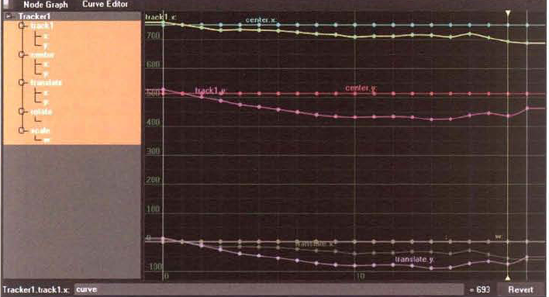
Once motion tracks are calculated, they are stored within the Tracker node. You can edit a motion track as a set of curves by clicking the Animation button beside the track name (such as Track1) in the Tracker tab and choosing Curve Editor from the menu. If the T, R, and S check boxes were selected before the calculation, the Curve Editor will display Trackn X, Trackn Y, Centern X, Centern Y, Translate X, Translate Y, Rotate, and Scale W curves (see Figure 7.30). If the Transform menu of the Tracker node is set to Stabilize, Match-Move, Remove Jitter, or Add Jitter, updates to the curves will instantly alter the appearance of the tracked footage or element in the viewer.
The type of tracking you are attempting determines which curves should be edited. Here are a few guidelines:
If you are transform tracking, edit the Center X and Center Y curves to offset the tracked element. Offsetting may be necessary when the track anchors are not positioned at the location where you wish to place the tracked element. Adjusting the Center X and Y curves may prevent the need for an additional Transform node, as is the case in the example given for Figure 7.27 earlier in this chapter.
If you are stabilizing a plate and there are minor flaws in the stabilization, it's best to refine the track anchor motion paths in the viewer interactively, but only after the Tracker node's Transform menu is temporarily set to None. Although you can alter the Trackn X and Trackn Y curves in the curve editor, it's difficult to anticipate the altered curves' impact on the stabilization.
If you are corner pin tracking, whereby the Tracker node is linked to a CornerPin node, edit the Trackn X and Trackn Y curves. There will be four sets of Trackn curves to edit (one for each anchor). Adjusting these curves allows you to fine-tune the perspective shift of the tracked rectangular element.
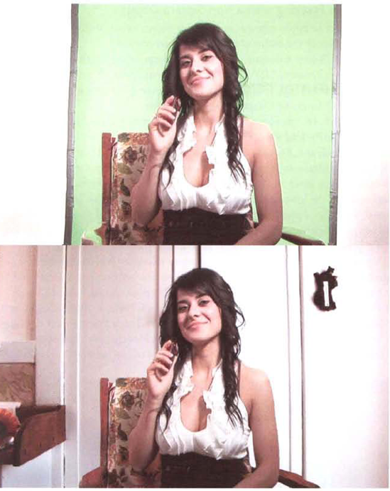
Masking is a necessary step for most compositing jobs. Even if rotoscoping is not required, a garbage matte is often needed to remove unwanted elements from footage. As such, you'll have a chance to clean up the greenscreen removal started in the Chapter 3 tutorial. In addition, you'll have the opportunity to corner pin motion track video footage.
In the Chapter 3 tutorial, you removed the greenscreen from a piece of video footage. However, additional masks must be drawn to remove the unwanted walls and to restore the missing arms of the chair.
Reopen the completed After Effects project file for "AE Tutorial 3: Removing Greenscreen." A finished version of Tutorial 3 is saved as
ae3.aepin the Chapter 3 Tutorials folder on the DVD. Scrub through the animation. At this stage, the walls remain on the left and right side. In addition, the chair arms are transparent due to the reflection of the greenscreen. Finally, the edges are not as clean as they could be.Open Comp 2 so that it's visible in the Timeline panel. Select the lower
phonecall.###.tgalayer (numbered 3 in the layer outline). Using the Pen tool, draw a mask around the model's hair (see Figure 7.31). Expand the Mask 1 section of the layer in the layer outline and toggle on the Stopwatch button beside the Mask Shape property. Move through the timeline and adjust the shape of the path so that the hair remains within the mask but the cell phone and the model's hand are never included. This step limits the effect of the luma matte and removes a dark line at the edge of the chair and the model's arm.Select the upper
phonecall.###.tgalayer (numbered 2 in the layer outline). Using the Pen tool, draw a U-shaped mask around the walls (see Figure 7.31). Expand the Mask 1 section and select the Inverted check box beside the Mask 1 property. The walls are removed.Import
room.tiffrom the Footage folder on the DVD. LMB+dragroom.tiffrom the Project panel to the layer outline of the Comp 2 tab in the Timeline panel so that's the lowest layer. Toggle off the Video layer switch beside the red Solid layer to hide it. The model appears over the background photo.The holes left in the arms of the chair are the last problem to solve. The holes exist because the wood reflected the greenscreen so strongly that the wood detail was obliterated. In this situation, it's necessary to add a small matte painting. Import the
touchup.tgafile from the Footage folder on the DVD. LMB+dragtouchup.tgafrom the Project panel to the layer outline of the Comp 2 tab in the Timeline panel so that it's the highest layer. Since touchup.tga is a full frame of the video, the chair arms must be isolated.With the touchup.tga layer selected, use the Pen tool to draw several paths around the two chair arms (see Figure 7.32). Since the model moves through the footage, you will need to animate the paths changing shape over time.
Using the Render Queue, render a test movie. If necessary, adjust the mask shapes and various filters to improve the composite. Once you're satisfied with the result, the tutorial is complete (see Figure 7.33). A finished revision is saved as ae3_final.aep in the Tutorials folder on the DVD.
In the Chapter 4 follow-up tutorial, you improved the greenscreen removal around the model's hair by creating a luma mask. However, additional masks must be drawn to remove the unwanted walls and to restore the missing arms of the chair.
Reopen the completed Nuke project file for "Nuke Tutorial 3 Revisited: Creating a Luma Matte." A matching version of Tutorial 3 is saved as
nuke3_step2.nkin the Chapter 4 Tutorials folder on the DVD. Scrub through the animation. At this stage, the walls remain on the left and right side. In addition, the chair is missing parts of its arms due to the reflection of the greenscreen. Finally, the matte edges are not as clean as they could be.With no nodes selected, RMB+click and choose Draw → Bezier. Rename the Bezier1 node HairMask through the node's Name cell. Connect the output of HairMask to the Mask input of the Merge1 node. Move the timeline to frame 1. With the HairMask node's properties panel open, Ctrl+Alt+click in the viewer to draw a path around the model's hair (see Figure 7.34). Animate the path over time by advancing to additional frames and moving the path vertices. The goal is to remove everything beyond the edge of the model's hair. Note that her hand is intentionally left out of the mask area.
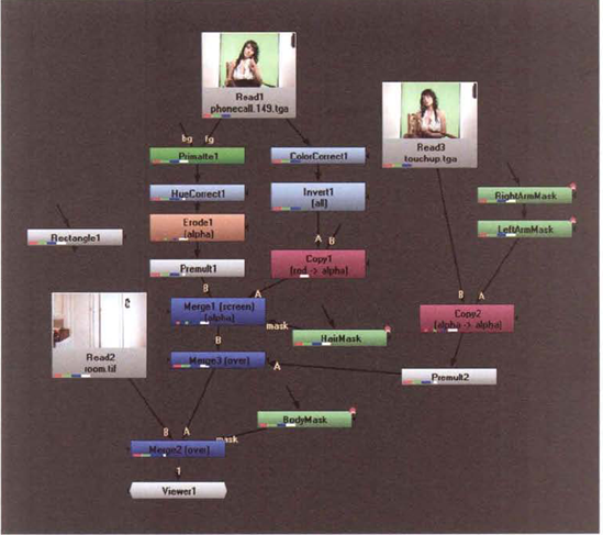
With no nodes selected, RMB+click and choose Draw → Bezier. Rename the new Bezier node BodyMask through the node's Name cell. Connect the output of BodyMask to the Mask input of the Merge2 node. Use Figure 7.35 as reference for the node network. The BodyMask node allows you to remove the unwanted walls with a second garbage matte. With the BodyMask node's properties panel open, Ctrl+Alt+click to draw a path around the walls in a U shape (see Figure 7.34). Select the Invert check box. The walls are removed.
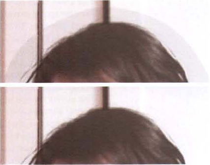
Disconnect the Rectangle1 node. With no nodes selected, RMB+click and choose Image → Read. Open the Read2 node's properties panel and browse for the
room.tiffile in the Footage folder on the DVD. Connect input B of the Merge2 node to the output of the Read2 node. A photo of a room is placed behind the model. Since the room is white, a dark halo close to the model's hair is revealed (see Figure 7.36). This is generated by the luma matte created by the ColorCorrect1, Invert1, and Copy1 nodes. The luma matte is a soft matte that maintains the detail of the hair but leaves a noisy alpha channel. To remove this noise, open the ColorCorrect1 node's properties panel and change the Gamma slider to 0.8 and the Gain slider to 2.2 (see Figure 7.36).The holes left in the arms of the chair are the last problem to solve. The holes exist because the wood reflected the greenscreen so strongly that the wood detail was obliterated. In this situation, it's necessary to add a small matte painting. With no nodes selected, RMB+click and choose Image → Read. Open the Read3 node's properties panel and browse for the
touchup.tgafile in the Footage folder on the DVD. Connect a viewer to the Read3 node. The image is taken from the first frame of the sequence. However, the arms of the chair have been restored through Photoshop painting (see Figure 7.37). Sincetouchup.tgais a full frame of the video, the chair arms must be isolated.With no nodes selected, RMB+click and choose Draw → Bezier. Rename the new Bezier node RightArmMask through the node's Name cell. With no nodes selected, RMB+click and choose Draw → Bezier. Rename the new Bezier node LeftArmMask through the node's Name cell. Connect the output of RightArmMask to the input of LeftArmMask. With no nodes selected, RMB+click and choose Channel → Copy. Connect the output of LeftArmMask to input A of the Copy2 node. Connect the output of the Read3 node to input B of the Copy2 node. With the Copy2 node selected, RMB+click and choose Merge → Premult. Connect a viewer to the Premult2 node. This series of connections allows you to draw a mask for the right arm, draw a mask for the left arm, merge them together, and use the resulting matte to separate the arms from the matte painting image. To draw the first mask, open the RightArmMask node's properties panel and Ctrl+Alt+click to draw a path around the right chair arm. Since the model moves through the shot and covers this arm, the path must be animated over time. To draw the second mask, open the LeftArmMask node's properties panel and Ctrl+Alt+click to draw a path around the left chair arm. The last few frames of this path will require animation as the model swings out her hand. Once both masks are drawn, the result is an isolated pair of chair arms (see Figure 7.37).
With no nodes selected, RMB+click and choose Merge → Merge. LMB+drag the Merge3 node and drop it on top of the connection line between Merge1 and Merge2. This inserts the Merge3 node after Merge1 and before Merge2. Connect input A of Merge3 to the output of Premult2. This places the isolated arms over the remainder of the composite, thus filling in the holes.
Test the composite by selecting the Merge2 node and choosing Render → Flipbook Selected. If necessary, make adjustments to the mask, color correction, or greenscreen removal nodes. Once you're satisfied with the result, the tutorial is complete (see Figure 7.38). A finished revision is saved as
nuke3_final.nkin the Tutorials folder on the DVD.
Corner pin tracking is easiest to apply when a rectangular object exists within a piece of footage. However, you can apply the technique to odd shaped objects.
Create a new project. Choose Composition → New Composition. In the Composition Settings dialog box, set Preset to HDV/HDTV 720, Duration to 30, and Frame Rate to 30. Import the
hydrant##.tgafootage from the Chapter 4 Footage folder on the DVD. Importsign.tiffrom the Chapter 7 Footage folder.LMB+drag the
hydrant.##.tgafootage from the Project panel to the layer outline of the Timeline panel. LMB+dragsign.tiffrom the Project panel to the layer outline so that it sits above thehydrant.##.tgalayer. The goal of this tutorial is to track the sign to the side of the fire hydrant so it looks like it was in the scene from the start.Select the
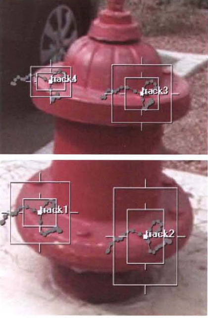
hydrant##.tgalayer and choose Animation → Track Motion. The Tracker Controls panel opens at the lower-right side of the program. Change the Track Type menu to Perspective Corner Pin. Four track points appear in the viewer of the Layer panel.Although corner pin tracking usually entails the positioning of four track points over the corners of a square or rectangular object, such as a TV screen, billboard, window, and so on, it's possible to apply corner pin tracking to whatever has four distinct features arranged in a rectangle manner. For instance, the fire hydrant has a series of bolts on the base and top lip that you can use for this purpose. As such, move Track Point 3 over the left base bolt (see Figure 7.39). Move Track Point 4 over the right base bolt. Move Track Point 2 over the top-right lip bolt. Move Track Point 1 over the top-left lip bolt. Scale each of the track point icons so they fit loosely over their respective bolts. If the icons fit too tightly, the tracker may lose sight of the bolts.
Press the Analyze Forward button in the Tracker Controls panel. The tracker moves through the footage one frame at a time. If it's successful, a motion path is laid for each track point (see Figure 7.39). If the tracker fails, adjust the track point positions and region sizes using the trouble-shooting suggestions in the section "Motion Tracking Problem Solving" earlier in this chapter.
Once you're satisfied that the tracking and motion paths exist for the entire duration of the timeline, click the Apply button in the Tracker Controls panel. The animation curves are automatically transferred to the
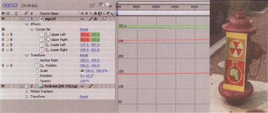
sign.tiflayer. (Since thesign.tiflayer sits above thehydrant.##.tgalayer, it's automatically assigned as the target layer.) Note that the view automatically changes to the viewer of the Composition panel when the Apply button is pressed. Henceforth, the sign appears properly scaled and skewed over the side of the hydrant (see Figure 7.40). Play back the timeline.At this stage, the sign is stretched over the top lip of the hydrant. To avoid this, you can offset the top tracking points. In the layer outline, expand the new Corner Pin section of the
sign.tiflayer. Toggle on the Include This Property In The Graph Editor Set button for the Upper Left and Upper Right properties. Toggle on the Graph Editor composition switch. Convert the Graph Editor to the value graph view by changing the Choose Graph Type And Options menu to Edit Value Graph. Click the Fit All Graphs To View button to frame all the curves. (The button features two lines surrounded by brackets.) The Upper Left Y and Upper Right Y curves are colored green. Draw a selection marquee around all the keyframes for the two Y curves. (Although the X curve keyframes become highlighted, they are not affected.) LMB+click one of the selected Y curve keyframes and drag the curves straight up. The top of the sign will move in the viewer of the Composition panel as you do this. Release the mouse button once the top of the sign is just below the top of the hydrant lip (see Figure 7.41).Toggle off the Graph Editor composition switch to return to the timeline view. Play back the footage. The sign remains sharper than the background footage. To add motion blur, toggle on the
sign.tiflayer's Motion Blur layer switch. To see the blur in the viewer, toggle on the Motion Blur composition switch. The blur will also appear when the composition is rendered through the Render Queue.

The tutorial is complete. A sample After Effects project is included as ae7.aep in the Tutorials folder on the DVD.
Corner pin tracking is easiest to apply when a rectangular object exists within a piece of footage. However, you can apply the technique or odd shaped objects.
Create a new script. Choose Edit → Project Settings. Change Frame Range to 1, 30 and Fps to 30. With the Full Size Format menu, choose New. In the New Format dialog box, change Full Size W to 1280 and Full Size H to 720. Enter a name, such as HDTV, into the Name field and click the OK button.
In the Node Graph, RMB+click and choose Image → Read. Open the Read1 node's properties panel and browse for
hyrdant.##.tgain the Chapter 4 Footage folder. With no nodes selected, choose Image → Read. Open the Read2 node's properties panel and browse forsign.tifin the Chapter 7 Footage folder. The goal of this tutorial will be to track the sign to the side of the fire hydrant so it looks like it was in the scene from the start.With the Read1 node selected, RMB+click and choose Transform → Tracker. Open the Tracker1 node's properties panel. While the Tracker tab is open, select the Enable check box beside Tracker 2, Tracker 3, and Tracker 4. Select the T, R, and S check boxes for all four trackers. Switch to the Settings tab and change the Warp Type menu to Translate/Rotate/Scale.
Change the timeline to frame 1. Switch back to the Transform tab. (If the Transform tab is not visible, the track anchor icons are hidden in the viewer.) Although corner pin tracking usually entails the positioning of four anchors over the corners of a square or rectangular object, such as a TV screen, billboard, window, and so on, it's possible to apply corner pin tracking to whatever has four distinct patterns arranged in a rectangular manner. For instance, the fire hydrant has a series of bolts on the base and top lip that you can use for this purpose. As such, place the Track1 anchor over the left base bolt (see Figure 7.42). Place the Track2 anchor over the right base bolt. Place the Track3 anchor over top-right lip bolt. Place the Track4 anchor over the top-left lip bolt. Scale each of the anchors so they fit loosely over their respective patterns. If the anchor regions are too tight, the tracker may lose track of the pattern.
Click the Track To The Last Frame button. The program steps through the footage one frame at a time. If the program stops short of frame 30, the tracker has lost one of the patterns. To avoid this, follow the problem-solving suggestions set forth in the section "Match-Move and Add Jitter Workflow" earlier in this chapter.
Once you're satisfied with the motion track calculation, choose the Read2 node, RMB+click, and choose Transform → CornerPin. With no nodes selected, RMB+click and choose Merge → Merge. Connect Read1 to input B of Merge1. Connect CornerPin2D1 to input A of Merge1. Connect a viewer to Merge1. The sign graphic appears at the left of the frame. To apply the motion tracking information to the sign, you must link the Tracker1 node to the CornerPin2D1 node.
Open the properties panels for the new CornerPin2D1 node and the Tracker1 node. The CornerPin2D1 node is designed to take tracking data from another node and cannot create tracking data on its own. Thus, you must create links to retrieve information from the Tracker1 node. To do so, Ctrl+LMB+drag the mouse from the Animation button beside Track1 in the Tracker tab of the Tracker1 node to the Animation button beside the To1 cells in the CornerPin2D tab of the CornerPin2D1 node. This creates a link between the two Animation buttons. (For more information on linking, see Chapter 12, "Advanced Techniques.") The link is indicated by the To1 cells turning a gray blue and a green arrow line appearing between the Tracker1 node and the CornerPin2D1 node (see Figure 7.43). In addition, a small green dot appears at the lower-right side of the CornerPin2D1 node with a small letter E, indicating that a link expression exists. Repeat the process of linking Track2 and To2, Track3 and To3, and Track4 and To4. As you create the links, the sign image is stretched and distorted until each of its corners touch corresponding track anchors. Note that the Transform menu of the Tracker1 node remains set to None.
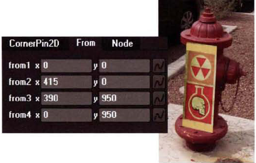
Play back the timeline using the viewer controls. Since the sign corners meet the anchors, the top of the sign is stretched over the lip of the hydrant. You can offset the effect of this stretching by switching to the From tab of the CornerPin2D1 node and entering new values into the From1, From2, From3, and/or From4 X and Y cells (see Figure 7.44). For example, to lower the top of the sign, change From3 Y and From4 Y to 950. You can also adjust the horizontal stretch of the sign by changing From2 X to 415 and From3 X to 390. This makes the sign more rectangular and less trapezoidal.
At this stage, the sign is much sharper than the background. You can activate motion blur for the CornerPin2D1 node by setting the Motion Blur slider, found in the CornerPin2D tab, to 1.0. Motion blur has a tendency to exaggerate minor imperfections in the tracking, however, especially when the motion is relatively subtle. For a less drastic result, change the Filter menu to Notch, which is an inherently soft interpolation method.
If imperfections remain in the tracking, you can continue to adjust anchor positions and use the track play buttons of the Tracker1 node to update the tracking information. Because the CornerPin2D1 node is linked, it will automatically update. You can also edit the tracking curves generated by the Tracker1 node. To do so, click the Track1 Animation button in the Tracker tab and choose Curve Editor. Keep in mind that the CornerPin2D1 node is using the Track1, Track2, Track3, and Track4 X and Y curves to determine the positions of the sign corners. It is not using Translate X, Translate Y, Rotate, or Scale W curves.
The tutorial is complete. A sample Nuke script is saved as nuke7.nk in the Tutorials folder on the DVD.
Born in Seoul, South Korea, Entae Kim attended Binghamton State University of New York. He switched majors from biology to graphic design and transferred to the Parsons School of Design. After graduation, he worked at several design firms as a web designer. He returned to the School of Visual Arts in New York to study 3D animation. In 2005, he began freelancing as a 3D generalist. Shortly thereafter, Entae joined the Freestyle Collective as head of the CG FX department. Since then, he's worked on numerous television commercials and network packages for clients such as the Cartoon Network, HBO, Nickelodeon, and Comedy Central.
Freestyle Collective is a collaborative design and production studio. Freestyle's services include creative advertising for commercial, broadcast, and corporate clients. Recent projects include identification spots for TCM, VH1, and MTV. The studio also sets aside resources for experimental animation, logo design, and print work.
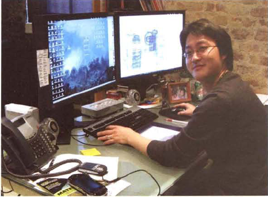
Entae Kim at his workstation (Photo courtesy of Freestyle Collective)
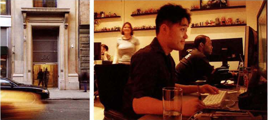
(Left) The Freestyle Collective office in the heart of Manhattan (Right) Freestyle Collective artists hard at work (Photos courtesy of Freestyle Collective)
(Freestyle Collective keeps five After Effects compositors on staff. The studio's sister company, New Shoes, runs additional Flame bays.)
LL: At what resolutions do you usually composite?
EK: We do a great deal of HD - 1080 (1920×1080). I'll say that 8 out of 10 [projects] are HD.
LL: So SD projects are fairly rare?
EK: It's always a good idea to work with HD since you can always down-convert [to SD].
LL: How have hi-def formats affected the compositing process?
EK: It's definitely been slow on the machine side-reading all these high-resolution files through a server. Also, adding effects and detail [means that] you have to double-check to make sure it works on the [HD] screen. When it was SD, you could get away with mistakes....
LL: Are there any special steps you take in preparation for color grading?
EK: Everyone here uses the same monitor—the same brand. They're calibrated once every week. You can actually correct them to look like NTSC color. Even with that, we bring the work into QC (quality control) monitors and check the vectorscope.
LL: What tools do you use to key blue- or greenscreen?
EK: After Effects has a great one—Keylight. But, almost always, you have to do some kind of roto. You always roto....
LL: Would you say the rotoscoping remains a common technique?
EK: All the postproduction houses have a team of rotoscopers.
LL: What tools do you use for tracking?
EK: Boujou. We sometimes use the After Effects tracking [tools].
LL: Do you use 2.5D or multiplane techniques?
EK: All the time. People want to get more dynamic camera motions. We actually have a matte painter, [so we] use 2.5D matte paintings with camera projections.
LL: Are there any limitations for using camera projections on cards or geometry?
EK: It only works for certain camera angles. It won't work [with] crazy moves through the scene, because the image is projected from the 3D camera onto the models you've set up.
LL: Do you prefer projecting on cards or geometry?
EK: It's better to use geometry, but it [doesn't have to] be super-detailed.
LL: Do you have 3D animators create the geometry?
EK: Yes, animators, modelers.... Normally, what we would do is set up the scene in 3D, render a couple of frames, give the [frames] to the matte painter—the matte painter will break down his layers in Photoshop, then give it to [the compositors], who project it from a 3D camera [in the composite]. It's 3D, then 2D, then it comes back into 3D.
LL: When you were in school, what style of compositing were you taught?
EK: Layers.... Now it's all 3D.
