
"Understand color and the way computers display images. Try to understand not just what buttons to push, but the underlying and relatively simple math that's happening under the hood."
Channel manipulation gives a compositor a great deal of control over every step of a composite. While alpha channels are the subject of considerable manipulation, other channels, such as color, luminance, and chrominance, are equally useful. After Effects and Nuke provide a wide array of channel manipulation effects and nodes, including those designed for channel copying and swapping, channel math operations, color space conversions, and color correction. To apply these tools successfully, it helps to understand the underlying math and modes of operations. To assist you in judging the result, histograms are an important device. To practice these concepts, this chapter includes After Effects and Nuke tutorials that integrate CG into degraded live-action footage. In addition, the Chapter 3 Nuke tutorial, which covers greenscreen removal, is revisited.
An image histogram is a graphical representation of tonal distribution. Histograms plot the number of pixels that possess a particular tonal value (that is, color) by drawing a vertical bar. The horizontal scale of a histogram runs from 0 to the total number of tonal steps. Therefore, the left side of a histogram represents shadow areas. The center represents mid-tones. The right represents highlights. For an 8-bit histogram, the horizontal values run left to right from 0 to 255. The vertical scale is generally normalized to run from 0 to 1.0. Histograms may represent a single channel or offer a combined view of all channels, such as RGB.

Figure 4.1. (Top) Overexposed digital image and matching histogram (Bottom) Properly exposed image with matching histogram. The bottom image is included as forest.tif in the Footage folder on the DVD.
With a histogram, you can quickly determine the quality of an image. For example, in Figure 4.1, an image is biased toward high tonal values, which indicates overexposure. In comparison, a more aesthetic exposure produces a more evenly graduated histogram.
With a low-contrast image, the pixels are concentrated in the center of the histogram. With a high-contrast image, the pixels are concentrated at the low and/or high ends. For example, in Figure 4.2, the same image of a forest is given a shorter exposure. Thus the histogram is biased toward the left. Because the sky in the upper left of the image remains overexposed, however, the last vertical line to the right of the histogram has significant height. The last line indicates pixels with a maximum allowable value. In the case of the example histogram, the value is 255, which implies that clipping is occurring.

Keep in mind that there is no "ideal" histogram. Histograms react to the subject that is captured. An image taken at dusk naturally produces a histogram biased toward the darker values. An image of an overcast day biases the histogram toward mid-tone values. An image of an intensely sunny day with deep shadows will form a bowl-shaped histogram with concentrations of pixels to the far left and far right. Nevertheless, there a few histogram features to avoid:
End Spikes If the first or last histogram line is significantly taller than neighboring lines, then clipping is occurring and potential detail is lost. For example, a spike at the far left of the histogram indicates that the darkest areas are 0 black with no variation.
Empty Areas If parts of the histogram are empty, then the image is restricted to a small tonal range. Although the image may appear to be fine, it won't be taking advantage of the full bit depth. While this is less likely to occur with a digital camera, compositing effects and nodes can induce such a histogram.
Combing A combed histogram is one that has regularly spaced gaps. Combing indicates that some tonal values have no pixels assigned to them. Combing occurs as a result of bit-depth conversions or the strong application of color correction effects and nodes. The only way to remove combing is to use a plug-in that's specifically designed for the task. (Combing and histogram repair plug-ins are discussed in Chapter 2, "Choosing a Color Space.") It's best to take steps to avoid excessive combing because it may lead to posterization (color banding). However, it's possible to reduce the impact of combing by applying noise and blur filters. This process is demonstrated in Chapter 8, "DI, Color Grading, Noise, and Grain."
Aside from quickly examining the tonal condition of an image, histograms are valuable for the process of color grading, whereby the color of footage is altered or adjusted in anticipation of delivery to a particular media, such as motion picture film or broadcast television. One important aspect of color grading is the establishment of a white point and a black point. A white point defines the value that is considered white. The term white is subjective in that human visual perception considers the brightest point in a brightly lit area to be white and all other colors are referenced to that point. A white point can be neutral, having equal red, green, or blue values, or it can be biased toward a particular channel. If a white point contains an unequal ratio of red, green, and blue, it may be perceived as white by the viewer nonetheless. To make the grading process more difficult, different media demand different black and white points for the successful transfer of color information. Note that white points and black points are often referred to as white references and black references when discussing logarithmic to linear conversions; for more information on such conversions, see Chapter 2. Color grading and the related process of digital intermediates are examined more closely in Chapter 8.
In many cases, the white point of a digital image is at the high end of the scale. With a generic, normalized scale, the value is 1.0. With an 8-bit scale, the value is 255. However, if the subject does not include any naturally bright objects, the white point can easily be a lower value, such as 200. Color correction effects and nodes allow you to force a new white point on an image and thus remap the overall tonal range. If the white point is 255, you can reestablish it as 225. The tonal range is thus changed from 0-255 to 0-225. A black point functions in the same manner, but establishes what is considered black. If a black point is 25 and a white point is 225, then the tonal range is 25-225.
A channel is a specific attribute of a digital image. Common channels include color and alpha. Whereas many compositing operations are applied to the red, green, and blue channels simultaneously, it often pays to apply an operation to a specific channel, such as the red channel or alpha channel.
After Effects offers 13 channel operation effects and 26 color correction effects as part of the Professional bundle. These are accessible via the Effect → Channel and Effect → Color Correction menus. The most useful effects are discussed in the following sections.
With Set Matte, Shift Channels, Set Channels, and Channel Combiner effects, you can move or copy one channel to another within a layer or between layers.
The Set Matte effect allows you to apply the value information of a channel or channels in one layer to the alpha channel of the same or different layer. This is particularly useful when an alpha matte is needed for a layer that currently does not possess one. For example, in Figure 4.3, a carved mask has overexposed highlights along its left forehead and cheek. In order to restore some color detail, two composites are set up. Comp 1 applies Levels and Fast Blur effects to isolate the highlights in the RGB. Comp 2 has the untouched footage as a lower layer and Comp 1 as an upper layer. Since Comp 1 does not have alpha information, a Set Matte effect is applied to it. The Take Matte From Layer menu defines the source used to create the alpha matte. In this example, it's set to Comp 1. The Use Matte For menu determines how the source will be used to generate the alpha matte. Options range from each of the color channels to alpha, luminance, lightness, hue, and saturation. In this example, the menu is set to Luminance, which produces a semitransparent matte. (For an additional example of the Set Matte effect, see "AE Tutorial 3: Removing Greenscreen" in Chapter 3, "Interpreting Mattes and Creating Alpha.")
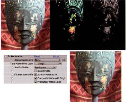
Figure 4.3. (Top Left) Unadjusted footage of mask (Top Center) Curves effect applied to isolate highlights (Top Right) Alpha matte generated by Set Matte effect (Bottom Left) Set Matte settings (Bottom Right) Final composite. A sample After Effects project is saved as set_matte.aep in the Tutorials folder on the DVD.
The Shift Channels effect replaces one channel with a different channel from the same layer. For example, in Figure 4.4, an image is given a surreal color palette by assigning the red, green, and blue channels to lightness, luminance, and green information respectively.
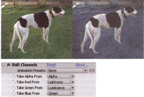
Figure 4.4. (Left) Unadjusted image (Right) The result of the Shift Channels effect (Bottom) Shift Channels settings. A sample After Effects project is saved as shift_channels.aep in the Tutorials folder on the DVD.
The Set Channels effect takes Shift Channels one step further by allowing you to define a different source for each of the RGBA channels. The sources can be the same layer or a different layer.
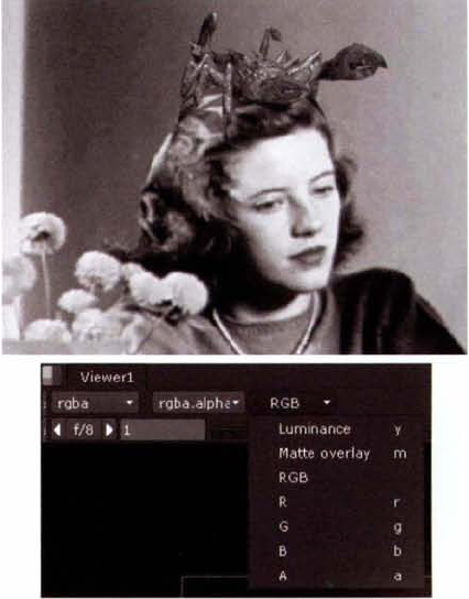
With the Channel Combiner effect, you can convert RGB color space to HLS or YUV color space. This is useful for any operation that needs to operate on a lightness, luminance, or chrominance channel. For example, to convert RGB to YUV, change the From menu to RGB To YUV. To examine the Y channel, change the viewer's Show Channel menu to Red (see Figure 4.5). The U channel is shown by switching to Green. The V channel is shown by switching to Blue. With YUV space, the Y channel encodes luminance, the U channel encodes the blue chroma component, and the V channel encodes the red chroma component. The green chroma component is indirectly carried by the Y channel. (For more information on YUV color space, see Chapter 3.)

Figure 4.5. (Top) Y luminance channel (Center) U blue chroma channel (Bottom) V red chroma channel. Note that the V channel contains the most noise.
In addition, you can premultiply an unpremultiplied layer by changing the From menu to Straight To Premultiplied. Much like the Shift Channels effect, you can also replace one channel with a different channel from the same layer. To do so, change the From menu to a channel you wish to borrow from and change the To menu to the channel you wish to overwrite. The Channel Combiner is demonstrated further in "AE Tutorial 4: Matching CG to Degraded Footage" later in this chapter.
With the Arithmetic and Calculations effects, you can apply standard math operations to the RGB values of a layer.
With the Arithmetic effect, A is the current pixel value of a channel and B is the value determined by the Red Value, Blue Value, or Green Value slider. The Operator menu sets the math operator to be used with A and B. For example, if Operator is set to Subtract and Red Value is set to 100, the following happens to a pixel with a red channel value of 150:
A - B = C
150 − 100 = 50
Thus, the new red channel pixel value is C, or 50. Note that the effect uses an 8-bit scale. This results in a reduction of red in the image and a relative increase of green and blue. As a second example, in Figure 4.6, the Operator menu is set to Difference, Red Value is set to 88, and Green Value is set to 162. Video footage of a lamp thus takes on psychedelic colors.
In this case, a pixel with a red value of 255 and a green value of 85 undergoes the following math:
absolute value of (255 − 88) = 167 (red)
absolute value of (85 − 162) = 77 (green)
The Difference operator takes the absolute value of A − B. Hence, the result is never negative. To ensure that none of the operators produce negative or superwhite values, the effect includes a Clip Result Values check box in the Effect Controls panel. If the check box is deselected, values above 255 are "wrapped around." For example, a value of 260 becomes 5.
The Operator menu offers 13 different operators. Add, Min, Max, Multiply, and Screen function like their blending mode counterparts (see Chapter 3 for descriptions). The mathematical equivalents of the remaining operators follow:
And:            If B < A then C = 0 else C = A
Or:             If B < A then C = A + B;
                If B > A then C = B
Xor:            If A = B then C = 0;
                If B < A then C = A + B;
                If B > A then C = B - A
Block Above:    If A > B then C = 0
Block Below:    If A < B then C = 0
Slice:          If A < B then C = 1.0 else = 0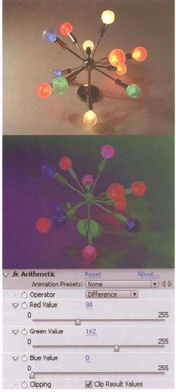
With the Calculations effect, you can apply blending modes to specific channels of different layers. For example, in Figure 4.7 a desert is blended with an abstract background (named ground.tif). The chosen blending mode, set by the Blending Mode menu, is Color Dodge. However, the blend only occurs between the red channel of the desert layer and the RGB of the abstract background layer.
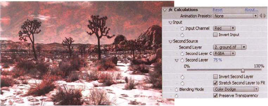
Figure 4.7. (Left) Desert image and abstract background blended with the Calculations effect (Right) Calculations settings. A sample After Effects project is saved as calculations.aep in the Footage folder on the DVD.
With blending mode math, the layer to which the Calculations effect is applied is layer A. You can choose layer B by selecting a layer name from the Second Layer menu. The channels used for A are set by the Input Channel menu. The channels used for B are set by the Second Layer Channel menu. The strength of layer B's influence is set by the Second Layer slider.
The Brightness & Contrast, Curves, Levels, Alpha Levels, Gamma/Pedestal/Gain, Hue/Saturation, Color Balance, and Broadcast Safe effects manipulate the value information of one or more channels. The effects, found in the Effect → Color Correction menu, can have a significant impact on value distribution and thus the shape of an image histogram. In this section, the histogram display of the Levels effect is used to demonstrate these changes.
The Brightness & Contrast effect shifts, stretches, or compresses tonal ranges. The Brightness slider value is added or subtracted to every pixel of the layer. For example, if Brightness is set to 10, 10 is added. If Brightness is set to −20, 20 is subtracted. Positive Brightness values have the effect of brightening the image while sliding the entire tonal range to the right of the histogram (see Figure 4.8). Negative Brightness values have the effect of darkening the image while sliding the entire tonal range to the left of the histogram. The results are clipped, so negative and superwhite values are not permitted.
Positive Contrast values stretch the tonal range. This has the effect of lowering values below the 0.5 median level and raising values above the 0.5 median level. Resulting values below 0 and above 1.0 are discarded. In addition, the higher the Contrast value, the greater the degree of combing that occurs (see Figure 4.8). As discussed in Chapter 2, combing can create unwanted posterization (color banding). Note that 8-bit, 16-bit, and 32-bit images all suffer from combing if the tonal range is stretched by the Contrast slider. However, posterization is more noticeable with an 8-bit image since there are fewer tonal steps to begin with. When the stretching occurs, a limited number of tonal steps are spread throughout the tonal range, which creates empty gaps in the histogram.
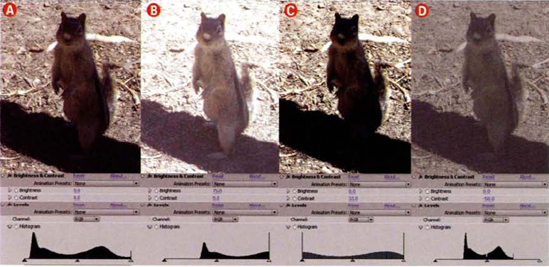
Figure 4.8. (A) Unadjusted image with corresponding Levels histogram. (B) A Brightness value of 75 pushes the tonal values to the right of the histogram. (C) A Contrast value of 33 stretches the tonal range, which leads to the loss of low and high values and a combing of mid-range values. (D) A Contrast value of −50 compresses the tonal range, leaving no low or high values. The image is included as squirrel.tif in the Footage folder on the DVD.
Negative Contrast values compress the tonal range. This has the effect of raising values below the 0.5 median level and lowering values above the 0.5 median level. You can equate the value of the Contrast slider with a percentage that the tonal range is stretched or compressed. For example, if the Contrast slider is set to −50, the tonal range is compressed down to 50%, or half its original size (see Figure 4.8). If the tonal range originally ran from 0 to 255, the new tonal range runs approximately from 64 to 192.
The Curves effect allows you to remap input values by adjusting a tonal response curve that has 256 possible points. By default, the curve runs from left to right and from 0 to a normalized 1.0. The horizontal scale represents the input tonal values and the vertical scale represents the output tonal values. The functionality is similar to the remapping undertaken by a LUT curve (see Chapter 2). If the curve is not adjusted, an input value of 0 remains 0, an input value of 0.5 remains 0.5, and so on. If you move the start or end points or add new points and reposition them, however, new values are output. (The curve start point sits at the lower left, and the curve end point sits at the upper right.)
For example, you can compress the tonal range toward the high end of the scale by pulling the start point straight up (see Figure 4.9). You can stretch the low end of the tonal range while clipping the high end by moving the end point to the left. You can approximate a gamma function by adding a point to the curve center and pulling it down. You can approximate an inverse gamma function (1 / gamma) by adding a point to the curve center and pulling it up. You can add contrast to the layer by inserting two points and moving the lower point toward 1.0 and the upper point toward 0.

Figure 4.9. (A) Image brightened by raising start point (B) Contrast reduced by pulling end point left (C) Inverse gamma curve approximated by inserting new point (D) Contrast increased by creating "S" curve with two new points
To insert a new point on the curve, LMB+click on the curve. To move a point, LMB+drag the point. To reset the curve to its default state, click the Line button. To smooth the curve and freeze current points, click the Smooth button. The Smooth button, which sits above the Line button, features an icon with a jagged line. To freehand draw the curve shape, select the Pencil button and LMB+drag in the graph area. You can save a curve and reload it into a different instance of the Curves effect by using the File Save and Open buttons. The Curves effect can operate on RGB simultaneously or on an individual channel, such as red or alpha; this is determined by the Channel menu. Note that extreme curve manipulation may lead to excessive posterization or solarization. (Solarization occurs by blending positive and negative versions of an image together.)
As demonstrated, the Levels effect features a histogram. You can adjust the histogram with Input Black, Output Black, Input White, Output White, and Gamma properties (see Figure 4.10). The adjustment is applied to either RGB or individual color and alpha channels, as determined by the Channel menu. Any input values less than the Input Black value are clamped to the Output Black value. If the Input Black value is 0.2, the Output Black value is 0.3, and if a pixel has an input value of 0.1, the pixel receives an output value of 0.3. Ultimately, the Output Black slider establishes the black point of the image (see the section "Tonal Ranges, White Points, and Black Points" earlier in this chapter). Any input values greater than the value of Input White slider are clamped to the Output White value. If the project is set to 8-bit, the maximum clamp value is 255. If the project is set to 16-bit (which is actually 15-bit with one extra step), the maximum clamp value is 32,768. The Output White slider establishes the white point of the image. (Note that the histogram only indicates 256 steps regardless of the project bit depth.) The Gamma slider sets the exponent of the power curve normally used to make the image friendlier for monitor viewing (see Chapter 2 for more information on gamma). If Gamma is set to 1.0, it has no effect on the image. If Gamma is lowered, mid- and high-tones are pulled toward the low end of the tonal range. If Gamma is raised above 1.0, the low and mid-tones are pulled toward the high end of the tonal range. A low Gamma value produces a high-contrast, dark image. A high Gamma value produces a washed-out, bright image.

Figure 4.10. (Top Left) Unadjusted image (Top Right) Corresponding Levels settings (Bottom Left) Image adjusted to bring out detail in shadows (Bottom Right) Corresponding Levels settings. The image is included as truck.tif in the Footage folder on the DVD.
In addition, you can interactively drag the handles below the histogram. The top-left handle controls the Input Black value. The top-right handle controls the Input White value. The top-center handle controls the Gamma value. The two handles below the black and white bar set the Output Black and Output White values. Moving the Input Black and Input White handles toward each other discards low and high values, stretches the mid-tones to fill the tonal range, and leads to combing. Moving the Output Black and Output White handles toward each other compresses the tonal range and leaves the ends of the histogram empty. Note that changing the various sliders or handles does not change the histogram shape, which always represents the tonal range of the input layer before the application of the Levels effect. If you wish to see the impact of the Levels effect on the image histogram, you can add a second iteration of the Levels effect and leave its settings with default values.
The Levels (Individual Controls) effect is available if you want to apply separate Input Black, Output Black, Input White, Output White, and Gamma settings for each channel.
The Alpha Levels effect (found in the Effect → Channel menu), allows you to adjust an alpha channel with Input Black Level, Output Black Level, Input White Level, Output White Level, and Gamma sliders. Its functionality is similar to the Levels effect, although it lacks a histogram and has no impact on the RGB channels.
The Gamma/Pedestal/Gain effect offers yet another means to adjust an image's tonal response curve. It splits its controls for the red, green, and blue channels but does not affect alpha. The Red/Green/Blue Pedestal sliders set the minimum threshold for output pixel values. Raising these slider values compresses the tonal range toward the high end. Lowering these slider values stretches the tonal range toward the low end, thus clipping the lowest values. The Red/Green/Blue Gain sliders set the maximum output pixel values. Lowering these slider values compresses the tonal range toward the low end. Raising these slider values stretches the tonal range toward the high end, thus clipping the highest values. The Red/Green/Blue Gamma sliders operate in the same manner as the Gamma slider carried by the Levels effect. The Black Stretch slider, on the other hand, pulls low pixel values toward median values for all channels. High Black Stretch values brighten dark areas. Since you can adjust each of the three color channels separately with the Gamma/Pedestal/Gain effect, you can alter the overall color balance. For example, in Figure 4.11, the colors are shifted to dusklike lighting.

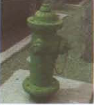
The Hue/Saturation effect operates on the HSL color wheel. It allows you to offset the image colors by interactively adjusting the Master Hue control. For example, if Master Hue is set to 120°, the primary red of a fire hydrant becomes primary green (see Figure 4.12). Setting it to 240° turns the hydrant blue. In terms of the resulting hues, 360° is the same as 0°. However, in order to support smooth keyframe animation, you can make multiple revolutions of the control. The revolutions are tracked as 1×, 2×, 3×, and so on.

Figure 4.12. (Left) Unadjusted image of hydrant (Center) Master Hue set to 120° (Right) Corresponding Hue/Saturation settings. The sample After Effects project is included as hue_saturation.aep in the Tutorials folder on the DVD.
With the Hue/Saturation effect, you can control the image saturation. (As mentioned in Chapter 3, saturation is the colorfulness of a color in reference to its lightness.) A high Master Saturation value, such as 75, creates a greater contrast between the RGB channels of a pixel. As a result, the dominant channels, whether they are red, green, or blue, are pushed closer to a value of 1.0 (normalized) or 255 (8-bit). The less-dominant channels are pushed closer to 0. For example, a pixel near the top of the hydrant in the unadjusted hydrant footage (seen at the left of Figure 4.12) has an RGB value of 158, 66, 85. This equates to a ratio of roughly 2.4:1:1.3 where the red channel is 2.4 times as intense as the green channel and the blue channel is 1.3 times as intense as the green channel. If the Saturation slider is set to 50, the pixel's RGB values change to 203, 20, 58 (see the top of Figure 4.13). Thus, the red channel becomes roughly 10 times as intense as the green channel and the blue channel becomes 2.9 times as intense as the green channel.

Figure 4.13. (Top) Master Saturation slider set to 50. (Center) Master Saturation slider set to 100. Note the appearance of noise and compression artifacts. (Bottom) A colorized version using a blue Colorize hue.
Master Saturation values less than 0 reduce the contrast between red, green, and blue channels. A Master Saturation value of −100 makes the balance between red, green, and blue channels equal, which in turn creates a grayscale image. A pixel at the top of the hydrant would therefore have a value of 112, 112, 112.
The Hue/Saturation effect offers a Colorize check box. If this is selected, the Master sliders are ignored. Instead, the image is tinted with a hue set by the Colorize Hue control (see the bottom of Figure 4.13). The tinting process increases or decreases channel values in preference of the set hue. For every 25% increase in the Colorize Saturation value, the channels increase or decrease in value by 25%. If Colorize Hue is primary red (0°), green (120°), or blue (240°), only a single channel is increased while the other two are decreased. However, if the hue is a secondary color, two channels are increased while the remaining channel is decreased. For example, a yellow hue (60°) increases the red and green channels while reducing the blue channel. If the hue is a tertiary color, one channel is increased, one channel is left at its input value, and one channel is decreased. For example, an orange hue (30°) increases the red, leaves the green static, and decreases the blue. (For more information on primary, secondary, and tertiary colors, see Chapter 2.)
The Color Balance effect shifts the balance between red, green, and blue channels. Balance sliders are provided for each channel and for three tonal zones (Shadow, Midtone, and Highlight). Negative Shadow slider values stretch the channel's tonal range toward the low end, clipping the lowest pixel values. Positive Shadow slider values shift the channel's tonal range toward the high end. Negative Midtone slider values shift the mid-tones toward the low-end without clipping. Positive Midtone slider values shift the mid-tones toward the high end without clipping. Negative Highlight slider values stretch the channel's tonal range toward the low end without clipping. Positive Highlight slider values shift the channel's tonal range toward the high end, clipping the highest pixel values.
The Color Balance (HLS) effect operates in a similar fashion to the Hue/Saturation effect. The Hue control offsets the layer colors. The Lightness property sets the brightness and the Saturation property sets its namesake.
The Exposure effect simulates an f-stop change. Although it is designed to adjust 32-bit high-dynamic range images (HDRIs), you can apply the effect to 8- or 16-bit layers. The Exposure slider sets the f-stop value, the Offset slider offsets the Exposure value, and the Gamma slider applies a gamma curve. For additional information, see Chapter 12, "Advanced Techniques."
The Broadcast Colors effect reduces values to a level considered safe for broadcast television. The amplitude of NTSC video is expressed in IRE units, as is the effect's Maximum Signal Amplitude slider. Values between 7.5 and 100 IRE units are considered safe for analog NTSC broadcast as they do not cause color artifacts. The IRE range is equivalent to an 8-bit range of 16 to 235. (See Chapter 2 for information on IRE units and After Effects support of 16-235 color profiles.) Values between 0 and 100 IRE units are considered safe for digital ATSC and DVB HDTV broadcast. You can choose a maximum IRE level by changing the Maximum Signal Amplitude slider. You can choose to reduce the image luminance, reduce the saturation, or key out unsafe areas by changing the How To Make Color Safe menu.
Nuke offers over two dozen channel operation, color correction, and math nodes. These are accessible via the Channel and Color menus. Before the most useful nodes are examined, however, a closer look at Nuke's channel and node controls is needed.
The majority of Nuke nodes carry Red, Green, and Blue channel check boxes. These are displayed beside the Channels menu (see Figure 4.14). When a channel check box is deselected, the channel is no longer affected. This is indicated by the Nuke node box itself. If the channel line symbol is short, it's not affected by the node. In other words, the channel is passed through the node without any processing. If the channel line symbol is long, it is affected by the node. An Alpha check box is also included, but only if the Channels menu is set to Rgba or Other Layers → Alpha.
At the same time, the majority of Nuke nodes carry a Mix slider (see Figure 4.15). Mix fulfills its namesake by allowing you to blend the output of the node with the unaffected input. This provides a quick means by which you can reduce the influence of a node without changing its specific sliders or menus.

Figure 4.14. :(Top) Channel check boxes (Bottom) Node box showing channel lines. Long lines for green and blue channels indicate that the channels are affected. Short lines for red and alpha channels indicate that the channels are unaffected. (Although not pictured here, the node box will include channel lines for any existing depth or UV channel.)
The Copy, ChannelMerge, ShuffleCopy, and Shuffle nodes provide the ability to transfer channels for a single input or between multiple inputs.
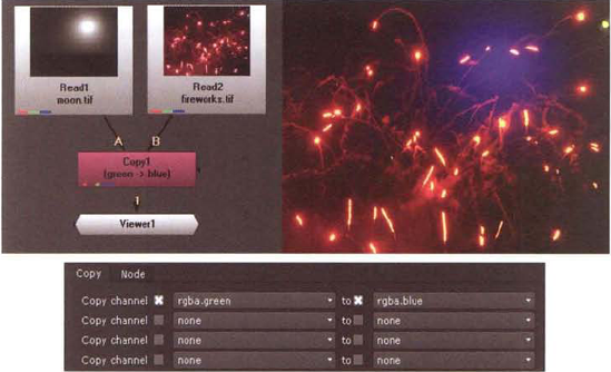
The Copy node allows you to copy one to four channels from one node to another node. The Copy node's input A is designed for connection to the node providing the channel information. The Copy node's input B is designed for connection to the node receiving the channel information. For example, in Figure 4.16, the green channel from an image of the moon is transferred and applied to the blue channel of a fireworks image.
For an additional example of the Copy node in a network, see "Nuke Tutorial 3 Revisited: Creating a Luma Matte" later in this chapter.
The ChannelMerge node is able to merge two channels. It provides a number of standard merging operations, such as plus, minus, multiply, min, and max. As an example, in Figure 4.17, two variations of a CG render are merged together. The first render is in grayscale and is connected to input A of the ChannelMerge node. The second render is in color and is connected to input B of the ChannelMerge node. The ChannelMerge node takes the red channel from A and multiplies it by the green channel of B.

Figure 4.17. (A) Grayscale render (B) Color render (C) Color render's green channel before the application of ChannelMerge (D) Color render's green channel after the application of ChannelMerge (E) Node network (F) ChannelMerge settings (G) Output of ChannelMerge node. A sample Nuke script is included as channelmerge.nk in the Tutorials folder on the DVD.
With the ShuffleCopy node, you can rearrange or swap channels between two input nodes and have the result output. Input 1 is fed into the In menu and input 2 is fed into the In2 menu (see the top of Figure 4.18). By default, the node uses the RGBA channels of the inputs; however, you can switch the In and In2 menu to another channel, such as alpha.
You can break the ShuffleCopy properties panel into four sections: InA, In2A, InB, and In2B (see the top of Figure of 4.18). If a channel check box is selected in an In section, then that channel is used for the output, but only for the channel for which it's selected. For example, if the lowest red check box in the InA section is selected, then the red channel is fed into the alpha channel of the output (see the bottom of Figure 4.18).

Figure 4.18. (Top) The four sections of the ShuffleCopy properties panel (Bottom) A red channel check box, in the InA section, is sent to the output's alpha channel.
By selecting various check boxes in the InA, In2A, InB, and In2B sections, you can quickly rearrange channels. For example, in Figure 4.19, two Read nodes are connected to a ShuffleCopy node. The ShuffleCopy node's check boxes are selected so that the output's red channel is taken from Read2's red channel, the output's green channel is taken from Read1's red channel, and the output's blue channel is taken from Read1's blue channel. Thus the fireworks image loaded into the Read2 node provides only red channel information. In the meantime, the moon image loaded into Read1 has its channels scrambled. This results in red, low-intensity fireworks over a cyan moon.
The ShuffleCopy node's output is ultimately determined by the two output menus, named Out and Out2 (see the top of Figure 4.18). By default, the Out2 menu is set to None. In this case, the InB and In2B sections are nonfunctional. If the Out2 menu is set to specific channels, then the InB and In2B sections become active and add additional processing to the original inputs. If the Out2 channel matches the Out menu, however, Out2 overrides Out. If the Out2 channel is different, then both outputs are able to provide up to eight processed channels. For example, if Out is set to Rgb and Out2 is set to Alpha, the InA and In2A sections create the color while the InB and in2B sections create the alpha information. For example, in Figure 4.20, the output red channel is derived from the green channel of input 2. The output green channel is derived from the green channel of input 1. The output blue channel is derived from the blue channel of input 2. The output alpha channel is derived from the green channel of input 1. Note that the ShuffleCopy node has only one output when connected in a node network. The single output can carry up to eight channels so long as the channels are unique.
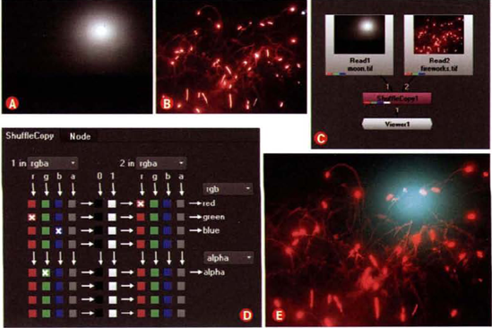
Figure 4.19. (A) Long-exposure shot of moon (B) Footage of fireworks (C) ShuffleCopy node connected to Read nodes (D) ShuffleCopy properties panel (E) Resulting composite. A sample Nuke script is saved as shufflecopy.nk in the Tutorials folder on the DVD.

Figure 4.20. (Left) ShuffleCopy settings with Out set to Rgb and Out2 set to Alpha (Top Right) RGB result (Bottom Right) Alpha result. A sample Nuke script is included as shufflecopy_2.nk in the Tutorials folder on the DVD.
Aside from Rgb, Rgba, and Alpha, you can set the Out and Out2 menus to Depth, Motion, Forward, Backward, or Mask layers (for example, Other Layers → Depth). Depth is designed for Z-buffer renders and provides a Z channel. Motion is designed for motion vector information and comes with two sets of UV channels: one for forward and one for backward motion blur. The Forward layer carries the forward UV portion of motion vector information. The Backward layer carries the backward UV portion of motion vector information. The Mask layer is designed to read a matte channel that is separate from standard alpha. Depth, Motion, Forward, Backward, and Mask layers and channels are discussed in more detail in Chapter 9, "Integrating Render Passes."
To create a total of eight output channels with the ShuffleCopy node, set one output menu to Rgba and one output menu to Motion. Otherwise, you will need to create a custom layer that carries four channels. To do so, set the Out or Out2 menu to New. In the New Layer dialog box, change the top four Channels menus to channels of your choice.
In addition, ShuffleCopy offers two "constant" channels. These are labeled 0 and 1 in the center of the properties panel. If a 0 check box is selected, it supplies the corresponding output channel a value of 0. If a 1 check box is selected, it supplies the corresponding output channel a maximum value (such as 1.0 on a normalized scale).
The Shuffle node looks identical to the ShuffleCopy node. However, it's designed for only one input. Thus, it's appropriate for rearranging and swapping channels within a single image.
The Colorspace, HueShift, and HSVTool nodes are able to convert between color spaces.
The Colorspace node converts an input from one color space to another. Its In set of menus establish the interpretation of the incoming data and its Out menus determine the outgoing conversion. The leftmost column of the menus sets the color space (see Figure 4.21).
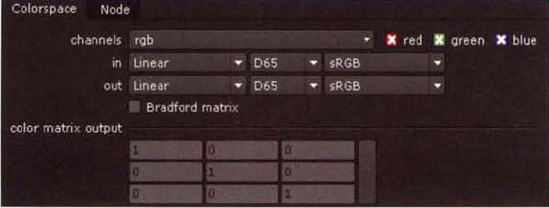
If the In menu is set to default Linear, the input data is accepted as is with no filtering. If the In menu is set to a specific space, then the program assumes the data matches that space. For instance, if the menu is set to HSV, the program interprets the red channel as hue, the blue channel as saturation, and the green channel as value.
By default, any image or image sequence imported into Nuke has a LUT applied to it. The LUT is determined by the LUT tab of the Project Settings properties panel. For example, 8- and 16-bit images have a sRGB LUT applied to them. You can override this behavior when preparing to use the Colorspace node by changing the Read node's Colorspace menu to Linear. Also note that the viewer uses a display LUT by default, which may interfere with the proper viewing of the Colorspace output. To avoid this, you can change the Display_LUT menu to Linear as well.
If the Out menu is set to default Linear, then the node is disabled. However, if the Out menu is set to one of the other 14 color spaces, the channels are reorganized, a log-to-linear conversion occurs, a LUT is applied, or a gamma curve is applied. For example, if L*a*b* is chosen, the RGB channels are converted to an L* luminance channel and a* and b* chroma channels. If Cineon is chosen, an internal linear-to-log conversion occurs. If Rec709 (∼1.95) is chosen, the Rec709 LUT is applied utilizing a gamma of 1.95.
Other color spaces, which have not yet been discussed, include YPbPr, CIE-LCH, CIE-XYZ, and CIE-Yxy. YPbPr is an analog variation of Y'CbCr. CIE-LCH is a lightness-saturation-hue-based color space. CIE-XYZ was defined in 1931 and continues to serve as the basis for modern RGB color spaces. X, Y, and Z correspond to tristimulus values that approximate red, green, and blue primary colors. (Tristimulus values are the amounts of three primary colors in a 3-component additive color system that are needed to represent a particular color.) CIE-Yxy is formulated from CIE-XYZ color space and is commonly represented by a horseshoe or "shoe sole" chromaticity chart (see the next section for an example). With CIE-Yxy, Y represents luminance, while x and y are coordinates that identify the hue/chroma component. Hue is the main property of a color. Specific hues correlate to specific wavelengths of light. Colors with primary hues are given names such as red, green, and blue. Chroma is the colorfulness of a color in reference to perceived white (which varies with the environment). Colorfulness is the degree to which a color is different from gray at a given luminance. Note that CIE-Yxy is often written as CIE-xyY.
The second column of menus controls the illuminant used. Illuminants are standardized profiles that allow images produced under different lighting conditions to be accurately compared. An illuminant profile contains numeric information that represents the spectral quality of a specific light source. Common profiles have been established by the CIE (International Commission on Illumination). When an RGB-based color space is defined, the coordinates of color primaries and a white point (white reference) are established. For example, sRGB color space uses the D65 illuminant to determine the location of the white point. The D65 illuminant replicates midday sun and has a correlated color temperature (CCT) of just over 6500 K. In general, the illuminant menu should match the corresponding color space. For instance, Wide Gamut RGB uses the D50 illuminant (5003 K) and NTSC RGB uses the C illuminant (6774 K).
The third column of menus establishes the color primaries used in the color space conversion. Color primaries are numerically-expressed locations within Yxy color space that identify each primary color. For example, sRGB color space assigns its red primary an Yxy location of 0.64 (x), 0.33 (y). In contrast, the SMPTE-C RGB color space assigns its red primary an Yxy location of 0.63 (x), 0.34 (y). (SMPTE-C refers to a color standard set by the Society of Motion Picture and Television Engineers.) Although the visual difference between various color primary settings may be slight, selecting a new primary will alter the numeric values of the output. In general, the color primaries menu should match the corresponding color space. For example, if you are converting to HDTV color space, set the Out menus to Rec709(∼1.95), D65, sRGB. For a demonstration of the Colorspace node, see "Nuke Tutorial 4: Matching CGI to Degraded Footage" later in this chapter.
The HueShift node converts the input color space to CIE-XYZ. To visualize the CIE-XYZ color space, CIE-Yxy chromaticity charts are used (see Figure 4.22). With the chart, x runs horizontally, y runs vertically, and Y runs on an axis perpendicular to the xy plane and points toward the viewer. While x and y coordinates define the hue/chroma component of a color, Y determines the luminance. The white point of the space is located within the central white spot. Note that the chart is actually a flat, 2D representation of a curved color space.

With the HueShift node, the Hue Rotation slider rotates the color space around the Y axis. The pivot of the rotation is located at the white point. For example, a Hue Rotation value of 180 turns red into cyan. Positive Hue Rotation values rotate the Yxy chart in a clockwise fashion. The Saturation parameter controls standard saturation, while the Saturation Along Axis parameter controls the saturation along either a red, green, or blue axis as determined by the Color Axis cells. Each color axis runs from a corner of the chromaticity diagram toward the white point. You can select an axis between primary colors by clicking the Color Sliders button beside the Color Axis cells and choosing a non-primary color. The Input Graypoint and Output Graypoint parameters offset color values in order to maintain a proper gray mid-tone; the parameters may be left at a default 0.25.
The HSVTool node converts the input color space to HSV color space. As such, it provides a section of parameters for the hue, saturation, and value components. For example, the Hue section includes a Rotation slider that offsets the hue value. The Saturation section includes an Adjustment slider to set the intensity of the saturation. The Brightness section includes an Adjustment slider to determine the brightness. Each section includes Range controls, which you can adjust to limit the effect of a node to a narrow input value range. The HSV Tool node converts the adjusted values back to the input color space in preparation for output.
Color correction nodes include Saturation, Histogram, Grade, ColorCorrect, and HueCorrect.
The Saturation node controls its namesake. A high Saturation property value, such as 2, creates a greater contrast between the RGB channels of a pixel. As a result, the dominant channels, whether they are red, green, or blue, are pushed closer to a value of normalized 1.0. The less-dominant channels are pushed closer to 0. For example, in Figure 4.23, an input gains greater contrast when Saturation is set to 2. As such, the green values are reduced to 0 along the truck body because the body is heavily biased towards red.

Figure 4.23. (Left) Green channel before application of Saturation node (Right) Green channel after application. The Saturation slider is set to 2 and the Luminance Math menu is set to Maximum. The image is included as truck.tif in the Footage folder on the DVD.
You can choose the style of saturation or desaturation by changing the Luminance Math menu. The CCIR 601 menu option uses a digital video and computer graphics standard that's biased for human perception, which has the formula Y = 0.299 red + 0.587 green + 0.114 blue. The Rec 709 menu option uses a variation of the CCIR standard and is written as the formula Y' = 0.2126 red' + 0.7152 green' + 0.0722 blue'. (For more information, see the Tips & Tricks sidebar about brightness, lightness, luminance, and luma earlier in this chapter.) Of the four menu options, the Maximum menu option applies the maximum amount of contrast between the channels.
The Histogram node provides a means to adjust black and white points of an input and its overall tonal range. (See the section "Histograms and Tonal Ranges" earlier in this chapter for more information on points.) There are two sets of sliders: Input Range and Output Range. The leftmost slider handle for Input Range serves as a black value input. Any input values less than the handle value are clamped to the handle value. The rightmost slider handle for Input Range serves as a white value input. Any input values greater than the handle value are clamped to the handle value. Thus, any adjustment of these two sliders will cause a section of the tonal range to be lost. However, the remaining tonal range is stretched to fill the entire histogram. The center slider for Input Range applies a gamma-correction curve; if set to 1.0, the correction is disabled. Movement of the leftmost or rightmost slider will cause the center slider to move automatically. Note that the histogram graphic will superimpose the newly adjusted tonal distribution over the original tonal distribution. The position of the black value input is indicated by a white line that extends the height of the histogram on the histogram's left. The position of the white value input is indicated by a white line that extends the height of the histogram on the histogram's right. (If the histogram graphic does not update, try clicking the graphic or closing and opening the properties panel.)
The leftmost slider for Output Range determines the image's black point. The rightmost slider for Output Range determines the image's white point. The position of the black point is indicated by a black line that extends the height of the histogram on the histogram's left. The position of the white point is indicated by a black line that extends the height of the histogram on the histogram's right. If either the white point or black point is adjusted, the tonal range is compressed and a section of the histogram will remain empty. For example, in Figure 4.24, an image of a squirrel is adjusted with various Histogram node settings.

Figure 4.24. (Top) Unadjusted image with histogram (Center) Washed-out version created by raising the black point and lowering the white point (Bottom) Properly exposed version with an 0.7 gamma, lowered white input value, and lowered white point. A sample Nuke script is included as histogram.nk in the Tutorials folder on the DVD.
The Grade node provides a more powerful means to adjust the black point, white point, gain, and gamma of an image. The black point, white point, gain, and gamma are predictably controlled by the sliders with the same name (see Figure 4.25). In addition, Lift, Offset, and Multiply sliders are provided for greater fine-tuning.
Since the slider scales are unintuitive, here are some approaches to keep in mind when adjusting them:

Although there is no slider for pedestal, negative Blackpoint slider values are equivalent to positive pedestal values, whereby the values are compressed toward the high end of the tonal range. Positive Blackpoint slider values are equivalent to negative pedestal values. In such a situation, low-end values are clipped and the remaining values are stretched to fit the tonal range.
Positive Gain slider values create traditional gain, whereby high-end values are clipped and the remaining values are stretched to fit the tonal range.
If Whitepoint is set above 1.0, the tonal range is compressed toward the low-end of the scale and the upper-end of the range is left empty.
A positive Lift value produces an almost identical result as a negative Blackpoint value. A negative Lift value produces an almost identical result as a positive Blackpoint value.
A positive Offset value produces an almost identical result as a negative Blackpoint value. However, negative Offset values produce results similar to a Whitepoint value above 1.0, but the image is darkened.
High Multiply values increase the brightness of an image and reduce the overall contrast.
To enter specific numeric color values for a slider, click the 4 button beside the slider.
To choose a color for a slider interactively, click the Color Sliders button beside the slider name (the button features a small color wheel).
The Grade node will be examined further in Chapter 8, "DI, Color Grading, Noise, and Grain."
The ColorCorrect node controls the balance between red, green, and blue channels within an image. Saturation, Contrast, Gamma, Gain, and Offset sliders are provided. These sliders function in the same manner as the ones provided by other color correction nodes and effects, but are targeted toward finite sections of the tonal range (Shadows, Midtones, and Highlights). In addition, a "Master" set of sliders control the entire tonal range. The ColorCorrect node is demonstrated in "Nuke Tutorial 4: Matching CG to Degraded Footage" later in this chapter.
The HueCorrect node controls the balance between red, green, and blue channels and offers an interactive curve editor with color control and suppression curves. Control curves are supplied for saturation, luminance, red, green, and blue thresholds. Suppression curves are supplied for red, green, and blue channels. The HueCorrect node is demonstrated in the "Nuke Tutorial 2 Revisited: Refining Color and Edge Quality" and "Nuke Tutorial 3: Removing Greenscreen" in Chapter 3.
Nuke provides basic math nodes, which are found under the Color → Math menu. The Add node adds a value, set by the Value slider, to each pixel value of the input. The Multiply node takes the input values and multiplies them by its own Value slider. The Gamma node applies a gamma curve in the same fashion.
The Expression node, on the other hand, gives you the ability to write your own mathematic formula and have it applied to various channels. Expressions are discussed in Chapter 12, "Advanced Techniques."
The Clamp node, found in the Color menu, clips and throws away sections of tonal range. The minimum value allowed to survive is established by the Minimum slider and the maximum value allowed to survive is established by the Maximum slider. For working examples that use Expression and Clamp nodes, see Chapter 9, "Integrating Render Passes."
The Invert node, found in the Color menu, inverts the input. You can choose specific channels to invert through the Channels menu or through the channel buttons. The basic invert formula is 1 − input. Thus, a value of 1.0 produces 0, a value of 0 produces 1.0, and a value of 0.5 is unaltered.
Quality visual effects demand that CG elements possess the same qualities as the live-action footage. Two critical areas of this comparison are the brightest areas and darkest areas of an image; that is, its whites and blacks are critical. You can identify differences in the whites and blacks by utilizing histograms, luminance information, and various channel effects and nodes.
In addition, you can create custom luma mattes to refine chroma key removal with channel nodes. Although the use of a custom luma matte was demonstrated by AE Tutorial 3 in Chapter 3, Nuke's use of the luma matte is demonstrated in the next section.
In Chapter 3, Nuke Tutorial 3 left the model with fairly hard edges along her hair. You can solve this by creating a custom luma matte and copying channels.
Reopen the completed Nuke project file for "Nuke Tutorial 3: Removing Greenscreen." A finished version of Tutorial 3 is saved as
nuke3.nkin the Chapter 3 Tutorials folder on the DVD. In the Node Graph, RMB+click with no nodes selected and choose Color → ColorCorrect. Connect the output of Read1 to the input of ColorCorrect1. In the ColorCorrect1 node's properties panel, set the Master Saturation slider to 0.6 and the Master Gain slider to 1.5. Select the ColorCorrect1 node, RMB+click, and choose Color → Invert. Connect a viewer to Invert1. The RGB channels are inverted to create a white hair against a purple background that you can use as a custom luma matte (see Figure 4.26).With no nodes selected, RMB+click, and choose Channel → Copy. Connect the Invert1 node to the input A of the Copy1 node. In the Copy1 node's properties panel, change the topmost Copy Channel menu to Rgba.red and the topmost To menu to Rgba.alpha (see the top of Figure 4.27). With these settings, the red channel from the Invert1 node is copied to the alpha channel of the Copy1 node's output. To see the end result, disconnect the Rectangle1 and Premult1 nodes from the Merge1 node. Connect Copy1 to input A of the Merge1 node. Connect Premult1 to the input B of the Merge1 node. Use Figure 4.27 as a reference. Open the Merge1 node's properties panel. Change the Operation menu to Screen. Switch to the Channels tab. Deselect all the Red, Green, and Blue check boxes so that only the Alpha check box remains selected. When you disable the color channels, the Merge1 node combines the alpha channels of the Premult1 and Copy1 nodes. The color channels are passed through the Merge1 node without any alteration. When you set the Merge1 node's Operation to Screen, the less intense Copy1 alpha values are added to the more intense Premult1 alpha values while preventing superwhite results. With the Merge1 node selected, RMB+click and choose Merge → Merge. Connect the input B of the Merge2 node to the Rectangle1 node. Connect a viewer to Merge2.
Since the fine edge quality of the hair is now supplied by the custom luma matte that is fed into the Copy1 node, you can make the Primatte erosion more aggressive. An easier solution, however, is to add a Blur (Erode) node. Select the HueCorrect1 node, RMB+click, and choose Filter → Blur (Erode). An Erode1 node is inserted between the HueCorrect1 and Premult1 nodes. Open the Erode1 node's properties panel and set Size to 2 and Blur to 0.5. The output of the Erode1 node is aggressively eroded; however, the output of the Merge1 node maintains the fine quality of the hair's edge (see Figure 4.28).
The final composite retains the fine details of the hair. However, a bright line remains along the edge of the model's left arm and shoulder. To solve this problem, it will be necessary to divide the footage into multiple sections using rotoscoping tools. This, along with the reflective arms of the chair, will be addressed in the Chapter 7 Nuke tutorial. In the meantime, save the file under a new name. A finished revision is included as
nuke3_step2.nkin the Tutorials folder on the DVD.


Figure 4.28. (Left) Lumpy hair created by Chapter 3 Primatte settings (Center) More aggressive erosion created by Blur (Erode) node (Right) Final composite using the merged alpha of Premult1 and Copy1 nodes
Matching CG elements can be a challenge, especially when the footage is not in pristine shape.
Create a new project. Choose Composition → New Composition. In the Composition Settings dialog box, change the Preset menu to NTSC D1 Square Pixel. Set the duration to 24 frames and Frame Rate to 24. Import the
bug.##.tifsequence from the Footage folder on the DVD. In the Interpret Alpha dialog box, select the Premultiplied check box and click OK. In the Project Panel, RMB+click over thebug.##.tifname and choose Interpret Footage → Main. In the Interpret Footage dialog box, change the Assume This Frame Rate cell to 24 and click OK. Import thewoman.##.tgasequence from the Footage folder on the DVD. In the Project panel, RMB+click over thewoman.##.tganame and choose Interpret Footage → Main. In the Interpret Footage dialog box, change the Assume This Frame Rate cell to 24 and click OK.LMB+drag the
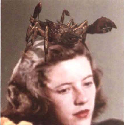
woman.##.tgafootage from the Project panel to the layer outline of the Timeline panel. LMB+drag thebug.##.tiffootage from the Project panel to the layer outline so that is sits on top of the newwoman.##.tgalayer. Scrub the timeline. The composite places a CG insect on top of the head of an actress (see Figure 4.29). Thewoman.##.tgafootage is taken from a digital copy of a public-domain instructional film. As such, there is heavy degradation in the form of MPEG compression artifacts, film grain, dust, and dirt. The CG, by comparison, is relatively clean. Aside from the lack of noise, the blacks found in the CG are significantly different from the blacks found in the live-action footage. To test this, move your mouse over the various areas and watch the RGB values change in the Info panel (see Figure 4.29). The darkest areas of the CG, such as the shadowed regions of the claws, have RGB values as light as 37, 28, 22. The darkest areas of the live-action footage, such as the region under the chin, have RGB values as dark as 13, 9, 0.To adjust the shadows, you can isolate and adjust the luminance information as well as change the overall color balance. Select the
bug.##.tiflayer in Comp 1, and choose Effect → Channel → Channel Combiner. In the Effect Controls panel, change the From menu to RGB To YUV. Select thewoman.##.tgalayer and choose Effect → Channel → Channel Combiner. In the Effect Controls panel, change the From menu to RGB To YUV. The viewer will display the composite in YUV space. To examine the Y luminance channel, change the Composition panel's Show Channel menu to Red (see Figure 4.30). Drag your mouse over the dark areas to compare the values in the Info panel. The darkest areas of the live-action footage have values around 24, 123, 134. The darkest areas of the CG have values around 47, 125, 130. Since the color space is YUV, this disparity between Y values represents a difference in luminance, or brightness. Note that the Channel Combiner effect may not display an accurate result in the viewer if a specific Working Space is chosen through the Project Settings dialog box. For example, if Working Space is set to HDTV (Rec. 709) instead of None, the output of the composition is altered by a Rec. 709 LUT before being sent to the monitor.Select the
bug.##.tiflayer in Comp 1 and choose Effect → Color Correction → Curves. In the Effect Controls panel, change the Curves effect's Channel menu to Red. The displayed curve controls the luminance. Insert points into the curve and adjust it to match Figure 4.31. This decreases the luminance of the darkest areas of the CG. Drag your mouse over the viewer and compare the values of the dark areas. The goal is to get the darkest areas of the CG to have values around 24, 123, 134.Once you're satisfied with the luminance adjustment, deselect the Fx button in the Effect Controls panel beside the Channel Combiner effect applied to the
woman.##.tgalayer. Select thebug.##.tgalayer and choose Effect → Channel → Channel Combiner. In the Effect Controls panel, change the From menu for the Channel Combiner 2 effect to YUV To RGB. Change the Composition panel's Show Channel menu to RGB. The viewer shows the composite in RGB space once again.Although the luminance values are a better match between the CG and the live-action blacks, the color balance is off. The live-action is heavily biased toward red, whereby the chin shadow produces values around 36, 15, 1. The tail of the insect, in comparison, has RGB values around 25, 20, 15. Select the
bug.##.tiflayer in the layer outline and choose Effect → Color Correction → Color Balance. In the Effect Controls panel, set Shadow Red Balance to 5, Shadow Green Balance to −5, Shadow Blue Balance to −10, Midtone Red Balance to 5, Midtone Green Balance to −5, and Blue Midtone Balance to −10.At this step, the CG has a higher color saturation than any part of the live-action. To match the washed-out quality of the footage, select the
bug.##.tiflayer in the layer outline and choose Effect → Color Correction → Hue/Saturation. In the Effect Controls panel, change the Master Saturation slider to −20. This results in more muted colors (see Figure 4.32).At this stage, the colors of the CG match the live-action fairly well. However, the CG does not possess the posterization or pixelization resulting from compression artifacts. You can emulate this with several specialized effects. Select the
bug.##.tiflayer in the layer outline and choose Effect → Stylize → Posterize. In the Effect Controls panel, change the Posterize effect's Level slider to 10. The effect limits the number of tonal steps in the layer, which causes color banding to occur.With the
bug.##.tiflayer selected in the layer outline, choose Edit → Duplicate. Select the newly createdbug.##.tiflayer (labeled 1 in the layer outline). Choose Effect → Stylize → Mosaic. In the Effect Controls panel, change the Mosaic effect's Horizontal Blocks and Vertical Blocks to 200. The effect reduces the number of visible pixels to 200 in each direction but does not shrink the layer (see Figure 4.33). To blend the pixelized version of the CG with the non-pixelized version, change the topbug.##.tiflayer's Opacity to 75%.Due to the blending of the two CG layers, the insect becomes darker. To offset this result, select the lowest
bug.##.tiflayer in the layer outline and choose Effect → Color Correction → Curves. In the Effect Controls panel, insert a new point in the Curves 2 effect's curve and shape the curve to match Figure 4.34. This lightens the insect body. To lighten the shadow, change the Curves 2 effect's Channel menu to Alpha. Insert a new point into the curve and shape it to match Figure 4.34. This darkens the mid-tone alpha values possessed by the cast shadow but does not unduly impact the higher alpha values of the insect body. Using the Render Queue, render a test movie. The tutorial is complete. A sample After Effects project is saved asae4.aepin the Tutorials folder on the DVD.


Matching CG elements can be a challenge, especially when the footage is not in pristine shape.
Create a new script. Choose edit → Project Settings. Change Frame Range to 1, 24 and Fps to 24. With the Full Size Format menu, choose New. In the New Format dialog box, change Full Size W to 720 and Full Size H to 540. Enter D1 into the Name field and click to the OK button.
In the Node Graph, RMB+click, choose Image → Read, and browse for the
bug.##.tifsequence in the Footage folder on the DVD. Select the Premultiplied check box in the Read1 properties panel. In the Node Graph, RMB+click, choose Image → Read, and browse for thewoman.##.tgasequence in the Footage folder on the DVD. Select the Read1 node, RMB+click, and choose Merge → Merge. Read1 is automatically connected to input A of the Merge1 node. Connect input B of Merge1 to Read2. Connect a viewer to the Merge1 node.The composite places a CG insect on top of the head of an actress (see Figure 4.35). The
woman.##.tgafootage is taken from a digital copy of a public-domain instructional film. As such, there is heavy degradation in the form of MPEG compression artifacts, film grain, dust, and dirt. The CG, by comparison, is relatively clean. Aside from the lack of noise, however, the blacks found in the CG are significantly different from the blacks found in the live-action footage. To test this, move your mouse over the various shadow areas and watch the RGB values change at the bottom of the Viewer pane. To switch the readout scale from the default HSVL (HSV/HSL) to 8-bit, change the viewer's Alternative Colorspace menu to 8bit (see Figure 4.35). The dark areas of the CG, such as regions near the claws, have RGB values as high as 52, 43, 34. The dark areas of the live-action, such as the shadow under the chin, have RGB values around 35, 15, 2.To aid in value adjustment, you can isolate the luminance information. Select the Merge1 node, RMB+click, and choose Color → Colorspace. In the Colorspace1 node's properties panel, change the leftmost Out menu from Linear to L*a*b*. Change the Viewer pane's Display_LUT menu to Linear. The viewer will display the composite in L*a*b* space. To examine the L* luminance channel, click the Viewer pane and press the R key (see Figure 4.36). You can also change the Display Style menu at the upper-left corner of the Viewer pane. Drag your mouse over the dark regions to compare the values. The CG has values around 89, 59, 56 in the dark regions while the live-action has values around 46, 40, 54. Since the readout represents L*, a*, and b* channels, the disparity between L* values represents a difference in luminance, or brightness.
Select the Read1 node, RMB+click, and choose Color → Grade. This inserts a Grade node between the Read1 node and the Merge1 node. In the Grade1 properties panel, change the Gamma slider to 0.7. The darkest areas of the CG gain values closer to 46, 40, 54.
Select the Colorspace1 node and change the Out menu from L*a*b* back to Linear. Change the Viewer pane's Display_LUT menu back to sRGB. Change the Display Style menu at the upper-left corner of the Viewer pane back to RGB. This effectively turns off the color space conversion. Although the luminance values are a better match between the CG and live-action, the color balance is off. Select the Grade1 node, RMB+click, and choose Color → ColorCorrect. In the ColorCorrect1 properties panel, change the Shadows Gain R cell to 1.4, the Shadows Gain B cell to 0.8, the Midtones Gain R cell to 1.4, and the Midtones Gain B cell to 0.8. To access the RGBA cells, click the 4 button to the right of sliders. The goal is to lower the CG RGB values to approximately 15, 7, 3 in the darkest areas, which is equivalent to the shadow values found around the actress's neck. (That is, you want the red channel to be twice as intense as the green channel and for there to be almost no blue.)
At this point, the CG has a higher color saturation than any part of the live-action. To match the slightly washed-out quality of the footage, change the ColorCorrect1's Master Saturation slider to 0.8 (see Figure 4.37).
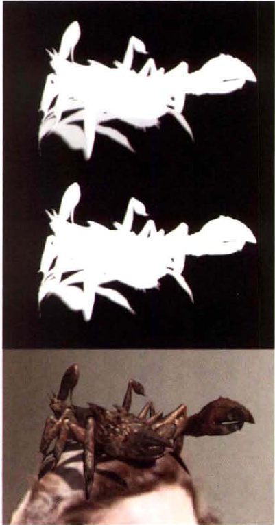
Although the dark areas of the CG are now similar to the dark areas of the live-action, the CG cast shadow remains too light. The cast shadow, in this case, is semitransparent, as is indicated by the gray pixels in the alpha channel. To view the alpha, connect a viewer to the ColorCorrect1 node, select the Viewer pane, and press the A key. To adjust the alpha, select the ColorCorrect1 node, RMB+click, and choose Color → ColorCorrect. In the ColorCorrect2 node's properties panel, change the Channels menu to Alpha. Change the Master Contrast slider to 1.12. This reduces the opacity and thus darkens the cast shadow (see Figure 4.38). The goal is have the cast shadows retain RGB values around 35, 19, 10, which more closely matches the dark areas of the hair.
At this stage, the blacks and overall shadow quality of the CG and live-action footage match fairly well (see Figure 4.38). However, a disparity remains between the posterization and pixelization of the live-action and the pristine quality of the CG. To solve this problem, you can use a Posterize node (Color → Posterize). However, the node tends to produce an output with a high contrast. In this situation, such contrast would interfere with the color balance of the CG and the opacity of its shadow. An alternative solution uses the built-in parameters of the Reformat node. With no nodes selected, RMB+click and choose Transform → Reformat. Disconnect the output of the ColorCorrect2 node from the Merge1 node. Instead, connect the output of ColorCorrect2 to the input of the Reformat1 node. Connect a viewer to Reformat1. Open the Reformat1 node's properties panel. Change the Type menu to To Box. Select the Force This Shape check box. Change the Width and Height cells to 144, 108. This will scale the input to 1/5 of the project's resolution (720 540). Change Filter to Impulse. The Impulse filter does not employ pixel averaging during the resize process and will thus create a limited-color, pixelized version of the CG. Change the Resize Type menu to Fit.
With the Reformat1 node selected, RMB+click and choose Transform → Transform. With the Transform1 node selected, RMB+click and choose Merge → Merge. Refer to Figure 4.39 as a reference. Connect the output of ColorCorrect2 to input B of Merge2. Connect the output of Merge2 to input A of Merge1. Connect a viewer to the output of Merge1 to see the result.
At this point, the pixelized CG bug is tucked into the bottom left corner of the composite. To fix this, open the Transform1 node's properties panel. Set the Scale slider to 5, the Translate X cell to 289, the Translate Y cell to 216, and the Filter menu to Impulse. The pixelized bug is placed on top of the unpixelized bug.
To reduce the intensity of the pixelization, reduce the Merge2 node's Mix slider to 0.3. (Mix is equivalent to opacity.) To soften the CG further, RMB+click over an empty area of the Node Graph and choose Filter → Blur. LMB+drag the Blur1 node and drop it on top of the connection line between the ColorCorrect2 and Merge2 nodes. The Blur1 node is inserted into the pipe. Change the Blur1 node's size to 1.5.
Render a test movie by disconnecting the Colorspace1 node from the network, selecting the Merge1 node, and choosing Render → Flipbook Selected from the menu bar. The tutorial is complete (see Figure 4.39). A sample Nuke script is included as
nuke4.nkin the Tutorials folder on the DVD.


Andy Davis attended the Art Center College of Design in Pasadena, California. After working as an illustrator for several years, he was able to apprentice under experienced compositors. He went on to freelance composite for such companies as Imaginary Forces, Asylum, and Big Red Pixel. He joined R!OT in 2006, where he served as a VFX supervisor. In 2009, R!OT merged with its sister company, Method Studios. Over the last 10 years, Andy has worked on commercials, PSAs, and over two dozen feature films including Gone in Sixty Seconds, Pearl Harbor, The League of Extraordinary Gentlemen, and Live Free or Die Hard.
Method Studios opened in 1998 and currently has offices in New York and Santa Monica. Method produces visual effects for commercials, music videos, and film. The studio has provided effects for such features as The Ring and the Pirates of the Caribbean series.

Andy Davis in his Inferno bay. The bay has a half dozen monitors.

The Method Studios facility in Santa Monica, California, a half-mile from the Pacific Ocean
(Method Studios currently uses as a combination of Inferno, Nuke, and Shake for compositing. The Santa Monica studio has over a dozen compositors on staff but expands for large projects.)
LL: Is it still common to work with 35mm footage?
AD: 35mm is still standard. We have quite a lot of Red [HD footage] coming through here nowadays, both for DI and for some commercials, but I think that's going to become more and more the case. The problem is that [HD footage] takes a huge amount of disk space. People make the wrong assumption that just because there's no film processing doesn't mean that it won't need to be converted to DPXs or something [similar]....
LL: What are the main differences between 35mm and high-definition video?
AD: Color depth for one.... The color range is definitely better in film than it is in digital.... The contrast between the lights and the shadows are [more easily] captured on film. I'd say also that most cinematographers are schooled on 35mm. The guys who are the best computer technicians aren't necessarily the best DPs (directors of photography) out there. And everyone seems to understand 35mm. It's pretty much a standard. I'm not really afraid of 35mm going away anytime soon.
LL: What are some advantages of digital video?
AD: What it does is give people the option to shoot [more footage]. With the new cameras [that are being developed], the concept of being able to shoot an IMAX-resolution film on a Steadicam is crazy. Traditional IMAX cameras are gigantic, and all you normally see is boring movies about beavers.... [Digital video camera makers] are really trying to push the envelope. If it wasn't for Red, the Panavisions of the world wouldn't be pushing [the technology]. That said, it isn't perfect. The progressive shutter is a problem for fast movement.... If you're comparing [35mm] to the Red, the Red at least can do 4K, whereas, if you need a hi-res scan of 35mm, the film grain can be a little big.
LL: How important is color grading?
AD: Color is the basis of it all. Color can make or break anything. I really keep an eye out for guys with [a good sense of color]. It's even more critical with film because you have to anticipate what it's going to look like after it goes through the film process.... If the blacks are off a bit, you'll notice it on a 50-foot screen.
LL: How important have DI (digital intermediates) become?
AD: DI is really going to change telecine. The thing that made telecine so handy is that it's fast and interactive. Clients loved being able to walk out with a tape in their hand. DI, however, does give you the ability to be more articulate with mattes.... [DI] just opens up a whole bunch of possibilities.
LL: Do you take any special steps for color grading?
AD: We use 3D LUTs and 2D monitor LUTs. More often than not, when I'm working on film I'll be using monitor LUTs. I'd rather trick the monitor into giving me the right information rather than doing log to lins (logarithmic to linear conversions) and lins to logs all the time.
