Color is not contained within the materials of objects. Instead, color is the result of particular wavelengths of light reaching the viewer through reflection or transmission. Different materials (wood, stone, metal, and so on) have different atomic compositions and thereby absorb, reflect, and transmit light differently. This natural system is therefore considered a subtractive color system. When a wavelength of light is absorbed by a material, it is thus subtracted from white light, which is the net sum of all visible wavelengths. Hence, the red of a red object represents a particular wavelength that is not absorbed but is reflected or transmitted toward the viewer.

RYB and RGB Color Models

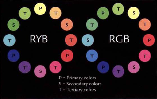
When discussing color in the realm of fine arts, color models are invoked. Color models establish primary colors, combinations of which form all other visible colors. The red-yellow-blue (RYB) color model, used extensively for nondigital arts, traces its roots back to eighteenth-century color materialism, which assumes that primary colors are based on specific, indivisible material pigments found in minerals or other natural substances. The popularization of specific RYB colors was aided by printmakers of the period who employed the color separation printing process.

The development of computer graphics, however, necessitated a new color model with a new set of primary colors: red, green, and blue, commonly known as RGB. Through an additive process, computer monitors mix red, green, and blue light to produce additional colors. Added in equal proportions, RGB primaries produce white. In contrast, the RYB color model is subtractive in that the absence of red, yellow, and blue produces white (assuming that the blank paper or canvas is white). Modern printing techniques follow the subtractive model by utilizing cyan, magenta, and yellow primary inks, with the addition of black ink (CMYK, where K is black). The RGB color model is based upon mid-nineteenth-century trichromatic color theories, which recognized that color vision is reliant on unique photoreceptor cells that are specifically tuned to particular wavelengths.

Both the RYB and RGB models are often displayed as color wheels (see Figure 2.1). Despite the difference between the RYB and RGB models, artistic methods of utilizing an RYB color wheel are equally applicable to an RGB color wheel.

Figure 2.1. RYB and RGB color wheels. Secondary colors are mixtures of two primary colors. Tertiary colors are mixtures of a primary and a secondary color. An RGB version of this figure is included as colorwheel.tif in the Footage folder on the DVD.

Employing Color Harmony

The goal of color selection is color harmony, which is the pleasing selection and arrangement of colors within a piece of art. The most common methods of choosing harmonic colors from a color wheel are listed here:

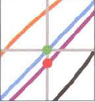
• Complimentary Colors. A pair of colors at opposite ends of the color wheel. With an RGB color wheel, blue and yellow are complimentary colors (see the left image of Figure 2.2).

• Split Compliment One color plus the two colors that flank that color's complimentary color. With an RGB color wheel, green, blue-violet (purple), and red-violet (pink) form split compliments (see the right image of Figure 2.2).

• Analogous Colors Colors that are side by side (see the left image of Figure 2.3). With an RGB color wheel, yellow and orange are analogous.

• Diad Two colors that have a single color position between them (see the right image of Figure 2.3). With an RGB color wheel, cyan and green form a diad. Along those lines, a triad consists of three colors that are equally spaced on the wheel (such as red, green, and blue).

Figure 2.2. (Left) Complimentary blue and yellow patterns appear on an angelfish. (Right) Green, blue-violet, and red-violet light in a broadcast graphic create a split compliment. (Images © 2009 by Jupiterimages).

Figure 2.3. (Left) The yellow and orange of an abstract digital painting function as analogous colors. (Right) the green of limes and the cyan of a glass bowl form a diad. (Images © 2009 by Jupiterimages)

Gamut represents all the colors that a device can produce. Color space refers to a gamut that utilizes a particular color model. (For example, sRGB and Rec. 709 are color spaces, while RYB and RGB are color models.) The color space available to various output devices varies greatly. For example, the color space that a high-definition television can output is significantly different from the color space available to a computer monitor or an ink-jet printer. The variations in color space necessitate the calibration of equipment to ensure correct results when it comes to color reproduction. As a compositor, you should know if your own monitor has been calibrated. In addition, it's important to know what type of color grading will be applied to your work. Color grading is the process by which the colors of the footage are adjusted or enhanced in anticipation of its projection on film, broadcast on television, display on the Internet, or inclusion in a video game. (Prior to digital technology, the motion picture grading process was known color timing.)

Working with Gamma

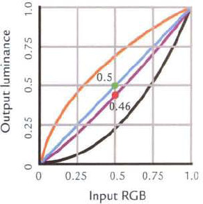
Computer monitors operate in a nonlinear fashion. That is, the transition from darks to lights forms as a delayed curve (see Figure 2.4). With a CRT (Cathode Ray Tube) monitor, this curve results from the nonlinear relationship between the grid voltage (voltage applied to the electron gun) and luminance (the net effect of electrons shot at the screen's phosphors). Mathematically, the curve is shaped by gamma, which is the exponent of a power function. That is, the voltage of the gun must be raised by the power of gamma for an equivalent raise in the screen's luminance. When discussing the specific gamma of a particular monitor, the term native gamma is used. Liquid Crystal Display (LCD) and plasma screens do not employ electron guns; however, they do apply varying amounts of voltage to liquid crystals or plasma electrodes. As such, LCD and plasma screens exhibit gamma curves similar to CRTs.

Figure 2.4. The uncalibrated gamma curve of a mid-priced LCD monitor. Note that the red, green, and blue channels each have a slightly different response. The graph has been normalized to a range of 0 to 1.0.

If there is no compensation for a monitor's native gamma, the digital image will gain additional contrast through its mid-tones and may lose detail in the shadows or similarly dark areas (see Figure 2.5).

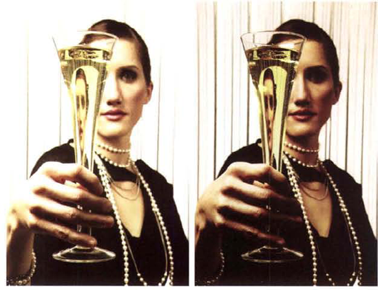
Figure 2.5. (Left) A digital photo with gamma correction applied. (Right) Same photo without gamma correction. The contrast is exaggerated for print. (Photos © 2009 by Jupiterimages).

Industry Perspective: LCDs vs. CRTs

LCD and plasma screens are rapidly replacing CRTs in the professional world of animation and visual effects. Unfortunately, this has led to additional calibration difficulties. LCD screens have a viewing angle that is narrower than a CRT. Thus, the effect of a display gamma curve is subject to how off-center the viewer is as he or she sits or stands. In addition, LCDs have a poor record when it comes to color accuracy and consistency. "Color critical" LCD monitors have been available to studios for a number of years, but their high price tag has made them impractical when outfitting a large number for seats for animators or compositors. This situation has led some studios to stockpile CRT monitors in anticipation of their disappearance. Fortunately, recent advances in technology have begun to address this issue. For example, the moderately priced Hewlett-Packard DreamColor LCD monitor, codeveloped by DreamWorks Animation, offers a 30-bit color space (10-bits per channel), hardware support for industry-standard color profiles, and an LED backlight that produces a contrast range of 1000:1.

To avoid this, operating systems apply gamma correction. Gamma correction is the inverse power function of the monitor's native gamma. That is, gamma correction creates a curve which neutralizes the monitor's native gamma curve, thus making the monitor's response roughly linear. The gamma correction curve is defined by a single number. With Windows operating systems, the default is 2.2. With Macintosh OS-X, the default is 1.8. Ideally, gamma correction would adjust the pixel values so that their displayed luminance corresponds to their original values. However, since native gamma curves generally don't match the gamma correction curves, this becomes difficult. For example, the average CRT monitor carries a native gamma of 2.5. Hence the resulting system or end-to-end gamma on a Windows system is 1.14, which equates to 2.5 / 2.2. In other words, a pixel with a value of 0.5 ultimately receives an adjusted value of 0.46 (see Figure 2.6). Thus, the gamma correction formula can be written like this:

new pixel value = pixel value(native gamma / gamma correction)

Figure 2.6. Pixel value curve (cyan), native gamma curve (black), gamma correction curve (orange), and final adjusted curve (violet). The green dot indicates the original pixel value of 0.5. The red dot indicates the final adjusted pixel value of 0.46.

Standard digital images carry three channels: one for red, one for green, and one for blue. (An optional fourth channel, alpha, is discussed in Chapter 3, "Interpreting Alpha and Creating Mattes.") The bit depth of each channel establishes the number of tonal steps that are available to it. Each tonal step is capable of carrying a unique color value. The term bit depth refers to the number of assigned bits. A bit is a discreet unit that represents data in a digital environment. (A byte, in contrast, is a sequence of bits used to represent more complex data, such as a letter of the alphabet.)

When bit depth is expressed as a number, such as 1-bit, the number signifies an exponent. For example, 1-bit translates to 2¹, equaling two possible tonal steps for a single channel of any given pixel. Other common bit depths are listed in Table 1.1. When discussing bit depth, tonal steps are commonly referred to as colors.

Bit depth is often expressed as bpc, or bits per channel. For example, an RGB image may be labeled 8-bpc, which implies that a total of 24 bits is available when all three channels are utilized. The 2 used as a base in each Table 1.1 calculation is derived from the fact that a single bit has two possible states: 1 or 0 (or true/false or on/off).

When discussing bit depth, specific ranges are invoked. For example, an 8-bit image has a tonal range of 0 to 255, which equates to 256 tonal steps. A 15-bit image has a tonal range of 0 to 32,767, which equates to 32,768 tonal steps. To make the application of bit depth more manageable, however, the ranges are often normalized so that they run from 0 to 1.0. In terms of resulting RGB color values, 0 is black, 1.0 is white, and 0.5 is median gray. Regardless, an 8-bit image with a normalized range continues to carry 256 tonal steps, and a 15-bit image with a normalized range carries 32,768 tonal steps. The tonal steps of an 8-bit image are thus larger than the tonal steps for a 15-bit image. For example, the darkest color available to an 8-bit image, other than 0 black, is 0.004 on a 0 to 1.0 scale. The darkest color available to a 15-bit image is 0.00003 on a 0 to 1.0 scale. (Note that normalized ranges are used throughout this book in order to simplify the accompanying math.)

Two bit depth variants that do not possess such limited tonal ranges are 16-bit floating point (half float) and 32-bit floating point (float). Due to their unique architecture, they are discussed in the section "Integer vs. Float" later in this chapter.

When it comes to bit depth, there is no universally accepted standard at animation studios, visual effects houses, and commercial production facilities. Although full 32-bit float pipelines have become more common in the last several years, it's not unusual to find professional animators and compositors continuing to work with 8-, 10-, 12-, 15-, or 16-bit formats with linear, log, integer, and float variations. In fact, a single project will often involve multiple formats, as there are specific benefits for using each. Hence, one troublesome aspect of compositing is back-and-forth conversions.

Converting a low-bit-depth image to a high-bit-depth image does not degrade the image. However, such a conversion will create a combed histogram (see Figure 2.8). A histogram is a graph that displays the number of pixels found at each tonal step of an image. (For more detail on histograms, see Chapter 4.) The combing is a result of a program distributing a limited number of tonal steps in a color space that has a greater number of tonal steps. Visually, this may not affect the image since the gaps in the comb may be as small as one tonal step. However, if successive filters are applied to the converted image, quality may be degraded due to the missing steps. When the gaps grow too large, they result in posterization (color banding).

Figure 2.8. (Left) 8-bit image converted to 16 bits (Top Right) The image's combed blue-channel histogram (Bottom Right) The same histogram after repair

There's no automatic solution for repairing the combing. However, there are several approaches you can take:

Converting a high-bit-depth image to a low-bit-depth image is equally problematic because information is lost. Either superwhite values (values above the low bit-depth's maximum allowable value) are thrown away through clipping or other value regions are lost through tone mapping. Tone mapping, the process of mapping one set of colors to a second set, is demonstrated in Chapter 12, "Advanced Techniques."

Compositing packages, such as After Effects and Nuke, offer built-in solutions that make managing multi-bit-depth projects somewhat easier. These solutions are discussed and demonstrated at the end of this chapter.

As light photons strike undeveloped film stock, the embedded silver halide crystals turn opaque. The greater the number of photons, the more opaque the otherwise transparent stock becomes. The "opaqueness" is measured as optical density. The interaction between the photons and the stock is referred to as exposure. The relationship between the density and exposure is not linear, however. Instead, the film stock shows little differentiation in its response to low-exposure levels. At the same time, the film stock shows little differentiation in its response to high-exposure levels. This reaction is often represented by film characteristic curve graphs (see Figure 2.9).

The typical characteristic curve for film includes a toe and a shoulder. The toe is a flattened section of curve where there is little response to low-exposure levels. The shoulder is a semi-flattened section of curve where there is a slowed response to high levels of exposure. Ultimately, the reduced response in these two areas translates to a reduced level of contrast in the film. Hence, cinematographers are careful to expose film so as to take advantage of the characteristic curve's center slope. This exposure range produces the greatest amount of contrast in the recorded image, and it is referred to as the film's latitude.

Characteristic curves are logarithmic. With each equal step of a logarithm, the logarithmic value is multiplied by an equal constant. For example, in Figure 2.9 the log is in base 10. Hence, each step is 10 times greater (or less) than the neighboring step. For example, the exposure level, as measured in lux seconds, is mapped to the x-axis. (A lux is an international unit for luminous emittance, and it is equivalent to one candela source one meter away; a candela is roughly equivalent to an average candle.)

Figure 2.9. A generic film characteristic curve

The values run from −1.0 to 2.0. On the logarithmic scale, −1.0 equates to 10⁻¹, or 0.1; 0 equates to 10⁰, or 1.0; and 2.0 equates to 10², or 100. Hence, the x-axis indicates a range in from 1/10 of a second to 100 seconds. At 1/10 of a second, the film is exposed to 1/10 of a lux. At 100 seconds, the film is exposed to 100 lux. The x-axis of characteristic curves can also be assigned to generic relative exposure units or f-stops. The y-axis is assigned to the optical density and is also measured on a logarithmic scale. A value of 3 marks the maximum "opaqueness" achievable by the film stock.

Log File Formats

To take advantage of film's nonlinear nature, several image formats offer logarithmic (log) encoding. These include DPX and Cineon (which are detailed in the section "Favored Image Formats" later in this chapter). Although the formats can reproduce the film fairly accurately, they are difficult to work with. Most digital imaging, visual effects, and animation pipelines, whether at a studio or through a specific piece of software, operate in linear color spaces. Hence, it is common to convert log files to linear files and vice versa. The difficulty lies in the way in which log and linear files store their data.

Linear files store data in equal increments. That is, each tonal step has equal weight regardless of the exposure range it may be representing. For example, with 8-bit linear color space, doubling the intensity of a pixel requires multiplying a value by 2. You can write out the progression as 1, 2, 4, 8, 16, 32, and so on. As the intensity doubles, so does the number of tonal steps required. Each doubling of intensity is equivalent to an increase in stop. (Stop denotes a doubling or halving of intensity, but does not use specific f-stop notation, such as 1.4 or 5.6.) Hence, each stop receives a different number of tonal steps. The disparity between low and high stops becomes significant. For example, the lowest stop has 1 tonal step (2 – 1), while the highest stop has 128 steps (256 – 128). In contrast, 8-bit log color space only requires an incremental increase in its exponent to double the intensity. The logarithmic formula is written as logb(x) = y, where_b is the base and y is the exponent. For example, the log base 10 of 100 is 2, or log₁₀(100) = 2; this equates to 10² = 100. If log base 10 has an exponent progression that runs 0, 0.5, 1.0, 1.5, 2, the logarithmic values are 1, 3.16, 10, 31.62, 100. In this case, each logarithmic value represents a stop. If the logarithmic values are remapped to the 0 to 256 8-bit range, those same stops earn regularly-spaced values (0, 64, 128, 192, 256). As such, each of the four stops receive 64 tonal steps. If you restrict the linear color space to four stops, the progression becomes 32, 64, 128, 256. When the 4-stop linear color space is placed beside the 4-stop logarithmic color space, the uneven distribution of tonal steps becomes apparent(see Figure 2.10).

Figure 2.10. Eight compositing steps used by Freestyle Collec 4-stop, 8-bit log and 4-stop, 8-bit linear color ranges. Note how each stop has a dissimilar number of tonal steps. Each stop captures twice the amount of light, or is twice as intense, as the stop below it.

Common image formats, such as JPEG or Targa, store integer values. Since an integer does not carry any decimal information, accuracy is sacrificed. For example, if you snap a picture with a digital camera and store the picture as a JPEG, a particular pixel may be assigned a value of 98 even though a more accurate value would be 98.6573. Although such accuracy is not critical for a family photo, it can easily affect the quality of a professional composite that employs any type of filter or matte.

Floating-point image formats solve the problem of accuracy by allowing for decimal values. When a value is encoded, the format takes a fractional number (the mantissa) and multiplies it by a power of 10 (the exponent). For example, a floating-point number may be expressed as 5.987e+8, where e+8 is the same as ×10⁸. In other words, 5.987 is multiplied by 10⁸, or 100,000,000, to produce 598,700,000. If the exponent has a negative sign, such as e–8, the decimal travels in the opposite direction and produces 0.00000005987 (e−8 is the same as × 10⁻⁸). Additionally, floating points can store either positive or negative numbers by flipping a sign bit from 0 to 1.

Floating-point formats exist in two flavors: half float and float. Half float (also known as half precision) is based on 16-bit architecture that was specifically developed for the OpenEXR format. Half float file sizes are significantly smaller than 32-bit float files. Nevertheless, OpenEXR half float supports dynamic ranges as large as 30 stops.

Aside from decimal accuracy, float formats offer the following advantages:

Despite the capacity for a monstrous dynamic range, float formats remain linear and are thus not as accurate as log formats when film is encoded.

Digital image formats support various bit depths and fall into two major categories: linear and log (logarithmic). Within these two categories, there are two means in which to store the data: integer and float (floating point). If a format is not identified as float, then it operates on an integer basis. Here is a partial list of image formats commonly favored in the world of compositing:

After Effects and Nuke support a wide range of bit depths. In addition, they are able to simulate color spaces commonly encountered in the professional world of compositing.

Working in AE

Recent versions of After Effects support 8-bit integer, 16-bit integer, and 32-bit float projects. To select the bit depth, choose File → Project Settings. In the Project Settings dialog box, change the Depth menu to 8 Bits Per Channel, 16 Bits Per Channel, or 32 Bits Per Channel (Float). If lower-bit-depth footage is imported into a higher-bit-depth project, After Effects automatically upconverts the footage. Note that Adobe's 16-bit space is actually a 15-bit color space with one extra step.

Color Management in AE

By default, After Effects does not apply any type of color management. That is, no special color profiles are applied to any input or output. However, if the Working Space menu is switched from None to a specific color profile in the Project Settings dialog box, the following occurs:

1. Each piece of imported footage is converted to the working color space as defined by the Working Space menu. The native color space of the footage is either retrieved from its file as an embedded ICC profile or defined by the user in the Interpret Footage dialog box (see the section "AE Tutorial 2: Working with DPX and Cineon Files" later in this chapter).

2. After Effects performs all its color operations in the working color space.

3. To display the result on the screen, After Effects converts the images to system color space via a LUT generated by the monitor profile (which is carried by the computer's operating system).

4. When rendered through the Render Queue, the images are converted to output color space, which is defined by the Output Profile menu of the Color Management tab in the Output Module Settings dialog box.

Common Color Profiles

After Effects offers a long list of profiles through its Working Space menu, including the following:

• sRGB IEC6 1966-2.1 The sRGB IEC6 1966-2.1 profile is an RGB color space developed by Hewlett-Packard and Microsoft. Since its inception in the mid-1990s, it has become an international standard for computer monitors, scanners, printers, digital cameras, and the Internet. The IEC6 1966-2.1 component refers to an official specification laid down by the International Electrotechnical Commission (IEC).

• HDTV (Rec. 709) As its name implies, HDTV (Rec. 709) is the standard color space for high-definition television. The Rec. 709 component refers to a specific recommendation of the International Telecommunication Union (ITU).

• SMPTE-C The SMPTE-C profile is the standard color space for analog television broadcast in the U.S. The space was standardized by the Society of Motion Picture and Television Engineers in 1979.

• SDTV NTSC and SDTV PAL The SDTV NTSC and SDTV PAL profiles are the color spaces for standard-definition video cameras. The profiles use the same tonal response curves as HDTV (Rec. 709).

Tips & Tricks: 16-235 Profiles

Several profiles, including SDTV NTSC, SDTV PAL, and HDTV (Rec. 709), have a variant with 16-235 as a suffix. The 16-235 profiles are designed to maintain proper luma levels when you import and export video. When video is captured, the image values are represented by voltages measured as mV (millivolts) or IRE (a unit developed by the Institute of Radio Engineers). When the voltages are converted to Y'CbCr (a video color space with luma, blue chroma, and red chroma components), the voltage values are often fixed to an 8-bit range of 16 to 235. (With NTSC video, values under 16 and over 235 are considered to be "unsafe.") Hence, After Effects offers 16-235 profiles to maintain or compress the luma range. If a 16-235 profile is selected through the Working Space menu of the Project Settings dialog box and the Assign Profile menu of the Interpret Footage dialog box, the 16-235 luma range is maintained. If a 16-235 profile is selected for the Output Profile menu but the Working Space menu is set to a non-16-235 profile, the luma range is compressed at the point of render. For a definition of luma, which varies from luminance, see Chapter 4, "Channel Manipulation."

Color Profile Converter

In addition to the Working Space menu, After Effects provides a Color Profile Converter effect (Effect → Utility → Color Profile Converter). With the effect, you can choose an input profile and an output profile for the layer to which it's applied. The style of the conversion is controlled by the Intent menu. The Perception property attempts to maintain the visual consistency of colors between color spaces. The Saturation option preserves high saturation values at the expense of color accuracy. Relative Colorimetric remaps values from one color space to the next. Absolute Colorimetric does not alter values but instead clips any colors that fall outside of the range of the new color space. The Color Profile Converter should not be used in conjunction with color management, however, as errors may occur. If the effect is used, the Working Space menu in the Project Settings dialog box should be set to None.

Linearization

In After Effects, it's possible to switch from a gamma-corrected color space to a non-corrected color space. Within a non-corrected color space, no gamma curve is applied and values are not altered in anticipation of display on a monitor. There are two methods with which to apply the conversion. In the Project Settings dialog box, you can select a profile through the Working Space menu and then select the Linearize Working Space check box. This linearizes the entire project. Otherwise, you can leave Working Space set to None and select the Blend Color Using 1.0 Gamma check box. In certain situations, a linearized space offers greater accuracy when blending layers together.

Color Space Simulation

If you've chosen a profile through the Working Space menu, you can simulate a color space other than sRGB through the viewer. For example, you can simulate an NTSC video output on your computer monitor even though the monitor has a color space inherently different than a television. To select a simulation mode, choose View → Simulate Output → Simulation Mode. You can create a custom simulation mode by choosing View → Simulate Output → Custom. The process occurs in four steps in the Custom Simulation Output dialog box (see Figure 2.11):

1. In the first step, the imported image is converted using the Working Space profile. This profile is listed at the top of the dialog box as the Project Working Space.

2. In the second step, the resulting image is converted using the output profile. Although the menu defaults to Working Space, you have a long list of optional profiles. Special profiles provided by Adobe include those that emulate specific 35mm motion picture film stocks and specific makes of HD digital video cameras. Note that this Output Profile option operates independently of the one found in the Color Management tab of the Output Module Settings dialog box.

3. In the third step, the resulting image is converted using the simulation profile. The conversion preserves the color appearance of the image within the color limits of the simulated device, but not the numeric color values. If the Preserve RGB check box is selected, however, the opposite occurs, whereby the color values are maintained at cost to the visual appearance. Preserve RGB may be useful when working exclusively with film stock. In either case, the simulation does not affect the way in which the image is rendered through the Render Queue.

4. As a final step, the resulting image is converted to the monitor profile provided by the computer's operating system so that it can be displayed on the screen.

Figure 2.11. Custom Output Simulation dialog box

Log-to-Linear Conversions in AE

After Effects provides a means by which to convert log images to linear through the Project panel. To do so, follow these steps:

1. In the Project panel, RMB+click over the log file name and choose Interpret Footage → Main. In the Interpret Footage dialog box, switch to the Color Management tab and click the Cineon Settings button. The Cineon Settings dialog box opens. The 10 Bit Black Point cell represents the value within the log file that is converted to the Converted Black Point value. The 10 Bit White Point cell represents the value within the log file that is converted to the Converted White Point value. The Gamma cell establishes the gamma curve applied to the log file to prepare it for viewing. You can enter values into the cells or choose one of the options through the Preset menu. (For information on black and white points, see the section "Log vs. Linear" earlier in this chapter.)

2. When you change Preset to Video, the program undertakes a conversion that is designed for video. With this setting, the Converted Black Point cell is set to 16 and the Converted White Point cell is set to 235. This is equivalent to the broadcast-safe 16 to 235 range for Y'CbCr color space.

3. If you change the Preset menu to Custom, you can enter your own values. This may be necessary when preparing digital sequences for film out (recording to motion picture film) at a lab that requires specific black and white points. Changing the Units menu to 8-bpc or 16-bpc affects the way the various values are displayed in the dialog box; however, the conversion continues to happen in the current bit depth of the project.

4. To retrieve lost highlights, raise the Highlight Rolloff cell. This crushes the upper range so that the highest output values are no longer at the bit-depth limit. For example, a Highlight Rolloff value of 20 prevents any value from surpassing 29,041 in After Effects 16-bit color space.

A second approach to working with log files involves the use of the Cineon Converter effect. To apply the effect, follow these steps:

1. Select the log file or log footage in the layer outline of the Timeline tab. Choose Effect → Utility → Cineon Converter. The Cineon image will instantly gain contrast in the viewer.

2. To adjust the overall contrast within the image, change the Black Point and White Point sliders. The sliders are divided into two groups: 10 Bit and Internal. The 10 Bit sliders function in the same manner as the 10 Bit sliders found in the Cineon Settings dialog box. The Internal sliders function in the same manner as the Converted sliders found in the Cineon Settings dialog box. The Highlight Rolloff and Gamma properties are also identical. Note that Conversion Type is set to Log To Linear.

Tips & Tricks: 10-Bit Log Files

By default, when the Preset menu in the Cineon Settings dialog box is changed to Standard, Video, or Over Range, the 10 Bit Black Point cell is set to 95 and the 10 Bit White Point cell is set to 685. This represents the acceptable motion picture film exposures of 10 percent and 90 percent reflective cards. For more information, see the "Log vs. Linear" section earlier in this chapter.

If you need to render 10-bit log files, you can open the Output Module Settings dialog box through the Render Queue tab. In the dialog box, change the Format menu to Cineon Sequence, switch to the Color Management tab, click the Cineon Settings button, and change the Preset menu to Full Range. Note that the Gamma property is automatically returned to 1.0. You can choose between FIDO/Cineon 4.5 or DPX flavors by selecting one of the File Format radio buttons.

Working in Nuke

Nuke is based on linear 32-bit floating-point architecture. All operations occur in linear 32-bit floating-point space. When lower-bit-depth images are imported into the program, they are upconverted to 32-bpc. Whether or not the incoming data is interpreted as linear or log, however, is determined by the Colorspace menu of the Read node (see Figure 2.12).

Figure 2.12. The Colorspace menu in the properties panel of a Read node

Color Space in Nuke

Each color space accessible through a Read node is emulated by a LUT provided by Nuke. The following spaces are available:

• Linear has no affect on the input pixels. On a normalized scale, 0 remains 0, 0.5 remains 0.5, and 1 remains 1.

• sRGB is the standard sRGB IEC6 1966-2.1 color space.

• rec709 is the standard HDTV color space. Both sRGB and rec709 use a gamma curve.

• Cineon is a 10-bit log color space. If the Colorspace menu is set to Cineon, the Read node converts the log file to linear space using conversion settings recommended by Kodak, author of the Cineon format. To override the conversion, you can select the Raw Data check box. In this case, the Colorspace parameter is disabled. You are then free to connect a Log2Lin node to the Read node (see the next section).

• Default is a color space determined by the script's Project Settings properties panel. Nuke allows the user to select default color space LUTs for various imported/exported file formats and interface components. For example, an sRGB LUT is automatically assigned to the default viewer. Hence, images sent to a viewer are first processed by the sRGB LUT.

You can view the current script's LUT settings by choosing Edit → Project Settings and switching to the LUT tab of the properties panel. The default LUT settings are listed at the bottom. You can change any listed inputs/outputs to a new LUT by selecting a LUT from the corresponding pull-down menu. If you click on a LUT listed at the top left, the LUT curve is displayed in the integrated curve editor (see Figure 2.13).

Figure 2.13. The LUT tab curve editor with the sRGB LUT displayed

In the editor, the x-axis represents the input pixel values and the y-axis represents the output pixel values (normalized to run from 0 to 1.0). You can create a new LUT by clicking the small + button at the bottom of the LUT list and entering a name into the New Curve Name dialog box. The new LUT curve is displayed in the curve editor and is linear by default. You can manipulate the shape of the curve by inserting and moving points. To insert a new point, select the curve so that it turns yellow and Ctrl+Alt+click on the curve. To move a point, LMB+drag the point. In addition, you can LMB+drag the resulting tangent handles. To reset the curve to its default linear shape, click the Reset button at the bottom of the LUT list.

Log-to-Linear Conversions in Nuke

Nuke offers a node with which to convert a log input to a linear output. To apply the node, follow these steps:

1. Select the node you wish to convert from a log space to a linear space. If the node is a Read node, make sure that the Raw Data check box is selected in the Read node's properties panel. In the Node Graph, RMB+click and choose Color → Log2Lin. Open the Log2Lin node's properties panel.

2. The Black parameter establishes the black point (the value within the log file that will be converted to 0 value within the current 32-bit linear color space). The White parameter establishes the white point (the value within the log file that will be converted to a maximum value within the current 32-bit linear color space). The Gamma parameter defines the gamma correction curve that is applied to the output in anticipation of its display on the monitor.

Color Space Tutorials

Discussions of color space, color profiles, and simulation modes can be confusing. Therefore, it's often easier to think of specific scenarios that may be encountered in the professional world.

AE Tutorial 2: Working with DPX and Cineon Files

You may be tasked to composite a shot that involves effects and greenscreen footage. Ideally, the footage would be digitized using a single image format at a consistent bit depth. However, the reality is that multiple formats and bit depths are usually employed. This is due to the varied technical limitations of camera equipment, the distribution of work to different production units or companies who have different working methodologies, and the fact that different formats and bit depths are better suited for specific shooting scenarios. Regardless, you will need to convert all incoming footage to an image format and bit depth that is suitable for the project to which the composite belongs.

More specifically, you may be faced with the following situation. Greenscreen footage is shot on 35mm and is provided to you as 10-bit log Cineon files. Effects footage, shot several years earlier, is culled from the studio's offline shot library; 10-bit log DPX is the only format available. Background plate footage is shot with an HD digital video camera; the 12-bit linear TIFF files are converted to 16-bit before they are handed to you. Your composite is part of a visual effects job for a television commercial. Due to budget considerations, the clients have decided to deliver the project as standard definition (SD). Your shot will be passed on to a Flame bay for color grading. Nevertheless, you will need to have your work approved by your supervisor. You're using a CRT monitor to judge your work. Although the monitor is calibrated, it can only approximate the look of an SDTV system.

In light of such a situation, you can take the following steps in After Effects when setting up a new composite:

1. Create a new project. Choose File → Project Settings. In the Project Settings dialog box, set Depth to 16 Bits Per Channel. 16-bit depth is necessary to take advantage of the 10-bit DPX, 10-bit Cineon, and 16-bit TIFF footage that will be imported. Although the ultimate project output will be 8-bit images for SDTV, it's best to work in a higher bit depth until the final render. Set the Working Space menu to SDTV NTSC. It's also best to work within the color space utilized by the final output. Select the Frames radio button (see Figure 2.14).

2. Choose Composition → New Composition. In the Composition Settings dialog box, set the Preset menu to NTSC D1 Square Pixel, the Frame Rate to 30, and Duration to 30, and click OK. Choose View → Simulate Output → SDTV NTSC. Henceforth, the viewer will simulate SDTV broadcast color space.

3. Choose File → Import → File. Browse for the bg_plate.tif file in the Footage folder on the DVD (see Figure 2.15).

   

   Figure 2.14. The top of the Project Settings dialog box

4. Choose File → Import → File. Browse for the greenscreen.cin file in the Footage folder on the DVD. RMB+click over the greenscreen.cin filename in the Project panel and choose Interpret Footage → Main. In the Interpret Footage dialog box, switch to the Color Management tab. Note that the Assign Profile menu is automatically assigned to Working Space - SDTV NTSC. Since the footage was not shot in an SDTV format, check the Preserve RGB check box to avoid color filtering. Despite this setting, the image appears washed out in the simulated SDTV NTSC color space of the viewer (see Figure 2.15).

   

   Figure 2.15. (Left) Background plate (Right) Unaltered greenscreen file. Since the file is a 10-bit log Cineon, it appears washed out in the simulated SDTV NTSC color space of the viewer.

5. To restore contrast to the greenscreen, click the Cineon Settings button in the Interpret Footage dialog box. In the Cineon Settings dialog box, change the Preset menu to Standard (see Figure 2.16). When you choose Standard, the program undertakes a conversion that expands the log file's 95 to 685 tonal range to a 0 to 32,768 project tonal range. For more information on the conversion process, see the section "Log-to-Linear Conversions in AE" earlier in this chapter.

6. Choose File → Import → File. Browse for the effect.##.dpx sequence in the Footage folder on the DVD. Through the Interpret Footage dialog box, select the Preserve RGB check box and match the Cineon settings of the greenscreen.cin file.

   

   Figure 2.16. Log-to-linear conversion is carried out by the Standard preset in the Cineon Settings dialog box.

   Tips & Tricks: Film and Video Profiles

   The Assign Profile menu of the Interpret Footage dialog box includes a list of specific motion picture film stocks and digital video camera formats. The profiles are designed to match the characteristic curves of the stocks and formats. Providing an exact profile match is desirable when possible.

7. To assemble the composite, LMB+drag bg_plate.tif from the Project panel into the layer outline of the Timeline panel. LMB+drag the effect.##.dpx footage on top of the new bg_plate.tif layer. LMB+drag greenscreen.cin on top of the new effect.##.dpx layer (see Figure 2.17). Both bg_plate.tif and greenscreen.cin are 2K in resolution, and effect.##.dpx is 1K in resolution. To fit each layer to the smaller composition resolution, select one layer at a time and press Ctrl+Alt+F. The layers are automatically downscaled.

   

   Figure 2.17. The layer outline of the Timeline panel

8. To remove the greenscreen quickly, select the greenscreen.cin layer and choose Effect → Keying → Keylight. In the Effect Controls panel, click the Screen Color eyedropper and choose a bright portion of the greenscreen in the viewer. The effect will remove the majority of the green, revealing the fire layer beneath. Adjust the Screen Gain and Screen Balance sliders to remove remaining noise. A Screen Gain value of 120 and a Screen Balance value of 75 will make the alpha fairly clean (see Figure 2.18). (Greenscreen tools are discussed in greater depth in Chapter 3.)

9. To remove the black surrounding the fire quickly, select the effect.##.dpx layer and choose Effect → Keying → Color Key. In the Effect Controls panel, click the Key Color eyedropper and select a dark portion of the background in the viewer. Set the Color Tolerance slider to 75 and the Edge Feather slider to 4 (see Figure 2.18). The black is removed. However, a dark ring remains around the edge of the flame. Select the effect.##.dpx layer in the layer outline, RMB+click over the layer name, and choose Blending Mode → Screen. The screen operation maintains the bright areas of the fire while suppressing the black. (Blending modes are discussed in more detail in Chapter 3.)

   

   Figure 2.18. (Left) Keylight effect settings (Right) Color Key effect settings

10. At this point, the statue is not sitting on the street. Expand the greenscreen.cin layer's Transform section and change Position X and Y to 355, 285. The statue location is improved (see Figure 2.19). However, the statue's brightness, contrast, and color do not match the background. In addition, the edge of the statue is "hard" compared to the surrounding scene. Both of these issues will be addressed in an After Effects follow-up tutorial in Chapter 3. In the meantime, save the file under a new name. A sample After Effects project is saved as ae2.aep in the Footage folder on the DVD.

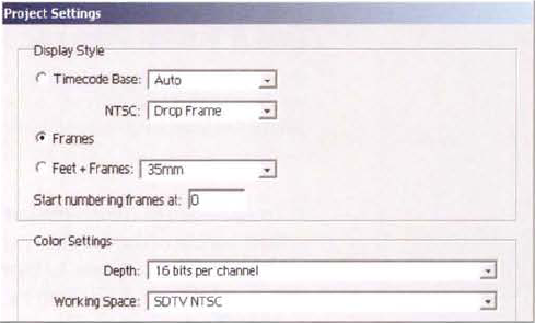
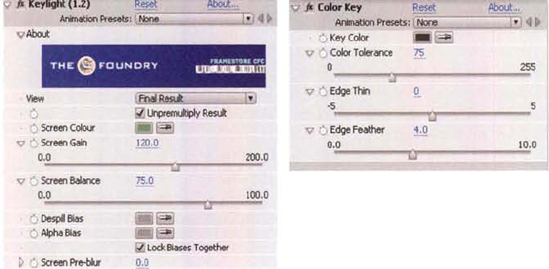
Figure 2.19. The initial composite. The brightness, contrast, and color of the statue will be adjusted in the Chapter 3 After Effects follow-up tutorial.

Nuke Tutorial 2: Working with DPX and Cineon Files

You're working on a project with specific image bit depth and image format limitations. Greenscreen footage is shot on 35mm and is provided to you as 10-bit log Cineon files. Effects footage is culled from the studio's offline shot library; 10-bit log DPX is the only format available. Background plate footage is shot with an HD digital video camera. The 12-bit linear TIFF files are converted to 16-bit before they are handed to you. Your composite is part of a visual effects job for a feature film. Therefore, you must deliver 10-bit log Cineon files to the DI house. Nevertheless, you will need to have your work approved by your supervisor. You're using an LCD monitor to judge your work. Although the monitor is calibrated, it can only approximate the log quality of film.

You can take the following steps in Nuke to set up a new composite:

1. Create a new script. Choose Edit → Project Settings. In the properties panel, set Frame Range to 1, 30, set Fps to 30, and change the Full Size Format menu to 2k_Super_35mm(Full-ap). Switch to the LUT tab. Note that the Viewer is set to sRGB, 16-Bit is set to sRGB, and Log Files is set to Cineon.

2. RMB+click over the Node Graph and choose Image → Read. Open the Read1 node's properties panel. Browse for bg_plate.tif, which is included in the Footage folder on the DVD. Note that the Colorspace menu is set to Default. Since the16-Bit menu is set to sRGB in the Project Settings properties panel, the TIFF is interpreted through the sRGB LUT. The 16-Bit preset is designed for any integer data greater than 8-bits. The plate features a city street (see Figure 2.20).

   

   Figure 2.20. (Left) Background plate (Right) Unaltered greenscreen file. Since the file is a 10-bit log Cineon, it appears washed out in the sRGB color space of the viewer.

3. RMB+click over the Node Graph and choose Image → Read. Browse for greenscreen.cin, which is included in the Footage folder on the DVD. In the Read2 node's properties panel, select the Raw Data check box. This prevents the Read node from applying a log-to-linear conversion. This causes the statue against greenscreen to appear washed out in the sRGB color space of the viewer (see Figure 2.20).

4. RMB+click over the Node Graph and choose Image → Read. Browse for the effect.##.dpx footage, which is included in the Footage folder on the DVD. Select the Raw Data checkbox. Because the footage is only 1K in resolution, it will not fit the 2K composition properly. To fix this, select the Read3 node, RMB+click, and choose Transform → Reformat. With the default settings, the Reformat1 node resizes the footage to the project output size.

5. Select the Read2 node, RMB+click, and choose Color → Log2Lin. Connect the Viewer1 node to the Log2Lin1 node. (Whenever you need to view the output of a node, reconnect the Viewer1 node or create a new viewer via Viewer → Create New Viewer.) The Log2Lin1 node, with its default settings, restores contrast to the statue (see Figure 2.21). For more information on the Log2Lin node, see "Log-to-Linear Conversions in Nuke" earlier in this chapter.

6. With the Read3 node selected, RMB+click and choose Color → Log2Lin. The default Log2Lin2 node settings are also suitable for the linear conversion of the fire footage.

   

   Figure 2.21. Detail of Cineon greenscreen footage after the application of a Log2Lin node

7. Select the Log2Lin1 node, RMB+click, and choose Keyer → Keyer. To remove the greenscreen from the statue quickly, open the Keyer1 properties panel and change Operation to Greenscreen. LMB+drag the bottom-left yellow bar in the Range field to the far right (see Figure 2.22). The green remains, although it is darkened. To remove the green completely, choose the Keyer1 node, RMB+click, and choose Merge → Premult. The Premult node multiplies the input RBG values by the input alpha values (created by the keyer). Since Nuke expects premultiplied input when merging, the output is properly prepared for the viewer. (In this case, the Keyer1 output is merged with the empty black background.) For more information on merge nodes, premultiplication, and keyers, see Chapter 3. To examine the resulting alpha channel, connect a viewer to the Premult1 node, click the Viewer pane, and press the A key. To return to an RGB view, press A again.

   

   Figure 2.22. (Left) The Keyer1 properties panel with adjusted Range field handle (Right) Detail of resulting alpha channel (black indicates transparency)

8. Select the Log2Lin2 node and apply new Keyer and Premult nodes. Leave Operation set to Luminance Key. There's no need to adjust the Range field bars since there is a high level of contrast in the image of the fire.

9. With no nodes selected, RMB+click in the Node Graph and choose Merge → Merge. Connect input A of the Merge1 node to the Premult2 node (belonging to the fire effect). Connect input B of the Merge1 node to the Read1 node (which holds the city plate). See Figure 2.23 for the completed node network. This places the fire on top of the sky. Open the Merge1 node's properties panel, and change the Operation menu to Screen. This blends the fire more naturally. (The Screen mode is detailed in Chapter 3.)

   

   Figure 2.23. The completed node network

10. With no nodes selected, RMB+click in the Node Graph and choose Merge → Merge. Connect input A of the Merge2 node to the output of the Premult1 node (belonging to the statue). Connect input B of the Merge2 node to the output of the Merge1 node. This places the statue on top of the fire/city composite. Unfortunately, the statue is floating slightly off the ground. To remedy this, select the Read2 node, RMB+click, and choose Transform → Position. A Position node is inserted between the Read2 and Log2Lin1 nodes. Open the Position node's properties panel and change Translate X and Y to −12, −45. The statue moves to a more believable location (see Figure 2.24).

11. At this stage, the statue's brightness and color does not match the background plate. In addition, the edge of the statue is "hard" compared to the surrounding scene. Both of these issues will be addressed in a Nuke follow-up tutorial in Chapter 3. In the meantime, save the file under a new name. A sample script is included as nuke2.aep in the Tutorials folder on the DVD.

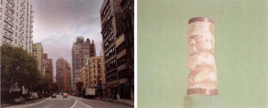
Figure 2.24. The initial composite. The brightness, color, and edge quality of the statue will be adjusted in the Chapter 3 Nuke follow-up tutorial.

Jason Greenblum started in the industry as an art department production assistant. He was serving as an art department coordinator at Digital Domain on Supernova when he made the transition to compositing. He went on to work at Rhythm & Hues and Weta Digital. In 2004, he joined Sony Pictures Imageworks. Jason's roster of feature film work includes How the Grinch Stole Christmas, Harry Potter and the Sorcerer's Stone, the second and third Lord of the Rings installments, and the second and third Spiderman sequels. He has served as a senior and lead compositor on recent projects.

Jason Greenblum at his compositing workstation. Note the dual CRT displays.

Sony Pictures Imageworks began operation in 1993. The studio creates visual effects and character animation for a wide range of feature film projects and has earned a number of Oscar nominations. Imageworks's sister company, Sony Pictures Animation, opened in 2002 to create feature animation projects such as Open Season and Surf's Up!

(Compositing falls under the lighting department at Sony Pictures Imageworks.

(Left) The front entrance to the Sony Pictures Imageworks Culver City facility (Right) One of the many art deco style buildings tucked behind rows of trees (Right photo courtesy of Sony Pictures Imageworks)

LL: What is the main compositing software used at Sony Pictures Imageworks?

JG: We have a proprietary package that we use that we've been writing (Katana). We've actually just moved over to it the last six months.... We used to use a tool called Bonzai, which was written to replace Composer. We do have a little bit of Shake. We tend to keep other tools in-house so that we can evaluate them. Everything has its own niche that it can be used for.

LL: Can you describe Katana in more detail?

JG: Because it's a 3D engine, it's got the 3D viewer—it's got all the attribute setting tools that you would need to render through Renderman—there are very clean ways to get from that to the 2D world. [For example], you can put images on planes and [create] environments, or get tracking data from a 3D scene into your comp [so that it] can be applied to roto (rotoscope).

LL: As a compositor, what involvement do you have with color management?

JG: [We had] a really cool process at Weta that made the images less breakable. The idea is to neutralize the plate when it comes to you. So it gets scanned and it goes to color timing where it's neutralized—you essentially try to make your 18 percent gray and then, since everything goes to a digital intermediate (DI) these days, [there's] a temp color timing number that they will give [the compositor] that can be looked at to see if the images are going to track. As long as you're compositing to that neutral plate and you match everything to the neutral plate, [when] they crank everything around in the DI, you're safe. [At Sony Pictures Imageworks], it's a similar process [compared to the one used at Weta]....

LL: What bit depth do you work in at Sony Pictures Imageworks?

JG: In the last two years, it's become fully float. Textures are painted in float, renders are done in float, [and] the composite is done in float. The only thing that isn't float [are the scans of the live-action plates]. They're 10-bit Cineon files.

LL: Is there any special calibration applied to the compositors' monitors?

JG: On the show I'm currently working on (G-Force), we have an environment where, while in the composite, we're looking at things in a one-stop-up, color-timed environment. Since it's a linear float, we can back out those color timing numbers into the Raw [files]. [That is], we write out a [un-color-timed] Raw with our images comped into it. We also write out a color-timed [version] that we can show the director. The DI house will get a Raw composite....

LL: Are LUTs used to create the proper viewing environment?

JG: You used to have a [software-based] monitor LUT that would take you from a log space into more of a viewable space. Now, most of that is done in the monitor for the compositing tool. What's nice about our proprietary [system] is that it has stopping-up [and] stopping-down tools within the hardware accelerator itself. So it's really easy to look into your blacks or look at it with different LUTs applied to it.

LL: Are the monitors calibrated?

JG: Our monitors are meant to be calibrated monthly if you're doing color-sensitive work. We'll have two CRTs next to each other because they're still the best calibratable viewers, and you tend to see how fast they drift because you have one next to the other—you'll see one go warm and one go cool....

Rod Basham started in the industry as a visual effects editor. While at Cinesite, he worked on such features as Air Force One and Sphere. He joined Imaginary Forces in the same capacity but was soon able to train under an Inferno artist. He shifted his concentration to Inferno compositing and has since worked on visual effects and title sequences for such films as Minority Report, Blade: Trinity, and Charlotte's Web and a host of television commercials and related projects.

Rod Basham in his Inferno bay. He uses a HD CRT among other monitors.

Imaginary Forces is a design studio with offices in Los Angeles and New York. It creates film titles, commercials, broadcast design, experience design, and general branding. The studio's recent work includes title sequences for the feature film Beverly Hills Chihuahua and the television show Mad Men.

LL: You work on an Autodesk Inferno in a 12-bit environment. Do you output 12-bit footage?

RB: Our broadcast deliverables are always 10-bit when going to DigiBeta or HDCam. Our film drops go out as [10-bit] DPXs or Cineons. So for us to go from 12-bit to 10-bit is a good thing. Most of our conversions or LUTs are set up to go from 10 to 12 or 12 to 10. [The bit depth] is high enough that we don't get any banding.

LL: When you receive live-action footage, what format is it in?

RB: We typically receive 10-bit log DPX files. Everything we generate internally is generated in linear space. Because we're so graphic heavy, it makes more sense to keep everything in a linear pipeline. So, if we receive logarithmic material, we make it linear. [A]t the end, we turn everything back into a log file.

LL: When your work is destined for film, what type of color space issues arise?

The Imaginary Forces facility in the heart of Hollywood (Image courtesy of Imaginary Forces)

RB: [D]igital intermediates are one of the biggest things to have [affected] me over the last few years. We used to have a Celco [film recorder] here, so we would actually deliver negative for our projects. A big part of my learning was figuring out how to get things from Inferno to the Celco and onto film correctly. That, happily, has gone away. Now, when you're delivering work to a DI facility, you have another level of quality control. The biggest challenge we have is that [each] DI facility may [use a different lab and a different] film stock for their film-outs. I can take one frame and make a Cineon [file] and send it to nine different [facilities] with nine different screening rooms and it will look [nine different ways]. (Other factors include the different display systems, 3D LUTs, and projector color spaces.) In fact, we've started working on a digital handshake where we call the facilities up [and have them] send us a 3D display LUT [from their DI software, whether it is True Light or Lustre]. I'll load that up into Inferno, convert my work to Cineon 10-bit log, and then view it through the 3D display LUT to see how much our work is being damaged from its original linear presentation. It's my job, from this lin[ear]-to-log conversion, to know how to [return] the colors to where they need to be when the work goes to the DI setup....

LL: For commercials, do you do the final color grading in-house?

RB: The final color grading happens here. We do it in the Flame.

LL: Do you calibrate your monitors?

RB: We have a technician who comes in periodically and does our monitors for us. Our biggest challenge these days is the different flavors of monitors. When it was all CRT, it was very straightforward. [Now], we have LCDs, CRTs, and plasma [screens]. We try to keep them all very close; they will never be exact. In fact, we just purchased one of the last remaining HD CRTs in town.