
"If you're comparing 35mm to the state-of-the art digital video, digital video cameras can at least capture 4K. If you need a hi-res scan of 35mm, the film grain gets a little big."

The digital intermediate (DI) represents one of the most significant changes to filmmaking to occur in recent years. Hence, it's important for compositors to understand the DI process, even if they are not directly involved with the editing, conforming, calibration, or color grading process. Nevertheless, color grading approaches used by DI colorists may be applied by compositors to projects that do not have the luxury of DI. Whereas DI is ultimately an optional step for a production, noise and grain are a permanent part of the production equation. That is, all film and video footage contains some form of noise or grain. Hence, the artifacts must be removed from footage or added to imported CG, digital artwork, or motion graphic elements so that the end composite is coherent and consistent. With the tutorials in this chapter, you'll have the chance to practice color grading techniques as well as disguise unwanted posterization with noise.

A digital intermediate (DI) is digital copy of a captured image. The copy is created for the purpose of digital manipulation. Once the manipulation is complete, the manipulated copy is output to the original capture format. Hence, the copy serves as an "intermediate."
In the realm of motion pictures, DI has come to indicate a common practice whereby the following workflow is used:
Motion picture footage is digitized.
The footage is edited offline (see the next section).
An edit decision list (EDL) is created for the edit. The EDL is used to conform the footage for the color grading process.
LUTs are generated and applied for proper viewing.
Titles, motion graphics, and visual effects shots may be added, but only after the editor has determined their placement and length (in which case, the EDL and conform are brought up-to-date).
The resulting footage is color graded. Color grading is carried out by specialized artists known as colorists.
The color graded result is rendered at full resolution and filmed out (captured onto film through a film recorder).
Motion picture footage is digitized with dedicated pieces of hardware. Although the hardware varies by manufacturer, it shares basic similarities:
The film is moved through the device, one frame at a time. Each frame is illuminated. The illumination is provided by a laser, LEDs, or more traditional metal halide bulbs. The light is separated into RGB components by a prism or dichroic (color-splitting) mirrors.
The RGB light is captured by charge-coupled device (CCD) chips, complementary metal oxide semiconductor (CMOS) chips, or a set of photodiodes. The RGB information is encoded into the image format of choice.
Common film formats that are scanned include 16mm, Super 16mm (single-sprocket 16mm with expanded image area), full-aperture 35mm (35mm lacking an optical soundtrack but possessing an expanded image area), and VistaVision (a 35mm variant where the image is rotated 90° for better resolution). Common scanning resolutions include standard SD, standard HD (1920Open the Read31080) and 2K full aperture (2048×1556) The digitized frames are generally stored as 10-bit log Cineon or DPX files (see Chapter 2, "Choosing a Color Space"). Other format variations, such as 16-bit linear TIFF or 16-bit log DPX, are not unusual. Some scanner manufacturers provide software that can automatically detect dust, scratches, and similar defects and remove them from the scanned image.
Conforming, as it applies to DI, is the organization and assembly of sequences and shots in preparation for color grading. The conforming process is driven by an EDL, which is updated as the editing of the footage progresses. The actual editing does not occur as part of the color grading session. Instead, editing is created offline. For offline editing, a low-resolution copy of the original footage is used. The lower resolution is necessary for speed and efficiency. Because the editing is applied to a copy, the original digitized footage remains unscathed. When the editing is complete, the EDL is exported as a specialized file that includes pertinent information for each cut shot (film reel, starting frame number, and so on).
Conforming may be carried out by specialized software, such as Autodesk Backdraft Conform. This assumes that the conformed footage is accessible by compatible color-grading software, such as Autodesk Lustre. It's also possible to conform and color grade with a single piece of software. For example, Assimilate Scratch and Da Vinci Resolve are designed to carry out both tasks. (While some DI systems are purely software based, others require matching hardware.)
An equally important step in the DI process is the application of LUTs. As discussed in Chapter 2, color calibration is an important consideration to a compositor. A compositor should feel confident that their work will look the same on a workstation as it does in the final output, whether it is film or video. In addition to the careful selection of working color spaces, it's important to apply monitor calibration. When a monitor is calibrated, a LUT is stored by a color profile. The LUTs discussed thus far are one-dimensional arrays of values designed to remap one set of values to a second set. If a LUT is designed to remap a single color channel, it is considered a 1D LUT. If a LUT is designed to remap three channels, such as RGB, then a 1D LUT is applied three times. Because monitor and projector calibration is critical for DI and color grading, however, 1D LUTs become insufficient. Thus, 3D LUTs are employed.
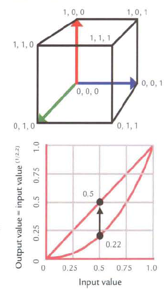
A 3D LUT is a three-dimensional look-up table that defines input and output colors as triplets (three values corresponding to three channels, such as RGB). 3D LUTs can be represented by an XYZ color cube (see the top of Figure 8.1). Two of the corners of the cube correspond to black and white. Three of the corners correspond to primary red, green, and blue. Three of the corners correspond to secondary colors yellow, cyan, and magenta. Any given color has an X, Y, Z location within the cube. When two different color spaces are compared, they do not share the same space within the visible spectrum. Hence, the deformation supplied by a 3D LUT fits one color space within a second color space. As such, the alteration of a single color channel affects the remaining color channels. The influence of one color component on the remaining components is known as color cross-talk. Color cross-talk is a natural artifact of motion picture film, which relies on cyan, magenta, and yellow dyes; when film stock is developed, it's impossible to affect a single dye without affecting the other two. In comparison, a 1D LUT can only affect one channel at time (see the bottom of Figure 8.1). For example, remapping the red channel does not affect the green and blue channels. For efficiency, the 3D LUT deformation is carried out by a deformation lattice. The lattice has a specific resolution, such as 17×17×17. Color points that do not fall on a lattice point must be interpolated. Software that employs 3D LUTs may apply its own unique interpolation method.
Based on their architecture, 3D LUTs offer the following advantages over 1D LUTs:
The saturation of an input can be altered.
Cross-talk is intrinsically present. Thus, the color space of motion picture film can be more accurately represented.
Color space conversions between devices with different gamuts are easily supported.
Soft clipping is feasible. Whereas a standard clip leaves a hard transition between non-clipped and clipped values, soft clipping inserts a more gradual transition. Soft clipping is useful when converting to or from a low-bit-depth color space.
Posterization is less likely to occur with the color space conversion.
At the same time, 1D LUTs retain some advantages:
They're easy to generate with a wide range of calibration software.
Interpolation of color points is not required, so accuracy may be greater in some situations.
1D LUTs and 3D LUTs are both stored as text files that feature columns of numeric values. 1D and 3D LUTs can be carried by ICC profiles. Due to their complexity, 3D LUTs are usually generated by specialized software. For example, Arricube Creator, part of Arri's family of DI tools, is able to create 3D LUTs and package them as color profiles for a wide range of devices. In addition, Nuke can generate 3D LUTs internally, as is discussed in the section "3D LUTs in Nuke" later in this chapter.
If a project is slated for DI, a decision must be made whether or not an effects shot (using titles, motion graphics, or visual effects) should be pre-graded (color graded in advance). For example, if an animation/compositing team is given a live-action plate to which effects must be added, three approaches are possible:
The animation/compositing team matches the effects work to the ungraded plate.
The plate is pre-graded at the visual effects studio and is handed off to the animation/compositing team.
The sequence that will host the effects shot is color-graded by a colorist at an outside color grading facility. The plate to be used for the effects shot is color-graded to match the sequence and then is delivered to the visual effects studio.
With pre-grading, the plate may be neutralized, whereby the median pixel value is established as 0.5, 0.5, 0.5. Neutralization prevents bias toward red, green, or blue, which creates a color cast. In addition, neutralization allows the colorist to provide the animation/compositing team with color grading values so that they can roughly preview the final color look on their own workstations. Alternately, the colorist may apply a quick color grade to the plate to match the final look of the surrounding scene. Pre-grading is particularly useful on effects-heavy feature film work, where hundreds of effects shots would otherwise slow the final color grading process. However, pre-grading may lead to an accentuation of undesirable artifacts as the plate is repeatedly color graded. In comparison, if the effects work is matched to the ungraded plate, the color may be significantly different from what the director, art director, or visual effects supervisor may have imagined. In such a case, the effects approval process may prove difficult. In addition, matching CG to an ungraded plate may be more challenging if the footage is underexposed, has a heavy color cast, or is otherwise washed out.
Once an effects shot is completed, it is imported into the DI system and conformed to the EDL (the editor receives a copy so that it can be included in the offline edit). A final color grading is applied to match the surrounding scene. If the effects shot utilized a pre-graded plate, the final grading is less intensive.
Color grading generally occurs in several steps, brief descriptions of which follow:
Primary Grading Each shot is graded to remove strong color cast or to adjust the exposure to match surrounding shots. The grading is applied to the entire frame.
Secondary Grading Grading is applied to specific areas of a shot. For example, the contrast within unimportant areas of the composition may be reduced, thus shifting the focus to the main characters. Specific pools of light may be given a different color cast for aesthetic balance. Areas with an unintended mistake, such as an unwanted shadow, may be darkened so that the mistake is less noticeable.
Specific areas within a shot are isolated by creating a mask, through the process of keying, or via the importation of a matte rendered in another program, such as After Effects. Masking may take the form of primitive mask shapes or spline-based masking tools. Keyers are able to key out specific colors or luminance levels and thus produce hicon (high-contrast) or luma mattes. Built-in rotoscoping and tracking tools are also available (although they are generally less refined to those found in compositing packages). Masked areas within a frame on a color grading system are commonly known as power windows.
The actual grading is carried out by a set of standard tools, which provide a means to adjust brightness, contrast, gamma, gain, pedestal (lift), hue, saturation, and exposure per channel. Each of these functions in a manner similar to the various sliders supplied by the effects and nodes found in After Effects and Nuke. (For more information on color manipulation, see Chapter 4, "Channel Manipulation.") In addition, tools are used to affect the color balance and tint. Color balance adjusts the strength and proportion of individual color channels. Tint increases or decreases the strength of a particular color.
If a project is destined for multiple media outlets, multiple color grading sessions may be applied. For example, separate color grades may be created for a traditional theatrical release and an HDTV broadcast.
Ultimately, the goal of color grading can be summarized as follows:
To make the color balance of all shots within a scene or sequence consistent and cohesive
To correct or accentuate colors recorded by cinematographers, who may have a limited amount of time on set to fulfill their vision
To produce color schemes that match the intention of the director, production designer, and art director
To have the color-graded result appear consistent in a variety of outlets, including movie theater screens and home living rooms
DI is not limited to motion picture film. Digital video or computer animation footage is equally suitable for the DI process and can benefit from DI color grading tools. The main advantage of video and animation in this situation is that scanning is not necessary. Thus, the basic workflow follows:
The footage is conformed to an EDL.
LUTs are generated and applied for proper viewing.
In the case of video, titles, motion graphics, and/or visual effects shots are integrated. In the case of animation, titles and/or motion graphics are integrated. In both situations, the editor determines the placement and duration and updates the EDL.
The resulting footage is color graded.
The color-graded result is recorded to video or film.
Although tape-based video must be captured, tapeless systems that utilize hard disks or flash memory are becoming common. In fact, various DI software systems, including Autodesk Lustre and Digital Vision, have recently added direct support for propriety Raw formats generated by digital video camera systems such as RED One and Arri.
Television commercials, music videos, and other short-form video projects have enjoyed the benefits of the DI process for over two decades. For example, Autodesk Flame (developed by Discreet Logic) has been in use since the mid-1990s and has provided efficient digital footage manipulation throughout its history. Going back further in time, the Quantel Harry allowed the manipulation of stored digital video as early as 1985.
Telecine machines, which are able to convert motion picture film to video in real time, have been in use since the early 1950s. Real-time color-grading capacity was added to the telecine process in the early 1980s. In contrast, high-quality motion picture film scanners were not available until Kodak introduced the Cineon DI system in 1993. Film scanners share much of their technology, including dichroic mirrors and color-sensitive CCDs, with telecine machines. In fact, there is such a high degree of overlap between the two systems that the word telecine is used as a generic term for all film transfers.
Fully animated CG features have also tapped into the power of the DI process. For example, with The Incredibles (2004) and Surf's Up (2007), no shot was filmed out until the entire project was sent through the DI process. DI offers the ability to fine-tune colors across sequences in a short amount of time. Without DI, matching the color quality of every shot in a sequence tends to be time-consuming because multiple artists may work on individual shots for weeks or months.
As a compositor, you may not be directly involved with the DI process. In fact, you may work on a project that does not employ DI or color-grading sessions by a dedicated colorist. As such, you may find it necessary to apply your own color adjustments. In this situation, the techniques developed by colorists are equally applicable.
As discussed in the section "DI Color Grading" earlier in this chapter, color grading generally occurs in two steps: primary and secondary. Primary grading applies adjustments to the entire frame of a shot. Secondary grading applies adjustments to limited areas within the frame. To isolate areas with After Effects, you can use the Pen tool to draw masks or create hicon or luma mattes through the combination of various effects. For more information on masking, see Chapter 7, "Masking, Rotoscoping, and Motion Tracking." For an example of luma matte creation, see Chapter 3, "Interpreting Alpha and Creating Mattes."
For grading adjustments, standard color correction effects supply sliders for the most common grading tasks. A list of tasks and corresponding effects follows:
Brightness: Brightness & Contrast, Curves, Levels
Gamma: Gamma/Pedestal/Gain, Levels, Exposure
Contrast: Brightness & Contrast, Curves, Levels
Gain: Gamma/Pedestal/Gain
Pedestal: Gamma/Pedestal/Gain, Exposure (Offset property)
Hue: Hue/Saturation
Saturation: Hue/Saturation
Exposure: Exposure
Color Balance: Color Balance, Curves, Levels (Individual Controls)
Tint: Hue/Saturation, Tint
For details on each of the listed effects, see Chapter 4, "Channel Manipulation." The section "AE Tutorial 8: Color Grading Poorly Exposed Footage" at the end of this chapter steps through the grading process.
As discussed in the section "DI Color Grading" earlier in this chapter, color grading generally occurs in two steps: primary and secondary. Primary grading applies adjustments to the entire frame of a shot. Secondary grading applies adjustments to limited areas within the frame. To isolate areas with Nuke, you can use the Bezier node to draw masks or create hicon or luma mattes through the combination of various nodes. For more information on masking, see Chapter 7, "Masking, Rotoscoping, and Motion Tracking." For an example of luma matte creation, see Chapter 4, "Channel Manipulation." As for grading adjustments, standard Color nodes supply sliders for the most common grading tasks. A list of tasks and corresponding effects follows:
Brightness: HSVTool, HueShift, Grade
Gamma: ColorCorrect, Grade
Contrast: ColorCorrect
Gain: ColorCorrect, Grade
Lift (Pedestal): ColorCorrect, Grade
Hue: HSVTool, HueCorrect, HueShift
Saturation: HSVTool, HueCorrect, ColorCorrect, Saturation
Color Balance: HueCorrect
Although the word Brightness can only be found in the HSVTool's or HueShift's properties panel, the adjustment of Gain, Offset, or Whitepoint sliders of other nodes will have a similar effect. As for color balance, you are not limited to the HueCorrect node. Any node can affect a single channel and thereby change the balance of all three color channels. For example, if you deselect the Red and Green check boxes of a Grade node, the Grade node affects only the Blue channel. If the Grade node is then adjusted, the overall color balance changes.
As for tinting an image, there is no direct correlation to the After Effects Tint effect or Colorize option of the Hue/Saturation effect. However, to create a similar look, you can merge the output of a Constant node (Image → Constant) with a Read node. If the Merge node's Operation menu is set to Multiply, the tinting is thorough (see Figure 8.2).

Figure 8.2. (Top) Input image (Center) Node network with a red-colored Constant node (Bottom) Tinted result. A sample Nuke script is included as tint.nk in the Tutorials folder on the DVD.
It's also possible to tint an image by assigning the Whitepoint or Blackpoint parameters a non-monochromatic value. For a demonstration of this technique, see the section "Nuke Tutorial 8: Color Grading Poorly Exposed Footage" at the end of this chapter. For details on each of the nodes listed in this section, see Chapter 4, "Channel Manipulation."
As discussed in Chapter 2, Nuke provides a set of 1D LUTs (which may be viewed through the Project Settings properties panel). The LUTs are designed to convert the color space of a file to Nuke's internal color space. The goal is to display the file image correctly on the system monitor via Nuke's viewer. In addition to 1D LUTs, Nuke supports the importation and creation of 3D LUTs. You can find the nodes in the Color and Color → 3D LUT menus.
The TrueLight node loads 3D LUTs created by FilmLight TrueLight. TrueLight is a color management system comprising hardware and software modules. The TrueLight node is designed to display film-based images on a linear RGB monitor properly.
The Vectorfield node loads a custom 3D LUT. The 3D LUT can take the form of a TrueLight LUT (.cub or .cube), Assimilate Scratch and Autodesk Lustre LUTs (.3dl), or native Nuke vector field (.vf) text file.
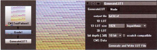
When CMSTestPattern and GenerateLUT are used together, they create a custom 3D LUT. CMSTestPattern is a special test pattern that features colored stripes of known values. The output of the CMSTestPattern node must be connected to some type of color correction node (or nodes). In turn, the output of the color correction node is connected to a GenerateLUT node (see Figure 8.3) Whatever adjustments are made to the color correction node are stored as a 3D LUT when the Generate And Write LUT File button is pressed in the GenerateLUT node's properties panel. You can chose to save the 3D LUT as a TrueLight LUT (.cub or .cube), Assimilate Scratch or Autodesk Lustre LUTs (.3dl), native Nuke vector field (.vf), or color management system format (.cms). The 3D LUT may then be used by another program or by Nuke's Vectorfield node. The size of the 3D LUT is set by the CMSTestPattern node's RGB 3D LUT Cube Size cell. Although the cell defaults to 32, a common size used for 3D LUTs is 17. (17 implies that the color cube is 17×17×17.)
If you rename a Vectorfield node VIEWER_INPUT, the listed 3D LUT will be applied to the viewer when the Input Process (IP) button is toggled on. The IP button rests to the right of the Display_LUT menu at the top right of the Viewer pane (see Figure 8.4).

By creating a custom 3D LUT, loading it into a Vectorfield node, and activating it with the IP button, you can quickly view log images as if they have been converted to a linear color space. To do so, follow these steps:
Choose Color → 3D LUT → CMSTestPattern and Color → Colorspace. Connect the output of the CMSTestPattern node to the input of the Colorspace node (see Figure 8.5). In the Colorspace node's properties panel, set the In menu to Cineon. Set the Out menu to sRGB.
Choose Color → 3D LUT → GenerateLUT. Connect the output of the Colorspace node to a GenerateLUT node. In the GenerateLUT node's properties panel, enter an output file name and click the Generate And Write LUT File button.
Choose Color → 3D LUT → Vectorfield. Rename the Vectorfield node VIEWER_INPUT. In the Vectorfield's node's properties panel, load the recently written 3D LUT file. A sample LUT file is included as
3dlut.vfin the Footage folder on the DVD.Using a Read node, import a Cineon or DPX file. Open the Read node's properties panel. Select the Raw Data check box. This prevents the Read node from applying a log-to-linear conversion. Change the Display_LUT menu (in the Viewer pane) to Linear. The file appears washed out in the viewer. Toggle on the IP button (so that the letters turn red). The viewer temporarily shows a log-to-linear color space conversion without affecting the imported log file or altering the node network.

Note that the Display_LUT menu applies a 1D LUT after the application of the 3D LUT that is activated by the IP button. To see an accurate color space conversion, set Display_LUT to Linear, which essentially disables the 1D LUT application. (For more information about project 1D LUTs, see Chapter 2, "Choosing a Color Space.")
Noise, in the realm of image processing, is a random fluctuation in image brightness. With a CCD or CMOS chip, noise takes the form of shot noise, which is visible as 1-pixel deviations in the image (see Figure 8.6). Shot noise is a result of statistical variations in the measurement of photons striking the sensor. In common terms, this arises from an irregular number of photons striking the sensor at any given moment. Shot noise is most visible when the exposure index (ISO speed) is high, which is often necessary when you're shooting in a low-light situation. This is due to a relatively small number of photons striking the sensor. With few photons, variations in the photon count are more noticeable. Hence, you may not see shot noise when you're photographing a brightly lit subject. Shot noise can also occur within an electronic circuit where there are statistical variations in the measurement of electron energy.
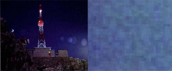
Figure 8.6. (Left) Night shot with low light level (Right) Detail of shot noise visible in the lower-right sky (Photo © 2009 by Jupiterimages)
When 1-pixel noise is intentionally applied to an image, it's known as dither and the application is referred to as dithering. Dithering is often necessary to disguise quantization errors, which are unwanted patterns created by the inaccurate conversion of analog signals to digital signals. For example, the conversion of analog video to digital images may create posterization due to mathematical rounding errors. Dithering is also useful for improving the quality of low-bit-depth display systems, although improvements in hardware have made this no longer necessary.
A third type of noise occurs as a result of image compression. For example, digital video must be compressed. Most compression schemes are lossy; that is, the compression operates on the assumption that data can be lost without sacrificing basic perceptual quality. Compression allows for significantly smaller files sizes. However, the compression leads to artifacts such as posterization and irregular pixelization. Although the artifacts may be very subtle, adjustments to the image contrast or gamma soon make them visible (see Figure 8.7). Similar pixelization may also result from the improper de-interlacing of video footage, where blockiness appears along high-contrast edges.

Figure 8.7. (Left) Detail of video greenscreen footage. White box indicates area of interest. (Center) Enlargement of greenscreen with an increase in contrast (Right) Same enlargement in grayscale
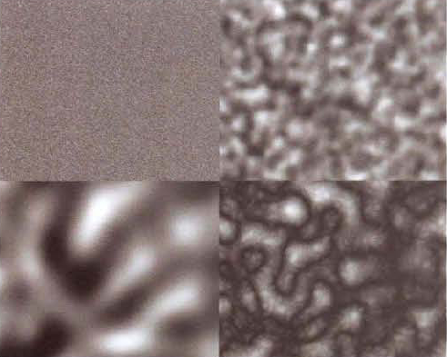
Grain, on the other hand, is a form of noise inherent in motion picture film and film-based photography. The grain occurs as a result of the irregular silver-halide crystals embedded in the film emulsion (see Figure 8.8).

Figure 8.8. (Left) Enlargement of 35mm film grain (Right) Same grain desaturated. Note the similarity to Perlin noise in Figure 8.9
In contrast, CG and similar digital graphics do not carry electronic noise or grain (unless there is improper anti-aliasing). As such, it becomes necessary to add noise to the graphics or remove noise from live-action footage. If this step is not taken, the integration of the graphics with the live action will not be as successful. At the same time, noise and grain are useful when you want to make one format emulate another. For example, if you apply grain to video, you can emulate motion picture footage.
3D, digital imaging and compositing programs can generate noise. This is often a handy way to create an organic, seemingly random pattern. Once the noise is generated, it can be used as matte or other input to help create a specific compositing effect.
When a compositor generates noise, it is usually based upon a Perlin noise function. Perlin noise was developed in the mid-1980s by Ken Perlin as a way to generate random patterns from random numbers. Perlin noise offers the advantage of scalability; the noise can be course, highly detailed, or contain multiple layers of coarseness and detail mixed together (see Figure 8.9).
Perlin noise is a form of fractal noise. A fractal is a geometric shape that exhibits self-similarity, where each part of the shape is a reduced-sized copy of the entire shape. Fractal patterns occur naturally and can be seen within fern fronds, snowflakes, mountain ranges, and various other plant, crystal, and geographic occurrences.
After Effects and Nuke provide several effects and nodes with which to create or remove noise and grain.
After Effects noise and grain effects are found under the Noise & Grain menu. Five of the most useful ones are detailed in the following three sections.
The Fractal Noise effect creates a Perlin-style noise pattern. You can choose one of 17 variations of the noise by changing the Fractal Type menu. By default, the layer to which the effect is applied is completely obscured. However, you can override this by switching the Blending Mode menu to one of the many After Effects blending techniques. By default, Fractal Noise is not animated, but you can keyframe any of its properties. For example, the Evolution control sets the point in space from which a noise "slice" is taken. If Evolution changes over time, it appears as if the camera moves through a solid noise pattern along the z-axis. The Complexity slider, on the other hand, determines the detail within the pattern. Low values create a simple, blurry noise pattern. High values add different frequencies of noise together, producing complex results.

Figure 8.10. (Top Left) Background plate (Top Right) Animated pattern generated with Fractal Noise (Bottom Left) Two iterations of the pattern positioned in 3D space and masked (Bottom Right) Iterations combined with the plate with the Screen blending mode. A sample project is saved as fractal_spec.ae in the Tutorials folder on the DVD.
The Fractal Noise effect provides a means to generate a soft, irregular, organic pattern. For example, you can adjust the Fractal Noise effect so that it mimics the specular caustic effect created when bright light hits the top of a body of water (see Figure 8.10). The result is then positioned, masked, and blended with a background plate.
In contrast, the Noise effect creates randomly colored, 1-pixel noise and adds the noise to the original layer (see Figure 8.11). By default, the Clip Result Values check box guarantees that no pixel value exceeds a normalized 0 to 1.0 range. The noise pattern automatically shifts for each frame; the animation is similar to television static.

Figure 8.11. (Left) Noise effect with Amount Of Noise set to 20% (Right) Add Grain effect with Intensity set to 3. A lower setting will make the noise much more subtle.
The Add Grain effect differentiates itself from the Noise effect by creating an irregular noise pattern (see Figure 8.11). That is, the noise is not fixed to a 1-pixel size. Additionally, the effect provides property sliders to control the intensity, size, softness, and various color traits, such as saturation. The grain pattern automatically shifts for each frame, but the rate of change can be adjusted through the Animation Speed slider. A value of 0 removes the animation. Due to its irregularity, Add Grain is superior to Noise when replicating the grain pattern found in motion picture footage and the compression artifacts found within digital video. You can emulate specific motion picture films stocks, in fact, by changing the Preset menu, which lists 13 stock types. However, when replicating the shot noise found in digital video, Noise proves superior. For more information on compression grain and shot noise, see the section "Noise and Grain" earlier in this chapter.
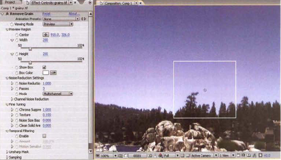
Although its task is fairly mundane, the Remove Grain filter employs sophisticated signal processing techniques. Since its operation is unusual, you can use the following steps as a guide:
Apply the Remove Grain effect to a layer containing grain. The effect will remove a portion of the grain immediately. Note that the result appears only in the white preview window in the viewer. You can interactively LMB+drag the preview window box to a new position within the viewer. To see the result of the effect over the entire layer, change the Viewing Mode menu to Final Output. To change the size of the preview window, adjust the Width and Height slider in the Preview Region section.
To reduce the aggressiveness of the removal process and any excessive blurring, lower the Noise Reduction value (in the Noise Reduction Settings section). To increase the accuracy of the suppression, raise the value of the Passes slider. If there is no change in the resulting image, return the Passes slider to a low value. High values are better suited for large, irregular grain.
To refine the result further, adjust the sliders within the Fine Tuning section. For example, if the grain is heavily saturated, raise the Chroma Suppression slider. The Texture slider, on the other hand, allows low-contrast noise to survive. To reintroduce a subtle noise to an otherwise noise-free image, increase the Texture value. Noise Size Bias targets grains based on their size. Negative values aggressively remove fine grains, while positive values aggressively remove large grains. The Clean Solid Areas slider serves as a contrast threshold; the higher the Clean Solid Areas value, the greater the number of median-value pixels averaged together (high-contrast edges are not affected).
To help identify the best property settings, you can change Viewing Mode to Noise Samples. A number of small windows are drawn in the viewer and indicate the sample areas. The program chooses sample areas that contain a minimal amount of value variation between the pixels. Such areas are used as a base reading for the noise-suppression function. In addition, you can change Viewing Mode to Blending Matte. The viewer displays a matte generated by the edge detection of high-contrast areas. The matte is used to blend the unaffected layer with the degrained version. The blending occurs, however, only if the Amount slider (in the Blend With Original section) is above 0.
If the grain is present across multiple frames, select the Enable check box in the Temporal Filtering section. Test the effect by playing back the timeline. If unwanted streaking occurs for moving objects, reduce the Motion Sensitivity value.
If the grain removal is too aggressive, high-contrast edges may become excessively soft. To remedy this, raise the Amount slider, in the Unsharp Mask section, above 0. This adds greater contrast to edges, creating a sharpening effect.
The Match Grain effect is able to identify the grain within a source layer and apply it to a target layer that carries the effect. You can use the following steps to apply Match Grain:
Create a new composition. LMB+drag the source footage (the footage that contains the grain) into the layer outline of the Timeline panel. LMB+drag the target footage (the footage that will receive the grain) into the layer outline so that it sits on top.
Select the target footage layer and choose Effect → Noise & Grain → Match Grain. A white selection box appears in the viewer (see Figure 8.13). The box indicates the area from which the grain is sampled. The sample is used to construct a new grain pattern that is applied to the entire target image. In the Effect Controls panel, change the Noise Source Layer menu to the source footage layer name. Grain appears within the selection box.
To sample the grain from a different area of the source image, LMB+drag the center handle of the selection box to a different portion of the frame. To see the result on the entire frame, change the Viewing Mode menu to Final Output.
To adjust the size, intensity, softness, and other basic traits of the grain, change the properties within the Tweaking and Color sections. To change the style of blending, adjust the properties within the Application section. If the source layer is in motion and the grain pattern changes over time, the target layer will gain animated grain.
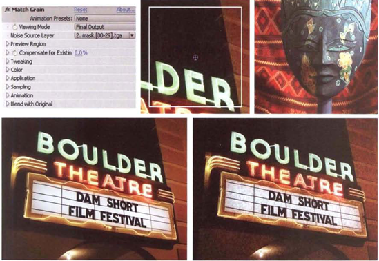
Figure 8.13. (Top Left) Match Grain properties (Top Center) The selection box, as seen in the viewer (Top Right) Source layer. Note that the video shot noise and compression artifacts, which will serve as a grain source, are not immediately visible. (Bottom Left) Grain-free target layer (Bottom Right) Result of Match Grain effect. A sample project is included as match_grain.ae in the Footage folder on the DVD.
Nuke includes several nodes that are able to replicate fractal nose, shot noise, and film grain. In addition, the program offers two nodes with which to remove film grain. The nodes are found in the Draw and Filter menus.
The Noise node creates two styles of Perlin noise: Fractional Brownian Motion (FBM) and Turbulence. You can switch between the two styles by changing the Type menu. FBM noise takes advantage of mathematical models used to describe Brownian Motion, which is the seemingly random motion of particles within a fluid dynamic system. By default, FBM noise is soft and cloudlike. In contrast, Turbulence noise produces hard-edged, spherical blobs. Regardless, both noise styles rely on the same set of parameters. The X/Y Size slider sets the frequency, or scale, of the noise pattern. Larger values "zoom" into the noise pattern detail. The Z slider allows you to choose different "slices" of the pattern. That is, if you slowly change the Z value, the virtual camera will move through the pattern as if it was traveling along the z-axis. If you want the noise to change its pattern over time, you must animate the Z parameter. The Octaves cell sets the number of Perlin noise function iterations. In essence, Octaves controls the number of noise patterns that are at different scales and are layered together. For example, if Octaves is set to 2, two noise patterns, each at a different scale, are combined through the equivalent of a Max merge. The Lunacarity slider determines the difference in scale for each noise pattern layered together. (Lunacarity, as a term, refers to the size and distribution of holes or gaps within a fractal.) The higher the Lunacarity value, the greater the difference in scale between each layered pattern. Hence, larger Lunacarity values produce a greater degree of fine detail.
Perlin-style noise is useful for creating soft, organic, animated mattes. For example, in Figure 8.14, the fluctuating illumination on a wall is created by combining a properly exposed and an underexposed version of the same wall plate. The combination of the two versions is controlled by a Noise node, which is connected to the Mask input of a Merge node. Since the Noise creates a soft, blobby pattern in grayscale, the end effect is similar to the flickering light of a flame.
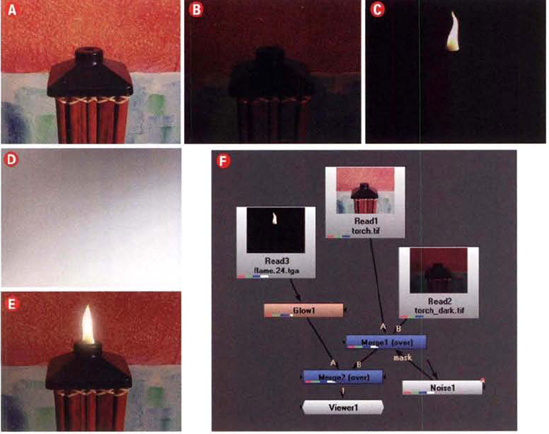
Figure 8.14. (A) Properly-exposed plate of a torch and wall (B) Underexposed version of plate (C) Flame element (D) Soft fractal pattern created by Noise node (E) Final composite (F) Node network. To see the flickering effect of the Noise node, open and play back the noise_flicker.nk script from the Tutorials folder on the DVD.
The Dither node creates a 1-pixel random pattern and is suitable for emulating shot noise. To function, it requires an input connection. The Amount slider controls the degree to which the noise pattern is mixed with the input. By default, the noise is colored. You can create a monochromatic variation by selecting the Monodither check box. The noise pattern automatically changes over time and is similar to TV static.
The Grain node reproduces grain found in specific film stocks. You can select a stock by changing the Presets menu to one of six Kodak types (see Figure 8.15). You can create a custom grain by changing any of the parameter sliders. You can set the grain size and irregularity for red, green, and blue grains. To reduce the grain's strength, lower the Red, Green, and Blue Intensity sliders. To increase the contrast within the grain pattern, increase the Black slider value. Note that the Grain node is designed for 2K motion picture scans; thus, default settings may create overly large grain sizes on smaller resolution inputs.
The ScannedGrain node (in the Draw menu) allows you to replicate the noise found within an actual piece of footage. To prepare a suitable piece of footage, follow these steps:
Shoot a gray card (see Figure 8.16). Scan or transfer the footage. Only 2 or 3 seconds are necessary.
Import the footage into Nuke through a Read node. Connect the output of the Read node to a Blur node. Raise the Blur node's Size parameter value until the noise is no longer visible. Create a Merge node. Connect the output of the Read node to input A of the Merge node. Connect the output of the Blur node to input B of the Merge node. Set the Merge node's Operation parameter to Minus. This network subtracts the gray of the gray card, leaving only the grain over black (see Figure 8.16).
Connect the output of the Merge node to the input of an Add node (Color → Math → Add). Change the Add node's Value cell to 0.5. When you add 0.5, the grain becomes brighter and the black gaps turn gray. This offset is required by the ScannedGrain node.
Write the result to disk with a Write node.

To apply the ScannedGrain node, follow these steps:
Import grain-free footage through a Read node. Connect the output of the Read node to the input of a ScannedGrain node. Connect the viewer to the output of the ScannedGrain node.
Open the ScannedGrain node's properties panel. Browse for the grain footage through the Grain cell (see Figure 8.17). The grain is added to the grain-free footage. Initially, the grain is very subtle. To increase its intensity, you can adjust the Amount parameter. The Amount parameter is split into red, green, and blue channels. In addition, you can interactively adjust the intensity of each Amount channel through the built-in curve editor. If the output becomes too bright, adjust the Offset slider.

Figure 8.17. (Left) ScannedGrain node's properties panel (Top Right) Detail of grain-free footage (Bottom Right) Same footage after the application of the ScannedGrain node. (The contrast has been exaggerated for print.) A sample script is included as scannedgrain.nk in the Footage folder on the DVD.
In Nuke, there are two specialized nodes that can remove grain: DegrainSimple and DegrainBlue. Both are found under the Filter menu.
The DegrainSimple node is suitable for removing or reducing light grain (see Figure 8.18). The aggressiveness of the grain removal is controlled by Red Blur, Green Blur, and Blue Blur sliders.
The DegrainBlue node targets noise within the blue channel without affecting the red or green channel. In general, the blue channel of scanned motion picture film and digital video is the grainiest. A single slider, Size, controls the aggressiveness of the removal.

Figure 8.18. (Left) Detail of a grainy image (Right) Result after the application of a DegrainSimple node. Note the preservation of high-contrast edges. A sample script is included as degriansimple.nk in the Footage folder on the DVD.
Keep in mind that aggressive grain removal may destroy desirable detail within the frame. While the removal is most successful on areas with consistent color, like skies or painted walls, it is the most damaging in areas when there are numerous objects or intricate textures. Therefore, it often pays to control the effect of degraining by limiting it to a masked area. In addition, Nuke's degraining nodes are unable to address irregular artifacts created by compression.
With these tutorials, you'll have the opportunity to color grade an otherwise unusable plate. In addition, you'll disguise posterization with blur and noise.
Although footage delivered to a compositor usually carries proper exposure, occasions may arise when the footage is poorly shot, is faded, or is otherwise damaged. Hence, it's useful to know how to color grade in less than ideal situations.
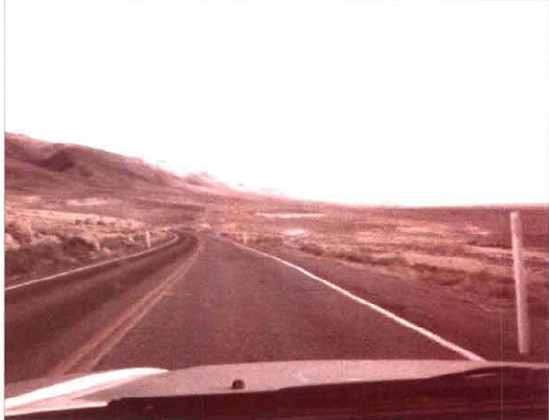
Create a new project. Choose Composition → New Composition. In the Composition Settings dialog box, change the Preset menu to NTSC D1 Square Pixel, Duration to 30, and Frame Rate to 30. Import the
road.##.tgafootage from the Footage folder on the DVD. LMB+drag theroad.##.tgafootage from the Project panel into the layer outline of the Timeline panel. Scrub the timeline. The footage features a highway as shot through the windshield of a car (see Figure 8.19). The footage is extremely washed out. In addition, the colors have shifted toward red (not unusual for old motion picture film). Choose File → Project Settings. In the Project Settings dialog box, set Depth to 16 Bits Per Channel. A 16-bit space will allow for color manipulation and is necessary for such poorly balanced footage. (Generally, you should pick a specific color space through the Working Space menu to match your intended output; however, for this exercise, Working Space may be set to None.)With the
road.##.tgalayer selected, choose Effect → Color Correction → Brightness & Contrast. Set Brightness to 25 and Contrast to 80. This restores contrast to the footage (see Figure 8.20). However, the sky becomes overexposed when the road and countryside is properly adjusted. In addition, the heavy red cast becomes more apparent.LMB+drag a new copy of the
road.##.tgafootage from the Project panel to the layer outline so that it sits on top. With the new layer selected, use the Pen tool to separate the sky (see Figure 8.21). Expand the new layer's Mask 1 section in the layer outline and set Mask Feather to 100, 100. With the new layer selected, choose Effect → Color Correction → Brightness & Contrast. Set Brightness to 10 and Contrast to 40. By separating the sky, you are able to color grade it without unduly affecting the road or countryside. Since the camera is moving, animate the mask to match the horizon line throughout the duration. (For more information on the Pen tool and masking, see Chapter 7, "Masking, Rotoscoping, and Motion Tracking.")At this point, the footage remains extremely red. To adjust the color balance of both layers, however, you will need to nest the composites. Choose Composition → New Composition. Set Comp 2 to match Comp 1. Open the Comp 2 tab in the Timeline panel. From the Project panel, LMB+drag Comp 1 into the layer outline of the Comp 2 tab. With the new Comp 1 layer selected in Comp 2, choose Effect → Color Correction → Color Balance. Adjust the Color Balance effect's sliders to remove the red and bring the colors back to a normal range. For example, the following settings produce the result illustrated by Figure 8.22:
Shadow Red Balance: −20
Shadow Green Balance: 10
Midtone Red Balance: −30
Midtone Green Balance: −10
Hilight Red Balance: −10
Hilight Green Balance: 15
Hilight Blue Balance: 20
At this stage, the footage appears fairly desaturated. To add saturation, choose Effect → Color Correction → Hue/Saturation and set the Master Saturation slider to 20. The tutorial is complete. A sample After Effects project is included as
ae8.aepin the Tutorials folder on the DVD.


Although footage delivered to a compositor usually carries proper exposure, occasions may arise when the footage is poorly shot, is faded, or is otherwise damaged. Hence, it's useful to know how to color grade in less than ideal situations.
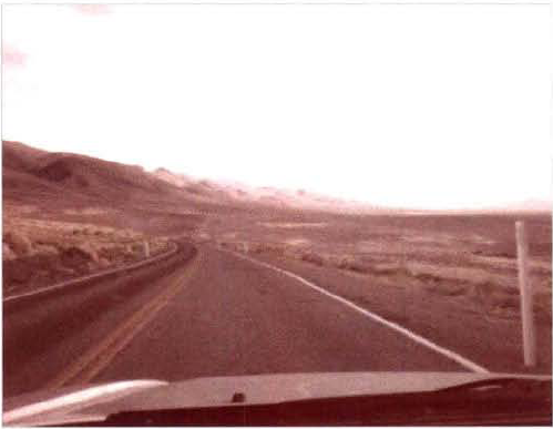
Create a new script. Choose Edit → Project Settings. In the properties panel, set Frame Range to 1, 30 and Fps to 30. Change the Full Size Format menu to New. In the New Format dialog box, set File Size W to 720 and File Size H to 540. Enter D1 as the Name and click OK. In the Node Graph, RMB+click and choose Image → Read. Through the Read1 node's properties panel, browse for the
road.##.tgafootage from the Footage folder on the DVD. Connect a viewer to the Read1 node. Scrub the timeline. The footage features a highway as shot through the windshield of a car (see Figure 8.23). The footage is extremely washed out. In addition, the colors have shifted toward red (not unusual for old motion picture film).Since the footage has no alpha channel, select the Read1 node, RMB+click, and choose Channel → Shuffle. In the Shuffle1 node's properties panel, select the white 1 check box that corresponds with the alpha channel (see Figure 8.24). An alpha channel will be necessary for proper masking.
With the Shuffle1 node selected, RMB+click and choose Color → Grade. Connect a viewer to the Grade1 node. In the Grade1 node's properties panel, change the Blackpoint slider to 0.08 and the Whitepoint slider to 0.3. This restores the contrast to the footage. However, the sky becomes overexposed (see Figure 8.25). In addition, the heavy red cast becomes more apparent.
With no nodes selected, RMB+click and choose Merge → Merge. Connect input A of the Merge1 node to the output of the Shuffle1 node. See Figure 8.26 as a reference. With no nodes selected, RMB+click and choose Draw → Bezier. Connect the Mask input of Merge1 to the output of the Bezier1 node. Connect a viewer to the Merge1 node. With the Bezier1 node's properties panel open, Crtl+Alt+click to draw a mask around the sky in the viewer (see Figure 8.26). Change the Extra Blur slider to 25 and the Falloff slider to 0. Animate the mask to match the moving camera. (See Chapter 7 for more information on masking.) By separating the sky, you are free to grade it without affecting the road or countryside. With the Merge1 node selected, RMB+click and choose Color → Grade. In the Grade2 properties panel, click the 4 button beside the Blackpoint parameter. The slider is replaced by four cells. Click the Color Sliders button beside the cells. In the Color Sliders dialog box, choose a brownish color. Note how the sky shifts its color as you interactively change the color sliders or color wheel. By assigning a non-monochromatic Blackpoint value, you are able to tint the sky. In this case, the sky becomes blue when the Blackpoint RGB values are 0.2, 0.1, 0. (The mask should sit at edge of the mountain range; if the mask is too low, the Grade2 node will darken the mountain peaks.) To brighten the sky, set the Grade2 node's Multiply parameter to 1.8.
With no nodes selected, RMB+click and choose Merge → Merge. Connect input B of the Merge2 node to the output of the Grade1 node. Connect input A of Merge2 to the output of Grade2. This places the separated sky on top of the remainder of the image. At this stage, the road and countryside remain extremely red. Select the Grade1 node, RMB+click, and choose Color → Math → Add. In the Add1 properties panel, change the Channels menu to Rgb. Deselect the Green and Blue check boxes so that the node impacts only the red channel. Enter −0.1 into the Value cell; −0.1 is thus subtracted from every pixel and the color balance is improved. However, the road and countryside become desaturated. With the Add1 node selected, RMB+click and choose Color → Saturation. In the Saturation1 node's properties panel, change the Saturation slider to 2.
As a final adjustment, select the Merge2 node, RMB+click, and choose Color → Color Correction. In the ColorCorrection1 node's properties panel, set Saturation to 0.9, Contrast to 1.2, and Gain to 1.1. This adjusts the brightness and contrast of the composited footage. The tutorial is complete (see Figure 8.27). A sample Nuke script is included a
nuke8.nkin the Tutorials folder on the DVD.


Posterization often results from the compression inherent with digital video footage. In addition, posterization can occur when filters are applied to low bit-depth footage. In either case, it's possible to reduce the severity of the color banding by applying a blur.
Create a new project. Choose Composition → New Composition. In the Composition Settings dialog box, change the Preset menu to HDV/HDTV 720 29.97 and set Duration to 30 and Fps to 30. Choose File → Project Settings. In the Project Settings dialog box, set Depth to 16 Bits Per Channel. A 16-bit space will allow for a more accurate blur, which is required by step 4. (Generally, you should pick a specific color space through the Working Space menu to match your intended output; however, for this exercise, Working Space may be set to None.)
Import the
banding.##.tgafootage from the Footage folder on the DVD. LMB+drag the footage from the Project panel to the layer outline in the Timeline panel. The footage features two palm trees against a cloudy sky. Scrub the timeline and examine the footage quality. Over the entire frame, there is a moderate amount of blocky noise created by the video compression. In addition, the sky shows signs of posterization, where the blue creates several bands.If the banding is difficult to see on your monitor, you can temporarily exaggerate it by changing the Adjust Exposure cell in the Composition panel. Although Adjust Exposure is measured in stops, you can enter non-whole values, such as 1.9 (see Figure 8.28). As the exposure is raised, the banding becomes apparent in the upper-right portion of the sky. When you are finished examining the banding, click the Reset Exposure button.
To disguise the color banding, you can add a blur. With the
banding.##.tgalayer selected, choose Effect → Fast Blur. In the Effect Controls panel, change the Blurriness to 12 and select the Repeat Edge Pixels check box.To prevent the clouds and trees from taking on the heavy blur, draw a mask around the blue of the sky using the Pen tool (see Figure 8.29). Once the mask is complete, expand the Mask 1 section in the layer outline and change Mask Feather to 50, 50. This will soften the edge of the mask and disguise its position. (See Chapter 7 for more information on the Pen tool and masking.) LMB+drag a new copy of the
banding.##.tgafootage from the Project panel to the layer outline so that it is at the lowest level. This fills in the remaining frame with an unblurred copy of the footage.At this stage, the sky is fairly featureless and doesn't match the clouds or trees, which retain subtle noise. To add noise back to the sky, select the highest
banding.##.tgalayer and choose Effect → Noise & Grain → Add Grain. LMB+drag the white preview window to a point that overlaps the masked sky. In the Effect Controls panel, change the Add Grain effect's Intensity to 0.04, Size to 3, and Softness to 0.5. Play back the timeline. The sky now has subtle, animated noise. The tutorial is complete. To compare the result to the original footage, toggle on and off the Video layer switch for the topbanding.##.tga layer. Additionally, you can raise the value of the Adjust Exposure cell for the viewer. Although the posterization has not been removed completely, it has been significantly reduced. An example After Effects project is saved asae9.aepin the Tutorials folder on the DVD.


Posterization often results from the compression inherent with digital video footage. In addition, posterization can occur when filters are applied to low bit-depth footage. In either case, it's possible to reduce the severity of the color banding by applying a blur.
Create a new script. Choose Edit → Project Settings. In the properties panel, set Frame Range to 1, 30 and Fps to 30. Change the Full Size Format menu to New. In the new Format dialog box, set File Size W to 1280 and File Size H to 720. Enter HDTV 720 as the Name and click OK. In the Node Graph, RMB+click and choose Image → Read. Through the Read1 node's properties panel, browse for the
banding.##.tgafootage from the Footage folder on the DVD. Connect a viewer to the Read1 node. Scrub the timeline and examine the footage quality. Over the entire frame, there is a moderate amount of blocky noise created by the digital video compression scheme. In addition, the sky shows signs of posterization, where the blue creates several bands.If the banding is difficult to see on your monitor, you can temporarily exaggerate it by adjusting the Gain controls in the Viewer pane (see Figure 8.30). Adjusting the Gain slider will cause the pixel values to be multiplied by the Gain slider value. You can also alter the Gain values by pressing the F-stop arrows. Each time an arrow is pressed, the Gain value is increased or decreased by a stop. Thus the Gain value follows the classic f-stop progression (1, 1.4, 2, 2.8, and so on), where each stop is twice as intense as the prior stop. As the Gain value is raised, the banding becomes apparent in the upper-right portion of the sky. When you are finished examining the banding, return the Gain value to 1.0.
Since the footage has no alpha channel, select the Read1 node, RMB+click, and choose Channel → Shuffle. In the Shuffle1 node's properties panel, select the white 1 check box that corresponds with the alpha channel (this is the fourth white box from the top of the 1 column). An alpha channel will be necessary for proper masking.
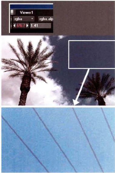
Figure 8.30. (Top) Gain controls. The f-stop is indicated by the red f/n value. The Gain value appears to the right of the F-stop arrows. (Center) Footage with banding area indicated by box. (Bottom) Detail of banding revealed with adjusted Gain value. The band transitions are indicated by the gray lines.
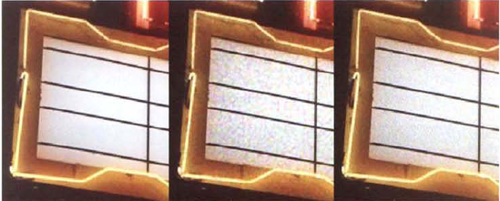
To disguise the color banding, you can add a blur. With the Shuffle1 node selected, RMB+click and choose Filter → Blur. In the Blur1 node's properties panel, set the Size slider to 12. A heavy blur is added to the footage, which hides the banding in the sky. However, the trees and clouds are equally blurred.
To restore sharpness to the foreground, you can mask the blurred sky and merge it with an unblurred copy of the footage. With no nodes selected, choose Draw → Bezier. With the Bezier1 node's properties panel open, Crtl+Alt+click in the viewer to draw a mask. In the Bezier1 node's properties panel, set Extra Blur to 40. With node nodes selected, RMB+click and choose Merge → Merge. Connect the output of the Blur1 node to input A of the Merge1 node (see Figure 8.31). Connect the Mask input of the Merge1 node to the output of the Bezier1 node. Connect a viewer to the Merge1 node. The blurred sky is cut out by the mask (see Figure 8.31). Connect the output of the Shuffle1 node to input B of the Merge1 node. The masked, blurred portion of the sky is placed on top of an unaffected version of the footage.
Although the color banding is significantly reduced, the sky has lost its inherent noise. To add noise, choose the Blur1 node, RMB+click, and choose Draw → Grain. A Grain1 node is inserted between the Blur1 and Merge1 nodes. Open the Grain1 node's properties panel. Reduce the Size Red, Green, and Blue sliders to values between 5 and 10. Reduce the Intensity Red, Green, and Blue sliders to values between 0.05 and 0.1. Play back the timeline. By default, the grain changes its pattern over time. If the grain remains too heavy, slowly reduce the Intensity values. The tutorial is complete. An example Nuke script is saved as
nuke9.nkin the Tutorials folder on the DVD.

Shawn Jones began his career as a director of photography in the early 1990s. He transitioned to audio engineering when he was hired by Sony Electronics to help develop the Sony Dynamic Digital Sound (SDDS) format. In 1996, he joined NT. In 2007, he received an Academy Award in the scientific and technical category for the Environmental Film Initiative, an industry-wide effort to eliminate silver from 35mm film release prints. At present, Shawn serves as chief technology officer for NT and is the studio's resident colorist.
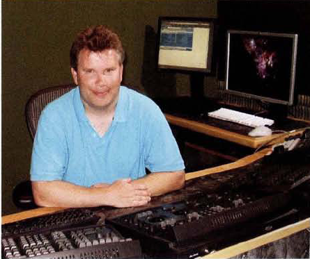
Shawn Jones at a Da Vinci Resolve color grading station
NT Picture & Sound is a division of NT, a studio with 30 years experience in the fine art of optical soundtrack mastering, film scanning and recording, and sound transfer. The NT Picture & Sound facility in Hollywood offers color grading, conforming, and DI services. NT has contributed to such recent feature films as Watchmen, Star Trek, Inglourious Basterds, District 9, and Angels & Demons.
LL: What is the practical goal of color grading?
SJ: In general, you're simply trying to eliminate the bumps that occurred [during] the production.... You're trying to do the same thing with photo-chemical developing—you're just trying to smooth out what you were given for that particular day [of the shoot]. My direction is to [color balance] the faces.... As long as nothing jumps out at you, that's the starting point. From there, you're [working on] the director's intent—darker, lighter, warmer, colder...and then playing with power windows (masked areas of a frame)....
LL: How critical is color grading to a project?
SJ: A general audience will not notice the subtle things that you've done, but they'll notice anything gross that you've missed. So, you're really just trying to smooth out the deficiencies in the original material.... No matter what show I've [worked on], the director of photography has always botched something for whatever reason—it's not usually their fault—they had a bad day, the sun went down, somebody put the wrong gel on the light....
LL: What color grading system is used at NT?
SJ: Da Vinci Resolve.... We also have [Assimilate] Scratch and Color from Apple.
The NT sign at the studio's Hollywood facility
LL: What image format do you use for color grading?
SJ: 10-bit DPX. It's all log. Sometimes, on some of the effects work, it will be 16-bit linear [TIFFs]....
LL: So, you'll play back 10-bit log files in real time?
SJ: Yes, with a film LUT or a video LUT.
LL: How do you manage your color calibration?
SJ: We use cineSpace as our color engine at the moment with some modifications that we've done.... Every day that we're [color grading], the projector's calibrated-it's a continual process. If it drifts a little, you're screwed.
LL: How often do you update your LUTs?
SJ: The [output quality of a film developing lab] yo-yos every day, but on a whole it's pretty consistent.... What varies is the bulb in the projector, the DLP chip as it heats up-from day to day, that changes...so our LUTs get updated based more on what happens in the room and the environment than on what happens on the film.
LL: Do you use multiple LUTs for different displays?
SJ: Every device has its own LUT. [We use cineSpace] to do the profiling and LUT creation.
LL: What's the main advantage of a 3D LUT over a 1D LUT?
SJ: If you're trying to emulate film, it's the only way you can do it.... The only reason you really need a 3D LUT is the [color] cross-talk....
LL: Any other advantages of a 3D LUT?
SJ: A 3D LUT allows you to translate between differing devices with different gamuts. You can soft-clip the variance a little bit better. A blue that's clipping in a video [color] space that doesn't clip in the film [color] space, [can be soft-clipped]...at least you can roll into it (that is, you can gradually transition to the clipped values)....
LL: What resolutions do you work at?
SJ: It's gone from SD to 4K. It really depends on the job. We've done a few 6K elements.
