
Chapter 17. Fragment Shading: Empower Your Pixel Processing
WHAT YOU’LL LEARN IN THIS CHAPTER:
• How to light an object per-fragment
• How to perform procedural texture mapping
As you may recall from Chapter 15, “Programmable Pipeline: This Isn’t Your Father’s OpenGL,” fragment shaders replace the texturing, color sum, and fog stages of the fixed functionality pipeline. This is the section of the pipeline where the party is happening. Instead of marching along like a mindless herd of cattle, applying each enabled texture based on its preordained texture coordinate, your fragments are free to choose their own adventure. Mix and match textures and texture coordinates. Or calculate your own texture coordinates. Or don’t do any texturing, and just compute your own colors. It’s all good.
In their natural habitat, vertex shaders and fragment shaders are most often mated for life. Fragment shaders are the dominant partner, directly producing the eye candy you see displayed on the screen, and thus they receive the most attention. However, vertex shaders play an important supporting role. Because they tend to be executed much less frequently (except for the smallest of triangles), as much of the grunt work as possible is pushed into the vertex shader in the name of performance. The results are then placed into interpolants for use as input by the fragment shader. The vertex shader is a selfless producer, the fragment shader a greedy consumer.
In this chapter, we continue the learning by example we began in the preceding chapter. We present many fragment shaders, both as further exposure to the OpenGL Shading Language (GLSL) and as a launch pad for your own future dabbling. Because you rarely see fragment shaders alone, after you get the hang of fragment shaders in isolation, we will move on to discuss several examples of vertex shaders and fragment shaders working together in peaceful harmony.
Color Conversion
We almost have to contrive some examples illustrating where fragment shaders are used without vertex shader assistance. But we can easily separate them where we simply want to alter the existing color. For these examples, we use fixed functionality lighting to provide a starting color. Then we go to town on it.
Grayscale
One thing you might want to do in your own work is simulate black-and-white film. Given the incoming red, green, and blue color channel intensities, we would like to calculate a single grayscale intensity to output to all three channels. Red, green, and blue each reflect light differently, which we represent by their different contributions to the final intensity. The weights used in our shader derive from the NTSC standard for converting color television signals for viewing on black and white televisions.
Figure 17.1 shows the vertex shader corresponding to Listing 17.1. This may be the only black-and-white figure in the book that is truly supposed to be black-and-white!
Figure 17.1. This fragment shader converts the RGB color into a single grayscale value.
Listing 17.1. Grayscale Conversion Fragment Shader
// grayscale.fs
//
// convert RGB to grayscale
void main(void)
{
// Convert to grayscale using NTSC conversion weights
float gray = dot(gl_Color.rgb, vec3(0.299, 0.587, 0.114));
// replicate grayscale to RGB components
gl_FragColor = vec4(gray, gray, gray, 1.0);
}
The key to all these fragment shaders is that what you write to the color output, gl_FragColor, is what is passed along down the rest of the OpenGL pipeline, eventually to the framebuffer. The primary color input is gl_Color.
Try playing with the contributions of each color channel. Notice how they add up to 1. You can simulate overexposure by making them add up to more than 1, and less than 1 will simulate underexposure.
Sepia Tone
In this next example, we recolorize the grayscale picture with a sepia tone. This tone gives the picture the tint of an Old West photograph. To do this, we first convert to grayscale as before. Then we multiply the gray value by a color vector, which accentuates some color channels and reduces others. Listing 17.2 illustrates this sepia-tone conversion, and the result is as shown in Color Plate 15.
Listing 17.2. Sepia-Tone Conversion Fragment Shader
// sepia.fs
//
// convert RGB to sepia tone
void main(void)
{
// Convert RGB to grayscale using NTSC conversion weights
float gray = dot(gl_Color.rgb, vec3(0.299, 0.587, 0.114));
// convert grayscale to sepia
gl_FragColor = vec4(gray * vec3(1.2, 1.0, 0.8), 1.0);
}
You can choose to colorize with any tint you like. Go ahead and play with the tint factors. Here, we’ve hard-coded one for sepia. If you’re truly ambitious, you could substitute external application-defined uniform constants to make the tint color user-selectable so that you don’t have to write a different shader for every tint color.
Inversion
For this next example, we’re going for the film negative effect. These shaders are almost too simple to mention. All you have to do is take whatever color you were otherwise going to draw and subtract that color from 1. Black becomes white, and white becomes black. Red becomes cyan. Purple becomes chartreuse. You get the picture.
Figure 17.2 illustrates the color inversion performed in Listing 17.3. Use your imagination or consult the sample code for the grayscale inversion, which is just as straightforward.
Figure 17.2. This fragment shader inverts the RGB color, yielding a film negative effect.
Listing 17.3. Color Inversion Fragment Shader
// colorinvert.fs
//
// invert like a color negative
void main(void)
{
// invert color components
gl_FragColor.rgb = 1.0 - gl_Color.rgb;
gl_FragColor.a = 1.0;
}
Heat Signature
Now, we attempt our first texture lookup. In this sample shader, we simulate a heat signature effect like the one in the movie Predator. Heat is represented by a color spectrum ranging from black to blue to green to yellow to red.
We again use the grayscale conversion, this time as our scalar heat value. This is a cheap trick for demonstration purposes, as the color intensity does not necessarily have any relationship to heat. In reality, the heat value would be passed in as a separate vertex attribute or uniform. We use this value as a texture coordinate to index into a 1D texture populated with the color gradients from black to red. Figure 17.3 shows the results of the heat signature shader in Listing 17.4.
Figure 17.3. This fragment shader simulates a heat signature by looking up a color from a 1D texture. (This figure also appears in the Color insert.)

Listing 17.4. Heat Signature Fragment Shader
// heatsig.fs
//
// map grayscale to heat signature
uniform sampler1D sampler0;
void main(void)
{
// Convert to grayscale using NTSC conversion weights
float gray = dot(gl_Color.rgb, vec3(0.299, 0.587, 0.114));
// look up heatsig value
gl_FragColor = texture1D(sampler0, gray);
}
Dependent Texture Lookups
Fixed functionality texture mapping was very strict, requiring all texture lookups to use an interpolated per-vertex texture coordinate. One of the powerful new capabilities made possible by fragment shaders is that you can calculate your own texture coordinates per-fragment. You can even use the result of one texture lookup as the coordinate for another lookup. All these cases are considered dependent texture lookups. They’re named that because the lookups are dependent on other preceding operations in the fragment shader.
You may not have noticed, but we just performed a dependent texture lookup in the heat signature shader. First, we had to compute our texture coordinate by doing the grayscale conversion. Then we used that value as a texture coordinate to perform a dependent texture lookup into the 1D heat signature texture.
The dependency chain can continue: You could, for example, take the color from the heat signature shader and use that as a texture coordinate to perform a lookup from a cube map texture, perhaps to gamma-correct your color. Beware, however, that some OpenGL implementations have a hardware limit as to the length of dependency chains, so keep this point in mind if you want to avoid falling into a non-hardware-accelerated driver path!
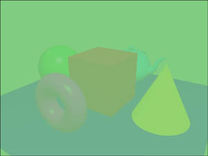
Per-Fragment Fog
Instead of performing fog blending per-vertex, or calculating the fog factor per-vertex and using fixed functionality fog blending, we compute the fog factor and perform the blend ourselves within the fragment shader in the following example. This example emulates GL_EXP2 fog mode except that it will be more accurate than most fixed functionality implementations, which apply the exponentiation per-vertex instead of per-fragment.
This is most noticeable on low-tessellation geometry that extends from the foreground to the background, such as the floor upon which all the objects in the scene rest. Compare the results of this shader with the fog shaders in the preceding chapter, and you can readily see the difference.
Figure 17.4 illustrates the output of the fog shader in Listing 17.5.
Figure 17.4. This fragment shader performs per-fragment fog computation.
Listing 17.5. Per-Fragment Fog Fragment Shader
// fog.fs
//
// per-pixel fog
uniform float density;
void main(void)
{
const vec4 fogColor = vec4(0.5, 0.8, 0.5, 1.0);
// calculate 2nd order exponential fog factor
// based on fragment's Z distance
const float e = 2.71828;
float fogFactor = (density * gl_FragCoord.z);
fogFactor *= fogFactor;
fogFactor = clamp(pow(e, -fogFactor), 0.0, 1.0);
// Blend fog color with incoming color
gl_FragColor = mix(fogColor, gl_Color, fogFactor);
}
We need to comment on a few things here. One is the built-in function used to blend: mix. This function blends two variables of any type, in this case four-component vectors, based on the third argument, which should be in the range [0,1].
Another thing to notice is how we have chosen to make the density an externally set uniform constant rather than a hard-coded inline constant. This way, we can tie the density to keystrokes. When the user hits the left or right arrows, we update the density shader constant with a new value without having to change the shader text at all. As a general rule, constant values that you may want to change at some point should not be hard-coded, but all others should be. By hard-coding a value, you give the OpenGL implementation’s optimizing compiler an early opportunity to use this information to possibly make your shader run even faster.
Image Processing
Image processing is another application of fragment shaders that doesn’t depend on vertex shader assistance. After drawing the scene without fragment shaders, we can apply convolution kernels to post-process the image in various ways.
To keep the shaders concise and improve the probability of their being hardware-accelerated on a wider range of hardware, we’ve limited the kernel size to 3×3. Feel free to experiment with larger kernel sizes.
Within the sample application, glCopyTexImage2D is called to copy the contents of the framebuffer into a texture. The texture size is chosen to be the largest power-of-two size smaller than the window. (If OpenGL 2.0 or the ARB_texture_non_power_of_two extension is supported, the texture can be the same size as the window.) A fragment-shaded quad is then drawn centered within the window with the same dimensions as the texture, with a base texture coordinate ranging from (0,0) in the lower left to (1,1) in the upper right.
The fragment shader takes its base texture coordinate and performs a texture lookup to obtain the center sample of the 3×3 kernel neighborhood. It then proceeds to apply eight different offsets to look up samples for the other eight spots in the neighborhood. Finally, the shader applies some filter to the neighborhood to yield a new color for the center of the neighborhood. Each sample shader provides a different filter commonly used for image-processing tasks.
Blur
Blurring may be the most commonly applied filter in everyday use. It smoothes out high-frequency features, such as the jaggies along object edges. It is also called a low-pass filter because it lets low-frequency features pass through while filtering out high-frequency features.
Because we’re using only a 3×3 kernel, the blur is not overly dramatic in a single pass. We could make it more blurry by using a larger kernel or by applying the blur filter multiple times in successive passes. Figure 17.5 shows the results of the blur filter in Listing 17.6 after five passes.
Figure 17.5. This fragment shader blurs the scene. (This figure also appears in the Color insert.)

Listing 17.6. Post-Process Blur Fragment Shader
// blur.fs
//
// blur (low-pass) 3x3 kernel
uniform sampler2D sampler0;
uniform vec2 tc_offset[9];
void main(void)
{
vec4 sample[9];
for (int i = 0; i < 9; i++)
{
sample[i] = texture2D(sampler0,
gl_TexCoord[0].st + tc_offset[i]);
}
// 1 2 1
// 2 1 2 / 13
// 1 2 1
gl_FragColor = (sample[0] + (2.0*sample[1]) + sample[2] +
(2.0*sample[3]) + sample[4] + (2.0*sample[5]) +
sample[6] + (2.0*sample[7]) + sample[8]) / 13.0;
}
The first thing we do in the blur shader is generate our nine texture coordinates. This is accomplished by adding precomputed constant offsets to the interpolated base texture coordinate. The offsets were computed taking into account the size of the texture such that the neighboring texels to the north, south, east, west, northeast, southeast, northwest, and southwest could be obtained by a simple 2D texture lookup.
This neighborhood is obtained the same way in all our image processing shaders. It is the filter applied to the neighborhood that differs in each shader. In the case of the blur filter, the texel neighborhood is multiplied by a 3×3 kernel of coefficients (1s and 2s), which add up to 13. The resulting values are all summed and averaged by dividing by 13, resulting in the new color for the texel. Note that we could have made the kernel coefficient values 1/13 and 2/13 instead of 1 and 2, but that would have required many extra multiplies. It is simpler and cheaper for us to factor out the 1/13 and just apply it at the end.
Try experimenting with the filter coefficients. What if, for example, you put a weight of 1 at each corner and then divide by 4? Notice what happens when you divide by more or less than the sum of the coefficients: The scene grows darker or lighter. That makes sense. If your scene was all white, you would be effectively multiplying the filter coefficients by 1 and adding them up. If you don’t divide by the sum of the coefficients, you’ll end up with a color other than white.
Sharpen
Sharpening is the opposite of blurring. Some examples of its use include making edges more pronounced and making text more readable. Figure 17.6 illustrates the use of sharpening, applying the filter in two passes.
Figure 17.6. This fragment shader sharpens the scene. (This figure also appears in the Color insert.)

Here is the shader code for applying the sharpen filter:
// sharpen.fs
//
// 3x3 sharpen kernel
uniform sampler2D sampler0;
uniform vec2 tc_offset[9];
void main(void)
{
vec4 sample[9];
for (int i = 0; i < 9; i++)
{
sample[i] = texture2D(sampler0,
gl_TexCoord[0].st + tc_offset[i]);
}
// -1 -1 -1
// -1 9 -1
// -1 -1 -1
gl_FragColor = (sample[4] * 9.0) -
(sample[0] + sample[1] + sample[2] +
sample[3] + sample[5] +
sample[6] + sample[7] + sample[8]);
}
Notice how this kernel also sums to 1, as did the blur filter. This operation guarantees that, on average, the filter is not increasing or decreasing the brightness. It’s just sharpening the brightness, as desired.
Dilation and Erosion
Dilation and erosion are morphological filters, meaning they alter the shape of objects. Dilation grows the size of bright objects, whereas erosion shrinks the size of bright objects. (They each have the reverse effect on dark objects.) Figures 17.7 and 17.8 show the effects of three passes of dilation and erosion, respectively.
Figure 17.7. This fragment shader dilates objects.
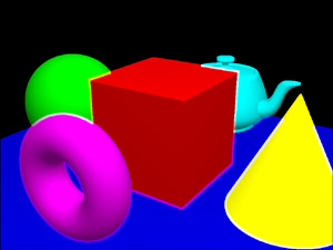
Figure 17.8. This fragment shader erodes objects.

Dilation simply finds the maximum value in the neighborhood:
// dilation.fs
//
// maximum of 3x3 kernel
uniform sampler2D sampler0;
uniform vec2 tc_offset[9];
void main(void)
{
vec4 sample[9];
vec4 maxValue = vec4(0.0);
for (int i = 0; i < 9; i++)
{
sample[i] = texture2D(sampler0,
gl_TexCoord[0].st + tc_offset[i]);
maxValue = max(sample[i], maxValue);
}
gl_FragColor = maxValue;
}
Erosion conversely finds the minimum value in the neighborhood:
// erosion. fs
//
// minimum of 3x3 kernel
uniform sampler2D sampler0;
uniform vec2 tc_offset[9];
void main(void)
{
vec4 sample[9];
vec4 minValue = vec4(1.0);
for (int i = 0; i < 9; i++)
{
sample[i] = texture2D(sampler0,
gl_TexCoord[0].st + tc_offset[i]);
minValue = min(sample[i], minValue);
}
gl_FragColor = minValue;
}
Edge Detection
One last filter class worthy of mention here is edge detectors. They do just what you would expect—detect edges. Edges are simply places in an image where the color changes rapidly, and edge detection filters pick up on these rapid changes and highlight them.
Three widely used edge detectors are Laplacian, Sobel, and Prewitt. Sobel and Prewitt are gradient filters that detect changes in the first derivative of each color channel’s intensity, but only in a single direction. Laplacian, on the other hand, detects zero-crossings of the second derivative, where the intensity gradient suddenly changes from getting darker to getting lighter, or vice versa. It works for edges of any orientation.
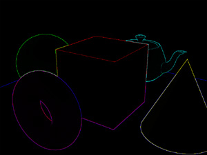
Because the differences in their results are subtle, Figure 17.9 shows the results from only one of them, the Laplacian filter. Try out the others and examine their shaders at your leisure in the accompanying sample code.
Figure 17.9. This fragment shader implements Laplacian edge detection. (This figure also appears in the Color insert.)
The Laplacian filter code is almost identical to the sharpen code we just looked at:
// laplacian.fs
//
// Laplacian edge detection
uniform sampler2D sampler0;
uniform vec2 tc_offset[9];
void main(void)
{
vec4 sample[9];
for (int i = 0; i < 9; i++)
{
sample[i] = texture2D(sampler0,
gl_TexCoord[0].st + tc_offset[i]);
}
// -1 -1 -1
// -1 8 -1
// -1 -1 -1
gl_FragColor = (sample[4] * 8.0) -
(sample[0] + sample[1] + sample[2] +
sample[3] + sample[5] +
sample[6] + sample[7] + sample[8]);
}
The difference, of course, is that the center kernel value is 8 rather than the 9 present in the sharpen kernel. The coefficients sum up to 0 rather than 1. This explains the blackness of the image. Instead of, on average, retaining its original brightness, the edge detection kernel will produce 0 in areas of the image with no color change.
Lighting
Welcome back to another discussion of lighting shaders. In the preceding chapter, we covered per-vertex lighting. We also described a couple of per-fragment fixed functionality tricks to improve the per-vertex results: separate specular with color sum and power function texture for specular exponent. In this chapter, we perform all our lighting calculations in the fragment shader to obtain the greatest accuracy.
The shaders here will look very familiar. The same lighting equations are implemented, so the code is virtually identical. One new thing is the use of vertex shaders and fragment shaders together. The vertex shader sets up the data that needs to be interpolated across the line or triangle, such as normals and light vectors. The fragment shader then proceeds to do most of the work, resulting in a final color.
Diffuse Lighting
As a refresher, the equation for diffuse lighting follows:
Cdiff = max{N • L, 0} * Cmat * Cli
You need a vertex shader that generates both normal and light vectors. Listing 17.7 contains the vertex shader source to generate these necessary interpolants for diffuse lighting.
Listing 17.7. Diffuse Lighting Interpolant Generating Vertex Shader
// diffuse.vs
//
// set up interpolants for diffuse lighting
uniform vec3 lightPos0;
varying vec3 N, L;
void main(void)
{
// vertex MVP transform
gl_Position = gl_ModelViewProjectionMatrix * gl_Vertex;
// eye-space normal
N = gl_NormalMatrix * gl_Normal;
// eye-space light vector
vec4 V = gl_ModelViewMatrix * gl_Vertex;
L = lightPos0 - V.xyz;
// Copy the primary color
gl_FrontColor = gl_Color;
}
Notice how we are able to give descriptive names N and L to our interpolants, known as varyings. They have to match the names used in the fragment shader. All in all, this feature makes the shaders much more readable and less error prone than if we were using generic texture coordinate interpolants. For example, if we weren’t careful, we might accidentally output L into texture coordinate 0, whereas the fragment shader is expecting it in texture coordinate 1. No compile error would be thrown. GLSL matches up our custom varyings automatically by name, keeping us out of trouble and at the same time avoiding the need for tedious comments in code explaining the contents of each interpolant.
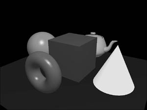
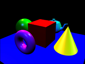
The diffuse lighting fragment shaders resulting in Figure 17.10 follow in Listing 17.8. Unlike colors produced by specular lighting, diffuse lit colors do not change rapidly across a line or triangle, so you will probably not be able to distinguish between per-vertex and per-fragment diffuse lighting. For this reason, in general, it would be more efficient to perform diffuse lighting in the vertex shader, as we did in the preceding chapter. We perform it here per-fragment simply as a learning exercise.
Figure 17.10. Per-fragment diffuse lighting.
Listing 17.8. Diffuse Lighting Fragment Shader
// diffuse.fs
//
// per-pixel diffuse lighting
varying vec3 N, L;
void main(void)
{
// output the diffuse color
float intensity = max(0.0,
dot(normalize(N), normalize(L)));
gl_FragColor = gl_Color;
gl_FragColor.rgb *= intensity;
}
First, we normalize the interpolated normal and light vectors. Then one more dot product, a clamp, and a multiply, and we’re finished. Because we want a white light, we can save ourselves the additional multiply by Cli = {1,1,1,1}.
Multiple Specular Lights
Rather than covering specular lighting and multiple light samples independently, we’ll cover both at the same time. As a refresher, the specular lighting equation is
Cspec= max{N • H, 0}Sexp * Cmat * Cli
The vertex shader needs to generate light vector interpolants for all three lights, in addition to the normal vector. We’ll calculate the half-angle vector in the fragment shader. Listing 17.9 shows the vertex shader for the three diffuse and specular lights.
Listing 17.9. Three Lights Vertex Shader
// 3lights.vs
//
// set up interpolants for 3 specular lights
uniform vec3 lightPos[3];
varying vec3 N, L[3];
void main(void)
{
// vertex MVP transform
gl_Position = gl_ModelViewProjectionMatrix * gl_Vertex;
vec4 V = gl_ModelViewMatrix * gl_Vertex;
// eye-space normal
N = gl_NormalMatrix * gl_Normal;
// Light vectors
for (int i = 0; i < 3; i++)
L[i] = lightPos[i] - V.xyz;
// Copy the primary color
gl_FrontColor = gl_Color;
}
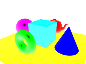
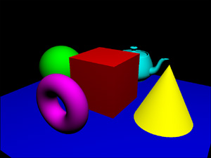
The fragment shaders will be doing most of the heavy lifting. Figure 17.11 shows the result of Listing 17.10.
Figure 17.11. Per-fragment diffuse and specular lighting with three lights.
Listing 17.10. Three Diffuse and Specular Lights Fragment Shader
// 3lights.fs
//
// 3 specular lights
varying vec3 N, L[3];
void main(void)
{
const float specularExp = 128.0;
vec3 NN = normalize(N);
// Light colors
vec3 lightCol[3];
lightCol[0] = vec3(1.0, 0.25, 0.25);
lightCol[1] = vec3(0.25, 1.0, 0.25);
lightCol[2] = vec3(0.25, 0.25, 1.0);
gl_FragColor = vec4(0.0);
for (int i = 0; i < 3; i++)
{
vec3 NL = normalize(L[i]);
vec3 NH = normalize(NL + vec3(0.0, 0.0, 1.0));
float NdotL = max(0.0, dot(NN, NL));
// Accumulate the diffuse contributions
gl_FragColor.rgb += gl_Color.rgb * lightCol[i] *
NdotL;
// Accumulate the specular contributions
if (NdotL > 0.0)
gl_FragColor.rgb += lightCol[i] *
pow(max(0.0, dot(NN, NH)), specularExp);
}
gl_FragColor.a = gl_Color.a;
}
This time, we made each of the three lights a different color instead of white, necessitating an additional multiply by lightCol[n](Cli).
Procedural Texture Mapping
When can you texture map an object without using any textures? When you’re using procedural texture maps. This technique enables you to apply colors or other surface properties to an object, just like using conventional texture maps. With conventional texture maps, you load a texture image into OpenGL with glTexImage; then you perform a texture lookup within your fragment shader. However, with procedural texture mapping, you skip the texture loading and texture lookup and instead describe algorithmically what the texture looks like.
Procedural texture mapping has advantages and disadvantages. One advantage is that its storage requirements are measured in terms of a few shader instructions rather than megabytes of texture cache and/or system memory consumed by conventional textures. This frees your storage for other uses, such as vertex buffer objects, discussed in Chapter 11, “It’s All About the Pipeline: Faster Geometry Throughput,” or some of the advanced buffers discussed in the next chapter.
Another benefit is its virtually limitless resolution. Like vector drawing versus raster drawing, procedural textures scale to any size without loss of quality. Conventional textures require you to increase texture image sizes to improve quality when greatly magnified. Eventually, you’ll hit a hardware limit. The only hardware limit affecting procedural texture quality is the floating-point precision of the shader processors, which are required to be at least 24-bit for OpenGL.
A disadvantage of procedural texture maps, and the reason they’re not used more frequently, is that the complexity of the texture you want to represent requires an equally complex fragment shader. Everything from simple shapes and colors all the way to complex plasma, fire, smoke, marble, or wood grain can be achieved with procedural textures, given enough shader instructions to work with. But sometimes you just want the company logo or a satellite map or someone’s face textured onto your scene. Certainly, conventional textures will always serve a purpose!
Checkerboard Texture
Enough discussion. Let’s warm up with our first procedural texture: a 3D checkerboard. Our object will appear to be cut out of a block of alternating white and black cubes. Sounds simple enough, right?
We’ll use the object-space position at each fragment to decide what color to make that fragment. So we need a vertex shader that, in addition to transforming the object-space position to clip-space as usual, also copies that object-space position into an interpolant so that it becomes available to the fragment shader. While we’re at it, we might as well add diffuse and specular lighting, so our vertex shader needs to output the normal and light vector as well.
Listing 17.11 shows the vertex shader. We’ll use it for all three of our procedural texture mapping examples.
Listing 17.11. Procedural Texture Mapping Vertex Shader
// checkerboard.vs
//
// Generic vertex transformation,
// copy object-space position and
// lighting vectors out to interpolants
uniform vec3 lightPos;
varying vec3 N, L, V;
void main(void)
{
// normal MVP transform
gl_Position = gl_ModelViewProjectionMatrix * gl_Vertex;
// map object-space position onto unit sphere
V = gl_Vertex.xyz;
// eye-space normal
N = gl_NormalMatrix * gl_Normal;
// eye-space light vector
vec4 Veye = gl_ModelViewMatrix * gl_Vertex;
L = lightPos - Veye.xyz;
}
The object we’re using for our examples is a sphere. The size of the sphere doesn’t matter because we normalize the object-space position at the beginning of the fragment shader. This means that all the positions we deal with in the fragment shader will be in the range [–1,1].
Our strategy for the fragment shader will be to break up the range [–1,1] into eight alternating blocks along each axis. Each block will be assigned an alternating value of 0 or 1 for each axis, as illustrated in Figure 17.12. If the total of the three values is even, we paint it black; otherwise, we paint it white.
Figure 17.12. This diagram illustrates how we assign alternating colors to blocks of fragments.
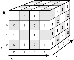
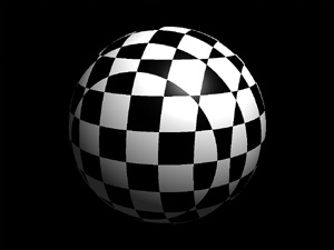
Figure 17.13 shows the result of Listing 17.12, which implements our checkerboard procedural texture mapping algorithm.
Figure 17.13. This 3D checkerboard is generated without using any texture images.
Listing 17.12. Checkerboard Fragment Shader

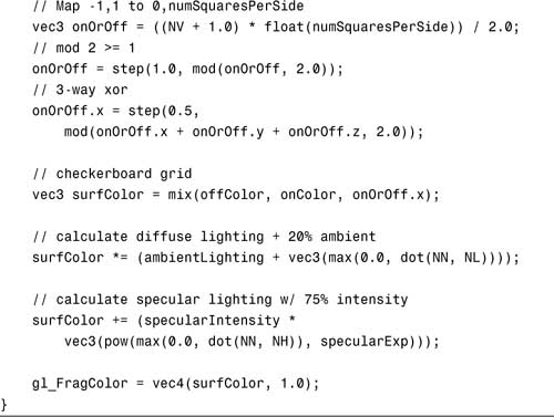
GLSL has a built-in modulo function, mod, which is used to achieve the alternating blocks. Next, we must determine whether the value is within [0,1] or [1,2]. We do this using the step function, which returns 1 if the second argument is greater than or equal to the first, and 0 otherwise.
Now that we have a value of 0 or 1 on each axis, we sum those three values and again perform modulo 2 and a greater-than-or-equal-to comparison. That way, we can assign colors of black or white based on whether the final sum is even or odd. We accomplish this with mix.
You can very easily alter the shaders to change the checkerboard colors or to adjust the number of blocks per row. Give it a try!
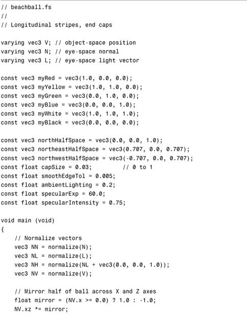
Beach Ball Texture
In this next sample, we’re going to turn our sphere into a beach ball. The ball will have eight longitudinal stripes with alternating primary colors. The north and south poles of the ball will be painted white. Let’s get started!
Look at the ball from above. We’ll be slicing it up into three half spaces: north-south, northeast-southwest, and northwest-southeast. See Figure 17.14 for a visual depiction. The north slices are assigned full red values, and south slices are assigned no red. The two slices that are both in the southeast half space and the northeast half space are assigned full green, and all other slices receive no green. Notice how the overlapping red and green slice becomes yellow. Finally, all slices in the southwest half space are assigned the color blue.
Figure 17.14. An overhead view showing how the beach ball colors are assigned. (This figure also appears in the Color insert.)
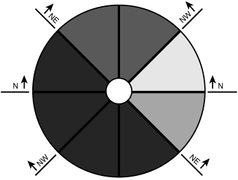
The east slices nicely alternate from red to yellow to green to blue. But what about the west slices? The easiest way to address them is to effectively copy the east slices and rotate them 180 degrees. We’re looking down at the ball from the positive y-axis. If the object-space position’s x coordinate is greater than or equal to 0, the position is used as-is. However, if the coordinate is less than 0, we negate both the x-axis and z-axis positions, which maps the original position to its mirror on the opposite side of the beach ball.
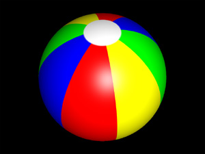
The white caps at the poles are simple to add in. After coloring the rest of the ball with stripes, we replace that color with white whenever the absolute value of the y-axis position is close to 1. Figure 17.15 shows the result of the beach ball shaders in Listing 17.13.
Figure 17.15. You have built your own beach ball from scratch! (This figure also appears in the Color insert.)
Listing 17.13. Beach Ball Fragment Shader

After remapping all negative x positions as described earlier, we use dot products to determine on which side of each half space the current object-space coordinate falls. The sign of the dot product tells us which side of the half space is in play.
Notice we don’t use the built-in step function this time. Instead, we introduce a new and improved version: smoothstep. Instead of transitioning directly from 0 to 1 at the edge of a half space, smoothstep allows for a smooth transition near the edge where values between 0 and 1 are returned. Switch back and forth between step and smoothstep and you’ll see how it helps reduce the aliasing jaggies.
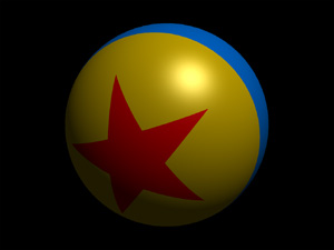
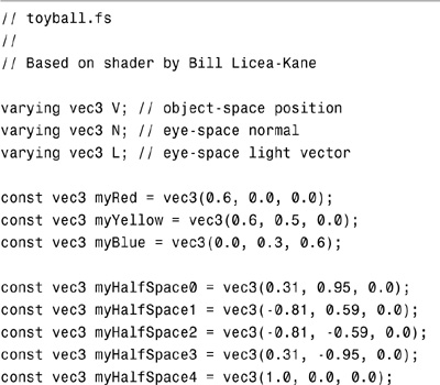
Toy Ball Texture
For our final procedural texture mapping feat, we’ll transform our sphere into a familiar toy ball, again using no conventional texture images. This ball will have a red star on a yellow background circumscribed by a blue stripe. We will describe all this inside a fragment shader.
The tricky part is obviously the star shape. For each fragment, the shader must determine whether the fragment is within the star, in which case it’s painted red, or whether it remains outside the star, in which case it’s painted yellow. To make this determination, we first detect whether the fragment is inside or outside five different half spaces, as shown in Figure 17.16.
Figure 17.16. This diagram illustrates the determination of whether a fragment is inside or outside the star.

Any fragment that is inside at least four of the five half spaces is inside the star. We’ll start a counter at –3 and increment it for every half space that the fragment falls within. Then we’ll clamp it to the range [0,1]. A 0 indicates that we’re outside the star and should paint the fragment yellow. A 1 indicates that we’re inside the star and should paint the fragment red.
Adding the blue stripe, like the white caps on the beach ball, is an easy last step. Instead of repainting fragments close to the ends of the ball, we repaint them close to the center, this time along the z-axis. Figure 17.17 illustrates the result of the toy ball shader in Listing 17.14.
Figure 17.17. The toy ball shader describes a relatively complex shape. (This figure also appears in the Color insert.)
Listing 17.14. Toy Ball Fragment Shader


The half spaces cut through the center of the sphere. This is what we wanted for the beach ball, but for the star we need them offset from the center slightly. This is why we add an extra constant distance to the result of the half-space dot products. The larger you make this constant, the larger your star will be.
Again, we use smoothstep when picking between inside and outside. For efficiency, we put the inside/outside results of the first four half spaces into a four-component vector. This way, we can sum the four components with a single four-component dot product against the vector {1,1,1,1}. The fifth half space’s inside/outside value goes into a lonely float and is added to the other four separately because no five-component vector type is available. You could create such a type yourself out of a structure, but you would likely sacrifice performance on most implementations, which natively favor four-component vectors.
If you want to toy with this shader, try this exercise: Convert the star into a six-pointed star by adding another half space and adjusting the existing half-space planes. Prove to yourself how many half spaces your fragments must fall within now to fall within the star, and adjust the myInOut counter’s initial value accordingly.
Summary
The possible applications of vertex and fragment shaders are limited only by your imagination. We’ve introduced a few just to spark your creativity and to provide you with some basic building blocks so that you can easily jump right in and start creating your own shaders. Feel free to take these shaders, hack and slash them beyond recognition, and invent and discover better ways of doing things while you’re at it. Don’t forget the main objective of this book: Make pretty pictures. So get to it!