|
|
|
|
Nuke Interface |
|

Nuke was designed to create digital visual effects on feature films. As such, it carries a robust set of tools that make high-end postproduction available to professional digital artists, independent filmmakers, students, and hobbyists alike. The core of Nuke’s functionality is a system of connected nodes.
Although node manipulation may seem odd to an artist who has mastered layer-based programs, the efficiency and power of nodes comes to light after a basic knowledge is achieved.
This chapter includes the following critical information:
• Overview of interface panes and panels
• Comparison of layer-based and node-based compositing
• Node manipulation, including creation, connection, adjustment, and arrangement
• File importation and output rendering
• Timeline and flipbook playback
Interface Components
By default, Nuke’s main window is divided into three panes: the Viewer pane, the Node Graph/Curve Editor pane, and the Properties Bin/Script Editor pane (Figure 1.1). Any given pane may have more than one tabbed panel. For example, you can switch from the Node Graph panel and Curve Editor panel by clicking the Curve Editor tab. Each pane includes a content menu, as represented by a gray-checkered Content Menu box at the top left of the pane. If you click on the Content Menu box, a pop-up menu opens and displays a set of options you can use to customize the pane.
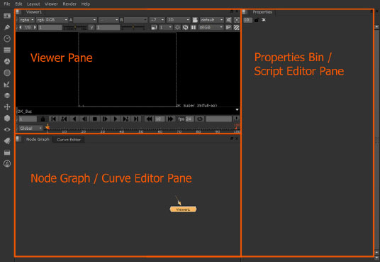
FIGURE 1.1 The three panes of the Nuke window.
The menu bar is located on top left of the Nuke window. The bar hosts commonly used dropdown menus, including File, Edit, and Viewer (Figure 1.2).

FIGURE 1.2 The menu bar, as seen in NukeX 6.3.
The toolbar is located on the left side of the Nuke window and contains between 13 and 17 icons, depending on the version of Nuke you are using. The icons represent different categories of nodes such as Image, Draw, and Time (Figure 1.3). You can use the toolbar to add nodes to the Node Graph. To do so, click on an icon and choose a node from the resulting dropdown menu. It’s also possible to add nodes through an RMB shortcut menu in the Node Graph; this is described in the “Using the Node Graph” section later in this chapter.
Layers Versus Nodes
Adobe After Effects, which is the most widely used compositing package in the world, is layer-based (Figure 1.4). Adobe Photoshop shares a similar layer structure (Figure 1.5).
Nuke, on the other hand, is node-based. A node is a discrete unit used to build linked data structures. On a more basic level, you can think of a node as a box that contains specific information that can be shared with neighboring node boxes. In Nuke, a node is represented by a rectangle icon in the Node Graph (see Figure 1.6 in the next section). The information the node carries is displayed as parameters through its properties panel.
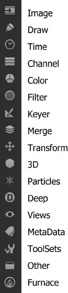
FIGURE 1.3 The toolbar, as seen in NukeX 6.3.
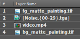
FIGURE 1.4 Adobe After Effects CS5 Timeline with four layers. The lower the layer number, the higher the layer is in the layer stack.
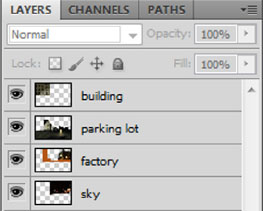
FIGURE 1.5 Adobe Photoshop CS5 Layers window with four layers. The checkered areas within the layer thumbnails represent transparency.
With layer-based compositing, each utilized image sequence, still image, and movie file is placed on a layer. Each layer has its own set transformations and carries an optional set of filters. Layers are stacked and processed in order from bottom to top. This is roughly analogous to a stack of cut-out magazine photos. Higher layers win out over lower layers unless nonstandard blending modes are selected or the higher layers possess transparency. Photoshop PSD files store layer transparency information. Other image formats, such as Targa or TIFF, store transparency through a fourth channel known as alpha.
With node-based compositing, each utilized image sequence, still image, and movie file is represented by a unique node. In Nuke, the Read node fulfills this duty. The output of each Read node is connected to the inputs of other nodes, including various filter nodes and merge nodes. The final result is output to a Viewer node (for display in the program) or a Write node (to write an image sequence to disk).
A Nuke node supports a limited number of inputs. However, you can connect the output of a Nuke node to an unlimited number of nodes. When multiple nodes are connected through their inputs and outputs, the structure is known as a node network, tree graph, process tree, or node graph. In Nuke, the work area that you use to create and edit such node networks is called the Node Graph; the Node Graph can carry multiple networks. More specifically, the node networks are a directed acyclic graph (DAG) where information only flows in one direction for each connection.
There are several advantages to using a node-based compositor:
• You can easily create complex node networks. In contrast, you can only stack layers. With a layer-based system, it’s difficult to connect the output of a single layer to the input of multiple layers; workarounds require the nesting of composites or prerendering certain layers to disk.
• When carefully set up, a node network is easy to interpret. Complex layer-based composites can be difficult to navigate due to the sheer number of layers that are required.
• High-end compositing systems used in the feature animation and visual effects industries are node-based. The systems include Flame, Inferno, Shake, Fusion, and Toxik.
Node Anatomy
Any given node in Nuke has a set of input and output pipes. A pipe is a connection between nodes that allows the flow of information between nodes. A pipe can only send information in one direction. Before a node is connected to another node, the pipes are broken or are indicated by arrow stubs (Figure 1.6).
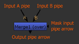
FIGURE 1.6 A Nuke node with input and output pipes. Note that many nodes only possess a single input pipe.
More specifically, a pipe carries one or more channels. A channel is a discrete component of a digital image that represents specific information as scalar values (whereby a pixel of a single channel can only carry in single magnitude or intensity); the information may be the distribution of a primary color, such as red, or the distance an object is from the camera, as with a Z-depth channel. Channels commonly used in Nuke include red, green, and blue (RGB) color channels; alpha channels; Z-depth channels; and U and V direction channels. Thus, a node affects the quality of the channels that pass through the node. That is, the numeric values of the channels are affected by the node. Channels are discussed in more detail in Chapters 3 and 4.
If a node is connected to one or more nodes, Nuke indicates the channels that are flowing through a node by adding small colored lines to the bottom left of the node icon (see Figure 1.18 later in this chapter). If the channel is affected by the node, the line is long. If the channel is unaffected, the line is short. The color coding follows:
Channel |
Color |
Red |
Red |
Green |
Green |
Blue |
Blue |
Alpha |
White |
Z-depth |
Purple |
U |
Pink |
V |
In addition, Nuke indicates the channels a node is affecting by printing a word at the bottom center of the node icon. For example, (red) is printed for the red channel and (all) indicates that all input channels are affected. For information on channel control, see Chapter 4.
Importing Files
To import an image sequence, still image, or movie file, you must create a Read node. To do so, follow these steps:
1. Click the Image icon on the toolbar. Choose Read from the dropdown menu. The File Browser window opens (Figure 1.7).
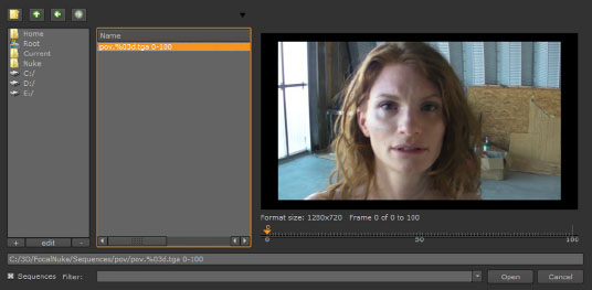
FIGURE 1.7 The File Browser window with the built-in viewer displayed.
2. Navigate to the file you want to open. (For tips on navigation, see the next section.) Once the files are listed in the Pathname field, click the Open button.
3. The File Browser window closes and a Read node is placed in the Node Graph. Nuke numbers new nodes consecutively. To view the imported file, you must connect a Viewer node to the Read node. The Node Graph is provided with a Viewer1 node by default. To make the connection, LMB-drag the dotted 1 pipe extending from the Viewer1 node and drop it on top of the Read1 node (Figure 1.8). The output of the Read1 node is thereby connected to the input of the Viewer1 node through a pipe. Alternatively, you can select the Read node and press the 1 key to automatically connect to Viewer1.
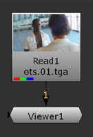
FIGURE 1.8 The Viewer1 node is connected to the output of the Read1 node.
Note that Nuke automatically recognizes numbered image sequences and lists them as under a single name with the format name.placeholder. extension startFrame endFrame. For example, a sequence might appear as name.%02d. tga 1 60 or name.##. tga 1 60. With these examples, the %02d and ## represent the total numeric placeholders, where the original files are named name.01. tga to name.60. tga.
Using the File Browser
The File Browser window offers several ways to navigate the directory structure. The Favorites section features icons for commonly used locations such as the Nuke working directory, system root directory, or various hard drives. To jump to a Favorites location, click the location name so it turns orange. You can add your own Favorites location by navigating to a directory and clicking the + button at the bottom of the Favorites section. To remove a Favorites location, highlight the location in the Favorites section and click the – button. In addition, the window provides Create New Directory, Up One Directory, Previous Directory, and Next Directory buttons at the top left (Figure 1.9). To preview a selected file or image sequence in the File Browser, click the black arrow at the top right. A viewer with playback controls is embedded in the window (see Figure 1.8).

FIGURE 1.9 The File Browser navigation and viewer buttons.
Supported Image Formats
Nuke supports a wide array of image formats. A few of the more commonly used ones are described here.
AVI (.avi). The AVI (Audio Video Interleave) movie format was developed by Microsoft. Nuke’s AVI support is dependent on the FFmpeg open-source audio/video codec library. If an AVI file fails to open, try adding ffmpeg: to the head of the path name (e.g., ffmpeg:C:/Projects/test.avi). For more information on the FFmpeg library, visit ffmpeg.org. On Windows systems, AVI support is also dependent on the DirectShow multimedia framework.
DPX and Cineon (.dpx and .cin). The DPX (Digital Picture Exchange) format is based on the Cineon file format, which was created for Kodak’s early line of digital film scanners. Both formats use a 10-bit log architecture, which is well suited to capture the full exposure range of motion picture film stock. DPX is more flexible than Cineon in that it supports 8-, 12-, 16-, and 32-bit variations that may be linear or log. (Linear and log encoding is described in Chapter 3.)
MayaIFF (.iff). MayaIFF is native to Autodesk Maya. The format has the advantage of supporting alpha, depth, and motion vector channels. Nuke can read MayaIFF but cannot write it.
OpenEXR (.exr). The OpenEXR format was developed by Industrial Light & Magic and is currently available for public use. The format supports linear 16-bit half-float and linear 32-bit floating-point variations. OpenEXR can support an arbitrary number of custom channels, which makes it particularly useful for compositing. OpenEXR is quickly becoming the standard format for animation studios employing floating-point pipelines.
PNG (.png). The PNG (Portable Network Graphics) format was developed to replace the older GIF format. PNG carries an alpha channel and high-quality compression.
QuickTime (.mov). By default, the QuickTime movie format is supported by Windows and Mac OS X operating systems. Linux versions, however, can utilize the QuickTime format through the FFmpeg open-source library. If a QuickTime file fails to open, try adding ffmpeg: to the head of the path name (e.g., ffmpeg:C:/Projects/test.mov).
RAW. RAW image files contain data from the image sensor of a film scanner or DSLR (digital single-lens reflex) camera. Nuke can read a limited number of DSLR camera types.
REDCODE (.r3d). REDCODE is a proprietary format encoded by the Red One and Red EPIC digital video cameras. Because the Red cameras are often used to capture visual effects plates and shoot high-definition television (HDTV) programs and feature films, Nuke’s ability to read the format is currently evolving and expanding.
Targa (.tga). Targa was developed in the 1980s by Truevision. Common variations include 24-bit (8 bits per channel) and 32-bit (8 bits per channel with alpha).
TIFF (.tiff, .tif). The Tagged Image File Format was developed in the 1980s as a means to standardize desktop digital imaging. The format exists with various compression schemes and supports 16-bit and 32-bit floating-point architecture as well as an alpha channel.
Properties Bin
Each node you create is given a properties panel in the Properties Bin pane at the right side of the Nuke window. The properties panels are stacked vertically. Each properties panel carries the node’s unique information—that is, unique parameters. The parameter values are set by string cells (cells that carry text), numeric cells, sliders, or dropdown menus (Figure 1.10). You can close a properties panel at any time by clicking the X button at the top right of the panel title bar. You can reopen a panel for a node by double-clicking the node in the Node Graph.

FIGURE 1.10 The properties panel for a Read node.
Using the Node Graph
The view within the Node Graph is not fixed. You can zoom closer to displayed nodes by scrolling with a middle mouse button (MMB) wheel or Opt/Alt+MMB-dragging. You can move the view left/right or up/down by MMB-dragging. You can automatically center a selected node or nodes by clicking the MMB while the mouse is in the Node Graph.
Creating Nodes
There are several ways to create a new node:
• Click a category icon on the toolbar and choose a node from the dropdown menu.
• RMB-click in the Node Graph and choose a node from the shortcut menu. For example, choose Image > Read (Figure 1.11). This is the method that is most often used in this book.

FIGURE 1.11 RMB node menu available in the Node Graph.
• Press the Tab key while the mouse is in the Node Graph. A shortcut dialog box opens (Figure 1.12). Type the first few letters of the node name. When the node appears in the dropdown menu, click its name.
• A few nodes have default hot keys. For example, pressing the B key while the mouse is in the Node Graph creates a Blur node. R pops up the File Browser window in anticipation of creating a Read node. To see a complete list of hot keys, choose Help > Key Assignments from the menu bar. You can customize the hot key assignments by editing the menu.py Python script; for a demonstration, see Chapter 10.

FIGURE 1.12 Shortcut dialog box activated by the Tab key in the Node Graph.
Connecting, Disconnecting, and Branching Pipes
To connect one node to another, LMB-drag an unconnected pipe and drop it on top of a different node. Nuke automatically distinguishes between inputs and outputs and makes a proper connection (Figure 1.13).

FIGURE 1.13 LMB-dragging an unconnected pipe.
To disconnect a pipe, LMB-drag either end of a pipe away from a node (Figure 1.14). When connected, the arrow end of a pipe is anchored to the input of a node while the nonarrow side of the pipe is anchored to the output of a node.

FIGURE 1.14 Disconnecting a pipe by LMB-dragging the output end.
To branch a node (to make an output go off in two directions), Shift+LMB-drag the arrow (input) side of the pipe and drop it on top of another node (Figure 1.15).
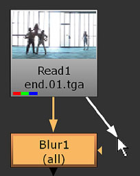
FIGURE 1.15 Branching a pipe by Shift+LMB-dragging the arrow (input) end of the pipe.
Selecting, Moving, Disabling, and Deleting Nodes
You can select a node by clicking it. A selected node turns pale orange. You can select more than one node by Shift-clicking. You can also LMB-drag a selection marquee around multiple nodes. To deselect nodes, simply click an empty area of the Node Graph.
Once a node is selected, you can reposition it within the Node Graph by LMB-dragging. Pipes automatically stretch and shrink to maintain connections.
You can temporarily disable a node by selecting it and pressing the D key. An X is drawn through the node icon (Figure 1.16). When a node is disabled, it has no affect on the input information (it’s as if the node is skipped). To reenable the node, select it and press the D key again. Disabling a node is a good way to see what influence it has on the final output.
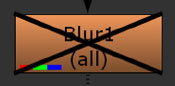
FIGURE 1.16 A disabled node.
To delete a node, press the Delete key while the node is selected.
Creating a Simple Composite
A simple composite includes at least three connected nodes: a Read node, some type of filter node to affect the Read node, and a Viewer node. For example, to apply a Blur node to an imported image, follow these steps:
1. With the mouse in the Node Graph, press the R key. This pops up the File Browser window. Locate an image file. An example file named desert.tif is included in the Chapter1/Bitmaps/ folder on the DVD. Click the Open button.
2. A Read1 node is placed in the Node Graph. LMB-drag the dotted 1 pipe extending from the Viewer1 node and drop it on top of the Read1 node. The output of the Read1 node is thereby connected to the input of the Viewer1 node through a pipe. Alternatively, you can select the Read1 node and press the 1 key to automatically connect to Viewer1. The still image becomes visible in the Viewer1 panel of the Viewer pane. At this point, the image is sharply focused (Figure 1.17).
3. Select the Read1 node. The node turns pale orange. Click the Filter button in the toolbar (it features a solid circle). Choose Blur from the dropdown menu. A Blur1 node is inserted into the network between the Read1 node and the Viewer1 node (Figure 1.18).
4. Initially, there is no change, as the Blur1 node is essentially off by default. To apply a blur, you must raise the Size parameter value. Raise the value by dragging the Value slider, carried by the Blur1 properties panel, to the right (Figure 1.19). (If the properties panel is not visible in the Properties Bin pane, double-click the Blur1 node in the Node Graph.) For example, a Size value of 50 blurs the still significantly (Figure 1.20). The Size parameter determines the size of the convolution filter applied to the image. (Convolution filters are discussed in Chapter 6.)
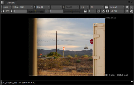
FIGURE 1.17 The imported image, as seen in the Viewer pane.

FIGURE 1.18 A Blur node is added to the node network. Note the red, green, and blue channel lines, as well as the word (all), which indicates that those three channels are affected by the Blur node.

FIGURE 1.19 The Blur1 node properties panel. The Size parameter is set to 50.
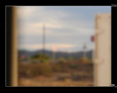
FIGURE 1.20 The result of the network. A sample Nuke script is included as simple_composite.nk in the Chapters/Chapter1/Scripts/ directory on the DVD.
Inserting, Duplicating, and Cloning Nodes
To insert a node into an existing node network, LMB-drag the node and drop it on an existing pipe. The pipe is broken in two and reconnected to the node’s input and output. You can also select an upstream node (one that provides an output) and create a new node through the toolbar. The new node is inserted downstream of the selected node. (The pipe arrows indicate the direction information is flowing; much like water in a river, information in Nuke flows downstream.)
To duplicate a node, select a node and choose Edit > Duplicate from the menu bar or press Opt/Alt+C. The properties of the duplicated node are copied from the original node. If the selected node is part of a node network, the duplicated node is freed from the network and is not connected to any other node.
To clone a node, select a node and choose Edit > Clone from the menu bar or press Opt/Alt+K. The cloned node possesses parameter values that are identical to the original. An orange clone line is drawn between the original and the clone (Figure 1.21). When the original node’s properties are updated, the clone automatically updates to maintain an exact parameter match. If you alter the values of the cloned node, the original node is updated to maintain an exact parameter match.
To make a clone useful, its input and output must be connected to other nodes. For example, in Figure 1.22, a cloned Blur node is used to blur the output of a second Read node. The output of the cloned Blur node is connected to a second Viewer node. You can create additional Viewer nodes at any time by choosing Viewer > Create New Viewer from the menu bar or pressing Ctrl+I.

FIGURE 1.21 A cloned Blur node (right) is connected to the original Blur node (left) via an orange connection line. Both nodes sport a C symbol to further indicate the cloning.

FIGURE 1.22 A cloned Blur node (right) blurs the output of a second Read node. A sample Nuke script is included as blur_clone.nk in the Chapters/Chapter1/Scripts/ directory on the DVD.
Organizing the Node Graph
The Node Graph can quickly become unintelligible if there are a large number of nodes and connections. The following sections contain a few tips for keeping the graph organized.
Snapping and Arranging Nodes
When you LMB-drag a node close to another node in the same node network, the node will vertically or horizontally snap. If you fail to “feel” the snapping action, zoom in closer to the network.
You can select multiple nodes and force Nuke to arrange them in an automatic fashion by pressing the L key.
Creating a Backdrop
You can create a backdrop for a set of nodes. A backdrop is a colored rectangle that distinguishes the node set from other nodes (Figure 1.23). To create a backdrop, select several nodes, RMB-click in the Node Graph, and choose Other > Backdrop. Once you have a backdrop, you can manipulate it in the following ways:
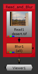
FIGURE 1.23 A backdrop is created for two nodes of a network. The backdrop color is changed from default violet to red. The backdrop is renamed Read_and_Blur.
• You can rename the backdrop by double-clicking its title bar and entering a new name in the name field of its properties panel.
• You can choose your own color for the backdrop by clicking the Tile_color button (to the immediate right of the name field in the properties panel) and selecting a new color from the Color Sliders/Color Wheel dialog box.
• You can resize a backdrop by LMB-dragging the triangular handle at the bottom right corner.
• To move a backdrop, LMB-drag the title bar. Note that any nodes that fall within the interior of the backdrop, whether they are connected to a network or not, are moved along with the backdrop. To move the backdrop without affecting the nodes, Cmd/Ctrl-drag the title bar.
• To delete a backdrop, move all the nodes out of the backdrop area, click the title bar, and press the Delete key.
Bending Pipes
You can create a right-angle bend in a pipe and thus avoid pipes running in a diagonal fashion. To do so, select an upstream node (one that provides the output), RMB-click, and choose Other > Dot. A dot is placed along the pipe. LMB-drag the dot downward, upward, or sideways until the pipe forms a right-angle bend (Figure 1.24). Alternatively, press the Cmd/Ctrl key while the mouse is in the Node Graph. Small yellow dots appear at the center of each pipe. Click on one dot to convert it to a permanent dot.
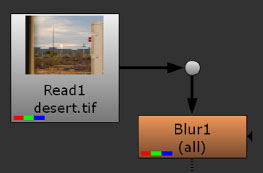
FIGURE 1.24 A right-angle pipe bend courtesy of a dot.
Exploring the Viewer Pane
Each Viewer node in the Node Graph has a Viewer panel with corresponding tab in the Viewer pane. Nuke provides Viewer1 by default, but you can create additional Viewer nodes at any time by choosing Viewer > Create New Viewer from the menu bar. Each new Viewer node is numbered consecutively. To switch between Viewer nodes, simply click the Viewer panel tabs (Figure 1.25).
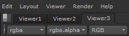
FIGURE 1.25 Three Viewer nodes indicated by three tabs in the Viewer pane.
You can connect a Viewer node to the output of any node in the Node Graph. The corresponding Viewer tab displays the output result of all the nodes upstream of the Viewer node. Any nodes downstream of the Viewer node connection are ignored. You can connect multiple Viewer nodes to multiple nodes within a single node network (Figure 1.26).
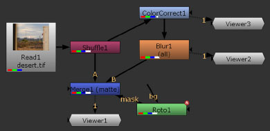
FIGURE 1.26 Three Viewer nodes connected to three different nodes in a single node network.
It’s also possible to connect a single Viewer node to multiple node outputs. To do so, LMB-drag the output pipe of a node and drop it on top of the Viewer node. Each new connection to the Viewer node is numbered consecutively. (You can also select a node and press a number key to make a new connection between the node and the Viewer1 node.) To examine the various outputs in the Viewer1 tab, press the appropriate number key while no nodes are selected. For example, in Figure 1.27, Viewer1 is connected to the output of the Blur1 node and the Merge1 node. By pressing the 1 key, the Blur1 output is displayed in the Viewer1 tab. By pressing the 2 key, the Merge1 output is displayed in the Viewer1 tab.

FIGURE 1.27 The Viewer1 node is connected to the outputs of two other nodes. When the 1 key is pressed, the output of the Blur1 node is displayed in the Viewer1 panel. In addition, the pipes involved in the display are colored orange.
Viewer panels include their own set of option buttons and cells. These are discussed throughout the book.
Resolutions, Frame Rates, and Frame Ranges
When Nuke is launched, it creates an empty project, which is known as a script. By default, the project resolution is set to 2048 × 1556, the project frames per second (fps) is set to 24, and the frame range is set to 1 to 100. You can change these settings by choosing Edit > Project Settings from the menu bar. The Project Settings panel opens in the Properties Bin pane (Figure 1.28).

FIGURE 1.28 Bottom of the Project Settings panel.
2048 × 1556, also known as full aperture, super 35, or 2K, is a resolution commonly used by the visual effects industry that matches a popular scan size for motion picture film. You can set the resolution to other commonly used sizes through the Full Size Format menu. Common video resolutions include HD (1920 × 1080 HDTV) and PC_Video (640 × 480 standard-definition TV). Resolution is measured as pixels and is written as pixel width × pixel height. In general, it’s best to set the resolution to match the resolution of the image sequences, still images, or movies you’ll import or the resolution you ultimately wish to render. Additional information on resolutions is discussed throughout this book.
You can change the project fps (or frame rate) through the Fps slider. This should be set before starting any keyframe animation. (Animation is discussed in Chapter 2.) The three most commonly used frame rates are 30 (NTSC video used in North America and Japan), 25 (PAL and SECAM video used widely outside North America), and 24 (motion picture film). Note that different flavors of HDTV support all three frame rates.
You can set the frame range, which affects the duration of the timeline, by changing the Frame Range start and end values.
You can create a new, empty script at any time by choosing File > New from the menu bar. The new script is opened in a new Nuke window.
At present, Nuke offers a limited set of options for working with interlaced video. For more detail, see Appendix B. In contrast, image sequences are progressive, whereby each frame is whole and is not broken into two interlaced fields.
Playing the Timeline
The timeline, which is included at the bottom of the Viewer pane, allows you to play back the output of a Viewer and thus show motion (Figure 1.29).
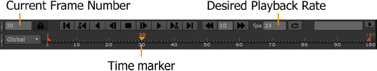
FIGURE 1.29 The timeline.
The timeline includes a standard set of playback controls. In addition, it includes the following features:
Time marker The marker is an orange upside-down triangle that you can interactively LMB-drag left or right to “scrub” through a series of frames.
Current frame number You can jump to a specific frame number by entering a value into this cell.
Desired playback speed This cell, labeled Fps, sets the desired playback rate of the timeline and is independent of the Fps cell offered by the project settings. While the timeline is playing, however, the cell reports the actual playback rate. Nuke attempts to play back in real time. For example, if Desired Playback Rate is set to 30, Nuke attempts to play exactly 30 fps. This may be impossible to achieve if the project resolution is large or the displayed node network is complex. Hence, it may be necessary to render a flipbook. The FrameCycler program, which is designed to view flipbooks, is discussed in the last section of this chapter.
Opening and Saving Nuke Scripts
Nuke scripts are saved as ASCII text files and are given the .nk extension. To open a script, choose File > Open from the menu bar. Use the File Browser window to locate the file. To save a script, choose File > Save. To save a script under a new name, choose File > Save As. To import a script into an open script, choose File > Import. If you open a script while a script is already open, the program is relaunched and you will have two iterations of Nuke running; to avoid this, first close the open script by choosing File > Close.
Nuke automatically backs up an open script every 30 seconds after the program is idle for 5 seconds. If the script has never been saved, the backup is stored in the Nuke’s Temp directory. For example, you can find the .autosave file in the C:/users/userName/AppData/Local/Temp/nuke directory on a Windows 7 system. If the script has been saved, the backup is stored in the directory where the script was previously saved. You cannot open the .autosave file through File > Open unless you rename it with an .nk extension. Otherwise, Nuke automatically retrieves the autosaved file if Nuke is launched after a program crash. You can change how often the script is backed up and where it backs up to by editing the properties in the Preferences tab of the Preferences window (Edit > Preferences from the menu bar).
Note that imported image sequences, stills, and movies are not stored within the script files. Instead, Read nodes carry an absolute path in the File field. For example, a file might be located at C:/Projects/Footage/. If the imported file is moved to a new location, Nuke will be unable to locate it. In such a situation, you must relocate the missing file by clicking the File field Browse button.
Rendering
To export a composite, you must write an image sequence or movie to disk through a Write node. (The process of writing files is often called rendering.) You can follow these steps:
1. Select the node you wish to render (do not select a Viewer node). Press the W key or RMB-click and choose Image > Write. A Write node is inserted into the network. Open the Write node’s properties panel.
2. Click the Browse button beside the File parameter. The File Browser window opens. Navigate to the directory where you want to write the files. Click the Save button. The File Browser closes and the directory path is written to the File field. Add the file name to the end of the directory path (Figure 1.30). If you are rendering an image sequence, you must add # symbols to represent the numeric placeholders. For example, you can enter test.###.ext, whereby Nuke names the files test.001.ext, test.010.ext, test.100.ext, and so on. In this case, the .ext extension represents the three-letter extension code for various file formats (.tga, .exr, and so on). If you enter a proper extension, Nuke automatically changes the File Type menu to match. (For a list of image formats and their extensions, see the “Supported Image Formats” section earlier in this chapter.)

FIGURE 1.30 Write node properties panel. A directory path and file name are entered into the File field.
3. To write out a specific frame range, select the Limit To Range radio button and enter values into the Frame Range start and end cells.
4. Once you’ve adjusted the various Write properties, launch the render by clicking the Render button.
If you prefer to render a QuickTime or AVI movie, set the File Type menu to FFmpeg and add a .mov or .avi extension to the file name. For more information on the FFmpeg library, see the “Supported Image Formats” section earlier in this chapter.
Playing Back with FrameCycler
Although the playback controls provided by the timeline are convenient, their features are somewhat limited. In addition, playing back through the timeline does not necessarily guarantee that the sequence will achieve real-time speed. As a solution, Nuke offers FrameCycler, which is an advanced playback program that comes bundled with the software. To play back with FrameCycler, however, you must create a flipbook, which is a specially prepared, prerendered sequence of frames. To create a flipbook, follow these steps:
1. Select a node you wish to flipbook. It’s not necessary to select a Write node. You can select any node in a network. Choose Render > Flipbook Selected from the menu bar or press Opt/Alt+F. The Flipbook dialog box opens. Enter a frame range into the Frame or Frame Range cell. For example, enter 1–30 to render frames 1 to 30. Press the OK button.
2. The flipbook renders. A Progress dialog box displays its namesake. When the render is finished, the FrameCycler window opens. The flipbook is loaded onto the timeline and is ready for playback.

FIGURE 1.31 The FrameCycler window.
3. The FrameCycler offers a standard set of playback controls (Figure 1.31). The first time the program plays the flipbook, it’s loaded into memory. Subsequent playbacks attempt to achieve real-time speeds.
4. To zoom in or out, change the Resample menu from Resample Off to a percentage such as 50%. To reposition the flipbook within the player, MMB-drag.
You can use the FrameCycler to review an image sequence or movie that is already written to disk. To do so, follow these steps:
1. You cannot launch the version of FrameCycler that’s bundled with Nuke outside Nuke. Therefore, if FrameCycler is not already running, you must go through the Nuke’s flipbook feature. To avoid wasting time on a complete flipbook render, you can select a random node, press Opt/Alt+F, and enter 0 into the Frames To Flipbook Frames cell. The first frame of the sequence is rendered as a one-frame-long flipbook. To delete the flipbook, click the X button at the top left of the FrameCycler timeline.
2. Once the FrameCycler window is open, click the Desktop button at the bottom left. (If you don’t see the button, maximize the window.) The file browser opens. To display the directory tree, click the Tree button at the top left. Navigate to an image sequence or movie and double-click its icon. The sequence is placed on a new timeline. To return to the viewer, click the Desktop button once again. The sequence is ready to play back.
FrameCycler is a complex program with numerous options that are beyond the scope of this book. For additional documentation, see the FrameCycler_Pro_User_Guide PDF in the NukeProgramDirectory/FrameCycler Windows/doc/ directory on the DVD.
Part 1: Setting Up a New Script
Tutorial 1 carries you through the steps needed to add a rendered 3D still image to live-action video footage. Part 1 of the tutorial sets up a new script, imports the necessary files, adjusts the resolution through the addition of a Reformat node, and creates a simple composite through a Merge node.
1. Launch Nuke. Click the Image icon on the toolbar and choose Read from the dropdown menu. Alternatively, you can place the mouse in the Node Graph, RMB-click, and choose Image > Read from the shortcut menu. A new node, Read1, is placed in the Node Graph. Simultaneously, the File Browser window opens. Navigate to the Tutorials/Tutorial1/Plates/kick/ directory. (See the Introduction for tips on working with files on the DVD.) Click on the kick.##.tga 0 59 image sequence name (this may also appear as kick.%02d.tga 0 59). Click the Open button. The File Browser window closes and the image sequence is loaded into the Read1 node.
2. Note that the bounding box is set to a default resolution of 2048 × 1556, which is provided by the 2k_Super_35(full ap) resolution preset. To view the imported sequence, connect the Viewer1 node to the Read1 node. To do this, LMB-drag the dotted Viewer1 input pipe and drop it on top of the Read1 node. Alternatively, you can click the Read1 node so that it becomes selected (selected nodes turn a pale orange) and press the 1 key on the keyboard. As soon as Viewer1 is connected, the sequence is visible in the Viewer1 panel and the bounding box is reset to 1280 × 720, which is the resolution of the sequence (Figure 1.32). The sequence features a character reaching for an unseen object, which in turn is kicked away by a second character.

FIGURE 1.32 Kick sequence, as seen in the Viewer1 panel with the current frame set to 58. The resolution of the sequence is 1280 × 720.
3. Choose Edit > Project Settings from the menu bar. In the Project Settings panel, change the Fps parameter to 30. The image sequence was derived from a video shot at 30 fps. To ensure that the characters move at their original speed, the fps must be matched between the video and the project. Change the frame range to 0, 59. The image sequence is 60 frames long.
4. Create a new Read node. In the File Browser window, navigate to the Tutorials/Tutorial1/Renders/heart/ directory. Click on the heart.exr file name and click the Open button. Disconnect the Viewer1 node from the Read1 node and connect it to the Read2 node. The new sequence features a still 3D render of a stylized heart. Black surrounds the heart, which indicates empty 3D space (Figure 1.33). You can check the render’s alpha channel by placing the mouse in the Viewer panel and pressing the A key. White indicates opaque pixels, black indicates transparent pixels, and gray indicates semi-transparent pixels. Hence, when viewing the render’s alpha channel, the heart appears white (Figure 1.34). To return to the RGB view, press the A key again. You can also switch between channels by changing the Display Style menu at the top of the Viewer pane; the menu is set to RGB by default, but may be changed to A for alpha. (Alpha channels are discussed in more detail in Chapter 4.) Note that the Read node’s Colorspace menu is set to Linear by default. This prevents the node from converting the render with a color space look-up table (LUT). In this case, the Linear setting prevents the heart from taking on unnecessary contrast. Color spaces and LUTs are discussed in Chapter 3.

FIGURE 1.33 Heart render, as seen in the Viewer1 panel. The resolution of the sequence is 2048 × 1556. (Heart modeled by Gerardo Perusquia Montes.)
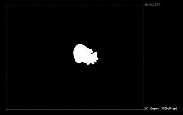
FIGURE 1.34 Alpha channel of same render.
5. The resolution of the heart render is 2048 × 1556. The resolution mismatch between the kick sequence and the heart render will lead to problems unless addressed. There are two solutions in this situation: You can scale up the kick sequence or scale down the heart render. Assuming that a resolution of 1280 × 720 is sufficient for the final render, you will maintain better quality if you scale down the heart render. Scaling up requires the synthesis of new pixels, which leads to a softening of the image. (For more information on scaling, see Chapter 2.) To scale down the heart render, you can use a Reformat node. Select the Read2 node, RMB-click, and choose Transform > Reformat from the shortcut menu. In the Reformat1 node’s properties panel, change the Output Format menu to 1280 × 720. The output is instantly scaled.
6. Because the render includes an alpha channel that stores transparency information, you can place the heart “on top” of the image sequence by creating a Merge node. To do so, press the M key or RMB-click in the Node Graph and choose Merge > Merge from the shortcut menu. A Merge1 node is added to the Node Graph. Connect the input B pipe of the Merge1 node to the output of the Read1 node. The input B pipe is designed to accept a background image or what might be considered the “lowest layer” or a layered composite. Connect the input A pipe to the output of the Reformat1 node. Connect the Viewer1 input pipe to the output of the Merge1 node. (See Figure 1.36 for the final node network layout.) The heart is composited on top of the video footage (Figure 1.35). For more information on node connection, see the “Connecting, Disconnecting, and Branching Pipes” section earlier in this chapter. Merge nodes are discussed in more detail in Chapter 4.
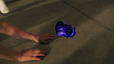
FIGURE 1.35 The heart is composited on top of the image sequence through the use of a Merge node.
This concludes Part 1 of Tutorial 1. Choose File > Save As to save a copy of the script. A sample Nuke script is included as Tutorial1.1.nk in the Tutorials/Tutorial1/Scripts/ directory on the DVD. In Chapter 2, we’ll continue to refine the composite by keyframe animating the transformations of the heart render. As an extra step, you can spend time refining the current node network layout. For example, you can add dots to create right-angle bends in the pipes and/or add backdrops to define particular areas of the network. For example, in Figure 1.36 a dot is added to the pipe running between the Read1 node and the Merge1 node. You can add a dot by selecting the Read1 node, RMB-clicking, and choosing Other > Dot from the shortcut menu. To add a backdrop, Shift-click the Read2 node and Reformat1 node, RMB-click, and choose Other > Backdrop from the shortcut menu. For more information on dots and backdrops, see the “Organizing the Node Graph” section earlier in this chapter.

FIGURE 1.36 The final node network for Part 1 of Tutorial 1. A dot and backdrop are added for additional network clarity.