|
|
|
|
Optimization, Scripting, and New Techniques |
|

It’s important to organize and optimize every Nuke script, whether it’s simple or complex. The program provides various ways to group nodes, reduce calculation and rendering times, and automate common functions. The creation of links, expressions, and scripts can take the organization and automation even further by allowing you to create nodes, node connections, math-driven parameters, and custom interface elements through programming commands and saved script files.
This chapter includes the following critical information:
• Script optimization
• Gizmos and Group nodes
• Basics of TCL and Python scripting
• Links and expressions
• Deep compositing and particles
Organizing and Optimizing a Script
If you construct a large node network, the Node Graph can become difficult to navigate and interpret. In addition, if you work with large-resolution image formats or apply various processor-intensive filter nodes, Nuke may slow significantly as it calculates each frame. Thus, it is often necessary to organize and optimize the script. Nuke provides means to set program preferences, work with proxy resolutions, precomp outputs, create Group nodes and exportable gizmos, and annotate the network with notes.
System Preferences
Nuke provides a long list of user-defined preferences. These are accessible by choosing Edit > Preferences from the menu bar. The Preferences window includes the following tabbed sections:
• Preferences includes autosave, disk cache, and memory usage settings.
• Windows controls the functionality of GUI elements such as tooltips and snapping.
• Control Panels determines the behavior of the Properties panel.
• Appearance sets the program font and component colors.
• Node Colors sets its namesake. Note that the colors are divided into various categories, such as Drawing, Merge, or Keyer, and specific node names are typed in each category cell.
• Node Graph establishes the graphic qualities of pipes, arrows, and node boxes.
• Viewer sets the interactive qualities of the Viewer tabs. If you are working in Nuke’s 3D environment and wish to mimic the camera controls of another program (e.g., Maya), change the 3D Control Type menu.
• Script Editor controls the font and colors used in the script field.
Customizing the Interface
You can customize the pane, panel, and tab layout of Nuke in several ways:
• You can close any tab (Node Graph, Curve Editor, Properties Bin, Script Editor, Group Node Graph, and so on) by RMB-clicking over the tab name and choosing Close Tab. Conversely, you can open any tab in any pane by LMB-clicking over the pane’s Content Menu button (at the top left of the pane, as seen in Figure 10.1) and choosing the name of the tab from the dropdown menu (e.g., choose Node Graph).
• You can subdivide a pane into two panes by LMB-clicking the pane’s Content Menu button and choosing Split Vertical or Split Horizontal. You can close a pane by choosing Close Pane for the Content Menu. You can break a pane or tab away from the main window and “float” it by choosing Float Pane or Float Tab from the Content Menu.

FIGURE 10.1 The Content Menu button, as seen to the left of a Node Graph tab.
• You can save a current pane layout by choosing Layout > Save Layout n from the menu bar. You can restore a saved pane layout by choosing Layout > Restore Layout n.
Proxy Formats, Downrez, and Viewer Refresh
By default, Nuke processes the node network at full resolution, as determined by the Full Size Format parameter of the Project Settings properties panel. However, you can use a proxy resolution to temporarily speed up the node network processing. To do so, choose Edit > Project Settings, select the Proxy Mode checkbox, and set the Proxy Mode menu to Scale or Format (Figure 10.2).
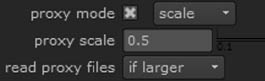
FIGURE 10.2 The Proxy section of the Project Settings properties panel.
Scale forces the composition to be scaled to a percentage set by the Proxy Scale slider. For example, if Proxy Scale is set to 0.5, the composition becomes 50% of the resolution size. The resulting pixel size is indicted by the output bounding box in the Viewer. The Format option scales the composition to a standard resolution, as is indicated by the Proxy Format menu. The Read Proxy Files menu determines how imported bitmaps, image sequence, and movies are interpreted by a Read node when the Proxy mode is activated. Regardless of the Read Proxy Files menu setting, the final output of the node network remains the proxy resolution. To return the composition to the full project resolution, deselect the Proxy Mode checkbox. You can remotely toggle on and off the Proxy Mode checkbox by pressing Cmd/Ctrl+Por clicking the Toggle Proxy Mode button at the top right of the Viewer tab (Figure 10.3).
FIGURE 10.3 Left to right: Toggle Proxy Mode button, Downrez menu, Region-of-Interest button, Recalculate button, and Pause button.
In addition to choosing a proxy format, you can downrez (downscale) the current Viewer input by choosing a non-one value from the Downrez menu (see Figure 10.3). For example, if you set Downrez to 4, the input is scaled to one-fourth its original resolution.
You can prevent the Viewer from updating the entire bounding box by clicking the Region-of-Interest button (see Figure 10.3) so that it turns red. A region-of-interest handle appears in the Viewer. You can interactively LMB-drag the handle center to transform it or LMB-drag the handle corners to rescale it. If the node network is altered, only the area within the region-of-interest is updated. Additionally, you can force the Viewer to update by clicking the Recalculate button or pause a slow update by clicking the Pause button (see Figure 10.3).
Precomping and Caching
The Nuke Precomp node (Other > Precomp) acts as a subroutine, whereby a portion of a node network is exported as a separate Nuke script. The Nuke script is then re-read by the Precomp node and presented to the master script as a single output. This allows multiple artists to work on separate portions of a master script. To apply the Precomp node, follow these steps:
1. Select a node that has an upstream network you’d like to capture. RMB-click over the node and choose Other > Precomp. The Precomp Nodes dialog box opens (Figure 10.4). The Precomp script name and path are listed as well as the precomp render name, path, and file format (indicated by the file extension). You can change names and paths or leave them intact. Press the OK button. A new Precomp node is created. The Precomp node’s output is connected to the network downstream of the node originally selected (Figures 10.5 and 10.6). By default, the original nodes are assigned to a new Background.
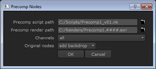
FIGURE 10.4 The Precomp Nodes dialog box.
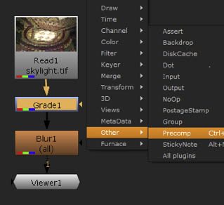
FIGURE 10.5 A Grade node is selected and Other > Precomp chosen.
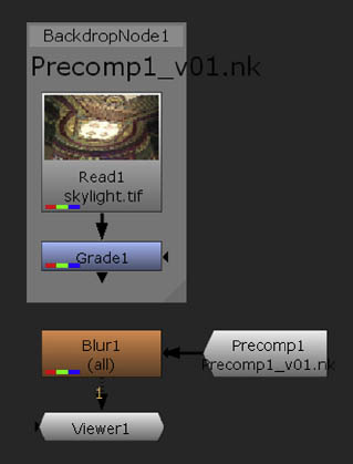
FIGURE 10.6 The resulting Precomp node’s output is connected to the Blur node, while the Grade and Read nodes are separated and indicated by a new Background.
2. Open the Precomp node’s properties panel. The precomp script is listed. You can force the node to render an image sequence and thus save calculation time by clicking the Render button. When the Render is complete, the Read File For Output checkbox is automatically selected and the rendered files are used for the node’s output. The node icon turns green to indicate this. You can force the node to use the saved script instead of the renders by deselecting the Read File For Output checkbox.
In contrast, the DiskCache node, in the Other menu, writes the scanline data produced by the upstream node network to a temporary disk cache. (Scanlines are rows of pixels sent to the Viewer.) This allows downstream nodes to use the disk cache data and thus skip the necessity of calculating the upstream scanlines until the upstream network is changed. The cache location is set by the Preferences window (Edit > Preferences from the menu bar).
Splitting the Viewer
A Viewer node can accept 10 inputs. Each input is consecutively numbered. You can quickly connect an input to a Viewer by selecting the input node and pressing a number key, such as 2, 3, or 4. If two or more inputs exist, you can toggle between them by pressing the 1 through 9 keys on the keyboard (pressing 0 switches to input 10). Once two or more inputs exist, you can create a split screen with one input on the left and another input on the right. To activate the split, change the Composite menu, at the top center of the Viewer panel, to Wipe (Figure 10.7). Change the Read A menu to one input. Change the Read B menu to a second input.
FIGURE 10.7 Left to right: Read A input menu, Composite menu, and Read B input menu.
A wipe handle is placed at the center of the bounding box (Figure 10.8). You can LMB-drag the handle left or right to change the split line. You can reduce the opacity of the Read B input by LMB-dragging the diagonal line at the top right of the handle. For example, in Figure 10.8, Viewer1 carries two inputs. The first input is provided by a Read node and the second input is provided by a Blur node that blurs the Read node’s bitmap.
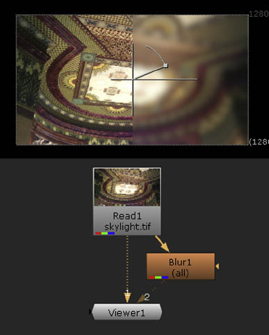
FIGURE 10.8 A wipe handle, provided by the Wipe setting of the Composite menu, combines two inputs. In this case, input A is set to the Viewer input 1, which is the unaltered Read1 node. Input B is set to the Viewer input 2, which is the Blur1 node.
Using Metadata
You can loosely define metadata as data about data. In the realm of digital photography and cinematography, metadata is hidden information carried by a file. For example, a bitmap created by a digital still camera can carry metadata in an EXIF (exchangeable image file format) where the photo’s date of creation, the camera’s f-stop, file bit depth, file size, and similar information is stored. In Nuke, you can view or modify existing metadata. You can also create custom metadata to fit the specific project you are working on. Nuke provides the following metadata nodes through the MetaData menu.

FIGURE 10.9 A small portion of the metadata carried by a bitmap. A ViewMetaData node is connected to the output of a Read node.
ViewMetaData displays metadata flowing into its input pipe (Figure 10.9).
ModifyMetaData allows you to overwrite existing metadata. You can modify the data one key at a time. A key is a variable with a specific name and value. For example, a key name may be Exif/FocalLength and the key value may be 35. To modify a key, click the + button, double-click the orange cell below the Key column, select a key name in the Pick Metadata Key dialog box, double-click the orange cell below the Value column, and type the new value into the cell. You can add a custom key by typing a key name into the Pick Metadata Key dialog box text cell.
AddTimeCode adds time code (HH:MM:SS) to the metadata stream as a new key. The key is listed as Input/timecode.
CopyMetaData allows you to copy metadata from a node connected to the Meta input pipe. You can copy all the keys and values or choose a specific key name.
CompareMetaData compares metadata between its input A and input B pipes. Differences with key names and key values are listed in the node’s properties panel.
Sticky Notes and Postage Stamps
Nuke provides the StickyNote node, which you can use to annotate a node network. The StickyNote text appears in the Node Graph, but is not connectable to other nodes. The PostageStamp node, on the other hand, creates a node-sized thumbnail of its input. The PostageStamp node allows you to check a portion of a network without having to reconnect or create a Viewer node. Both nodes are available through the Other menu.
Creating Groups
Nuke node networks often become complex and difficult to interpret. Thus, Nuke provides a means to group nodes together. When nodes are grouped, they are replaced by a Group node and are otherwise hidden in the Node Graph. However, the nodes are accessible through their own Group tab. To create and utilize a Group node, follow these steps:
1. Shift+select the nodes that you would like to convert to a group. Choose Other > Group. A new Group node replaces the selected nodes in the Node Graph. In addition, the original nodes appear in a new Group tab named Groupn Node Graph (Figure 10.10).
2. You can manipulate the original nodes within the Group tab. This includes changing parameter values, animating parameters, deleting nodes, adding nodes, and connecting or disconnecting pipes. That said, do not change the new Input or Output nodes as they represent incoming and outgoing connections to the Group node.
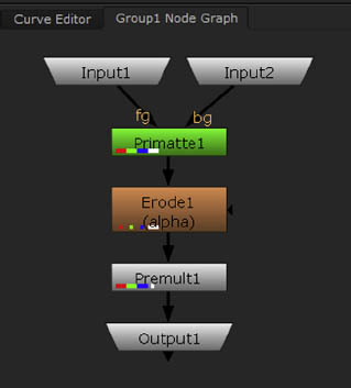
FIGURE 10.10 The contents of a Group node, as seen in the Group node’s Node Graph tab.
3. To close the Group tab, RMB-click over the tab name and choose Close Tab from the dropdown menu. To open the Group tab of a Group node, select the Group node and choose Edit > Node > Group > Open Group Node Graph from the menu bar or press Cmd/Ctrl+Enter.
4. To delete a Group node and restore the original nodes to the Node Graph, select the Group node and choose Edit > Node > Group > Expand Group from the menu bar.
Writing and Reading Gizmos
In Nuke, a gizmo is a set of nodes or a node network that is saved as a unique script. Gizmos are useful sharing sections of larger scripts among multiple compositors or savings routines that are used in multiple scripts over the duration of a lengthy production. To create and read a gizmo, follow these steps:
1. Select a Group node. (To create a Group node, see the prior section.) Open the Group node’s properties panel. Click the Export To Gizmo button. In the file browser, choose a name and location to write the gizmo file to. Gizmo files are special text files that carry the .gizmo extension.
2. To read a gizmo file, choose File > Import Script from the menu bar. A new, unconnected Gizmo node is placed in the Node Graph. Although a Gizmo node represents a set of nodes with specific connections and parameters settings, the nodes are not visible. To access the original nodes, choose Edit > Node > Group > Expand Group from the menu bar.
Managing Knobs
In Nuke, a knob is a specific parameter of a specific node. In general, a knob is represented by a slider, numeric cell, or checkbox. You can add a custom knob to a node at any time. This may be useful for creating custom parameters when scripting with Python or TCL. To add a knob, follow these steps:
1. RMB-click over an empty area of a node’s properties panel and choose Manage User Knobs from the dropdown menu. An unlabeled knob dialog box opens. Click the Add button and choose a parameter style from the dropdown menu. For example, select Integer Knob to create a numeric cell.
2. A new knob dialog box opens (Figure 10.11). Enter a parameter name into the Name field (this is the variable name used by expressions and similar scripting). Enter a name into the Label field (a label is the name that appears to the left of the parameter slider, cell, or checkbox). Optionally, enter text into the Tooltip field (a tooltip is the descriptive text that appears when the mouse hovers over the parameter). Click the OK button. The box closes and the new knob is added to the user knob list. Click the Done button of the unlabeled dialog window. The new knob is added to the User tab of the node’s properties panel.
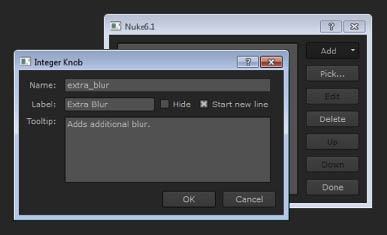
FIGURE 10.11 Knob dialog boxes. The top box sets the name, label, and tooltip for the added knob.
3. Additionally, you can add a standard Nuke knob by clicking the Pick button instead of the Add button and selecting the knob name from the Pick Knobs To Add dialog box. To delete a user knob, RMB-click over an empty area of a node’s properties panel, choose Manage User Knobs, highlight the knob name in the unlabeled knob dialog box, and click the Delete button.
For more information on Python and TCL scripting, see the following “Scripting and Expressions” section.
Updating Help Boxes
When you click the question mark at the top right of a node’s properties panel, a default help message appears in a yellow dialog box. You can change the help message by RMB-clicking over an empty area of the properties panel and choosing Edit Help from the dropdown menu. A Edit [?] Help Message dialog box opens, which you can type into. Note that any change affects the current node but no other node (old or new) is affected.
Scripting and Expressions
Scripting is a form of programming that provides greater control over a program such as Nuke. Nuke supports TCL and Python scripting through the Nuke interface. In addition, Nuke provides a means to create expressions. Expressions are small mathematical formulas with which you can automatically update parameter values.
Introduction to TCL
Nuke is built on the Tool Command Language (TCL), which is an open-source programming language. You can use TCL commands to manipulate the timeline, customize the Nuke interface, expand the functionality of nodes, retrieve node information, and read or write to or from Nuke scripts and other databases.
To enter a TCL command, choose File > Script Command from the menu bar or press the X key in the Node Graph to open the Script Command dialog box (Figure 10.12). Select the TCL radio button and enter the command in the Command field. Click the OK button to execute the command.
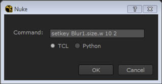
FIGURE 10.12 Script Command dialog box.
A few TCL commands are included here. Note that the term knob is often used by Nuke to refer to a specific node parameter.
• version returns the current version of Nuke in a dialog box.
• memory info prints a detailed memory report, including node memory demands, convolution filter sizes, and resolutions passed between nodes to Viewers.
• frame n moves you to frame n on the timeline.
• setkey knob n value sets a keyframe for the named knob on frame n with a stated value. The proper knob name must be used and should include the node name, parameter name, and channel name separated by periods. For example, a proper knob name is Blur1.size.w. Thus, a command might be setkey Blur1.size.w 10 2.
• knobs -a node lists all the knobs carried by a node in a dialog box. Commonly used knobs represented by cells, sliders, and checkboxes appear first in the list.
• script_save_as name saves the script. For example, enter script_save_as C:/comp/test.nk.
• menu "menu_name""hotkey""icon_name""tooltip"{command} adds a custom menu to the menu bar. When the menu is selected, a TCL command is executed. For example, to create a custom undo menu that uses the F1 hotkey, enter menu "Undo" "F1" "" "" {undo}. Empty quotes signify that a particular option is not used, such as an icon bitmap name and tooltip text. Note that the custom menu is not permanent and disappears if Nuke is restarted.
You can also execute a TCL command in the Script Editor. However, you must precede the command with a Python command nuke.tcl and place the TCL command within parenthesis and quotes. For example, enter nuke.tcl ("memory info"). For information on the Script Editor and the Python scripting language, see the next section. For a detailed list of TCL commands, choose Help > Documentation and click on the TCL Scripting link in the browser that opens.
Introduction to Python
Python is an open-source, dynamic scripting language used widely in the realm of 3D animation and digital compositing. Nuke supports the use of Python scripting through its Script Editor. You can open the Script Editor by clicking a Content Menu button at the top-left corner of a pane and choosing Script Editor from the menu. The Script Editor appears in a new tab, which you can close at any time by RMB-clicking the tab name and choosing Close Tab.
The Script Editor is divided into two sections: a top Output window and a bottom Input window. You can type a Python script in the Input window and execute the script by pressing Cmd/Ctrl+Enter. For example, type print "Nuke Rocks" and press Cmd/Ctrl+Enter. The Input window is cleared and the result of the script is displayed in the Output window (Figure 10.13).
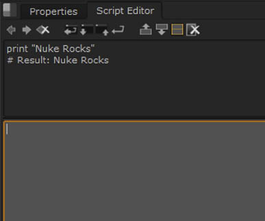
FIGURE 10.13 Top-left corner of the Script Editor tab. The Input window is light gray and the Output window is dark gray.
Python Object.Method Examples
Python is an object-oriented language. An object is a unique data set. Similar objects are considered instances of a class. Classes are grouped together into modules. Objects within a class provide various means to manipulate the contained data, each of which is known as a method. Within Nuke, a Python command is composed of an object and a method separated by a period. As such, the syntax follows object.method(value), where value is a variable passed to the method to alter its behavior. For example, the command nuke.message(“Nuke Rocks”) creates a dialog box with the text “Nuke Rocks”; in this case, nuke is the object and message is the method.
Nuke provides a long list of modules, classes, objects, and methods. For a detailed description of these components, choose Help > Documentation and click on the Python Scripting link in the browser that opens. A few example object.method commands follow (note that Python is sensitive to capitalization):
• nuke.undo() undoes the previous step.
• nuke.frame(n) moves to frame n on the timeline.
• nuke.selectAll() selects all the nodes in the Node Graph.
• nuke.createNode(“node_name”) creates a new node. A standard node name, such as Blur, must be entered within the parentheses.
• nuke.addFormat(“width height pixel-aspect-ratio format_name”) adds a new format to the Project Settings panel Full Size Format menu. For example, enter nuke.addFormat(“1280 720 1 720HD”) to create an HDTV format.
• nuke.value(“knob”) returns the value of a knob. The knob name must include the node name, parameter name, and channel name. For example, enter nuke.value(“Blur1.size.w”) to retrieve the current value of the Size parameter of the Blur1 node.
• nuke.extractSelected() breaks connections between selected nodes and the rest of the network and moves the selected nodes to the right.
• nukescripts.autoBackdrop() adds a backdrop to a selected node.
• nukescripts.infoviewer() prints the state of a selected node in a dialog box, including the current value of every knob.
Note that you can enter Python commands into the Script Command dialog box. Press X in the Node Graph and select the Python radio button.
Python Variables and Operators
Python scripting supports the use of variables. A variable is a value that may change within the scope of a program or script. You can create a variable by choosing a variable name and declaring what it’s equal to. For example, Cmd/Ctrl+Entering val=10 creates the variable val and declares that it is equal to 10. You can retrieve the variable value at a later time. For example, Cmd/Ctrl+Entering print val displays 10 in the Output window. There are three common variable types, each of which you must declare differently:
|
integer |
|
float |
|
string |
In addition, you can assign nodes to variables. This allows you to retrieve or update the node’s parameter values at a later time. The following are example commands:
• bn=nuke.createNode(“Blur”) creates a new Blur node and assigns it to the bn variable.
• bn["size"].getValue() displays the Blur node’s Size parameter value.
• newvar=bn["size"].getValue() assigns the parameter value to a new variable, newvar.
• bn["size"].setValue(10) updates the Size parameter value to 10.
You can update a variable value at any time. In addition, you can apply mathematical operators. For example, you can Cmd/Ctrl+Enter the following:
val=0
val=val+100
print val
To enter a multiline script, press the Enter key at the end of each line and press Cmd/Ctrl+Enter to execute the script. Python uses the following mathematical symbols: + (plus), × (minus), * (multiply), and / (divide). In fact, you can use the print command as a calculator; for example, print 2048*.13 displays 266.24 in the Output window.
Python supports complex programming structures such as if statements and for loops. For example, the following script locates every Blur node in the script and tests whether its input is connected to a Read node. If the Read node is present, the Size value is changed to 5.
for nodename in nuke.allNodes():
     if nodename.Class() == "Blur":
          if nodename.input(0).Class() == "Read":
               nodename["size"].setValue(5)
In this case, the double equals sign (==) is required when comparing variables with an if statement. The for statement cycles through all the Nuke nodes found within the Node Graph; with each step, the variable nodename is set to one node. The first if statement tests whether or not the nodename variable is a Blur node. If the first if statement is true, the second if statement tests whether the Blur node’s input pipe is connected to a Read node. If the second if statement is true, the Blur node’s Size parameter is set to 5. If either of the if statements are false, the script jumps back to the first line. Note that Nuke is sensitive to indentation when for and if statements are involved. For more information on Python syntax and programming structures, visit www.python.org.
Managing Hotkeys
Nuke provides an extensive list of hotkeys for various nodes and operations. To examine the list, choose Help > Key Assignments from the menu bar. To edit the hotkey assignments, you must update the menu.py Python file. By default, the file is placed in the Nuke plug-ins directory. For example, on a Windows 7 64-bit operating system, the file is located at the C:Program FilesNuke[version_number]plugins directory. If you are running a non-Windows system, you can use the Python command nuke.pluginPath() to find the directory. Within menu.py, each Nuke menu item and associated hotkey is declared. For example, the following two lines create the File menu and Save submenu in the menu bar:
m = menubar.addMenu(“&File”)
m.addCommand(“&Save”, “nuke.scriptSave(””)”, ”^s”)
In this case nuke.scriptSave is the object.method Python command associated with the Save menu and ^s represents the Cmd/Ctrl+S hotkey. You can alter the hotkeys by using such symbols as ^ for Cmd/Ctrl, ^# for Cmd/Ctrl+Opt/Alt, and + for Shift. Once you save the menu.py file in a text format and restart Nuke, the hotkey updates take effect. You can also edit the menu.py script to add or remove your own custom menus. For example, to add your own menu named “Quit” to the menu bar with a submenu that closes the Nuke script with a Cmd/Ctrl+Q hotkey, add the following lines:
m = menubar.addMenu(”&Quit”)m.addCommand(“&Quit Script”, “nuke.scriptClose()”, “^q”)
Script Editor Buttons
The Script Editor includes a row of buttons that allow you to open and save Python scripts, cycle through script history, and control the Input and Output windows. These are illustrated by Figure 10.14 and are described here.
Previous Script/Next Script loads previously executed scripts. The scripts appear in the Input field.
Clear History clears the script history used by Previous Script/Next Script.
Source A Script loads a script into the program and executes it immediately. The result of the script is displayed by the Output window.
Load A Script loads the script into the Input window but does not execute it.
Save A Script saves the Input window script as a text file with the .py extension. You can edit a .py file with an external text editor, such as Windows Wordpad.
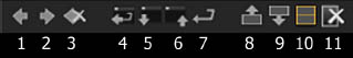
FIGURE 10.14 Script Editor Buttons: (1) Previous Script, (2) Next Script, (3) Clear History, (4) Source A Script, (5) Load A Script, (6) Save A Script, (7) Run The Current Script, (8) Show Input Only, (9) Show Output Only, (10) Show Both Input And Output, and (11) Clear Output Window.
Run The Current Script runs the Input window script. It has the same functionality as Cmd/Ctrl+Enter.
Show Input Only/Show Output Only determine if Input and/or Output windows are visible.
Clear Output Window fulfills its namesake.
Working with Links and Expressions
In Nuke, you can link two parameters together, forcing the second parameter to adopt the values of the first parameter. After a link is created, the relationship between the parameters is automatically maintained until the link is removed. To create a link, follow these steps:
1. Open the properties panels for the two nodes you wish to connect with a link. Determine which node will be the “parent” and which will be the “child” (the parent supplies values to the child). Determine which parameters are to be linked.
2. Cmd/Ctrl+LMB-drag from the parent parameter Animation Menu button to the child parameter Animation Menu button. For example, Cmd/Ctrl+LMB-drag from the Rotate Animation Menu button of one node to the Rotate Animation Menu button of a second node. A green link line is drawn between the nodes in the Node Graph. An arrow indicates the flow of information (Figure 10.15).
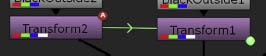
FIGURE 10.15 A link drawn between two nodes.
3. Test the link by updating the parameter value of the parent node. The child node parameter value changes automatically. The link will remain until you LMB-click the child node’s Animation Menu button and choose No Animation.
A link represents a simple expression. Initially, the expression carries a 1-to-1 relationship, where the child value is exactly equal to the parent value. You can modify the expression, however, by LMB-clicking the child Animation Menu button and choosing Edit Expression. The Edit Expression dialog box opens and displays the initial expression (Figure 10.16).
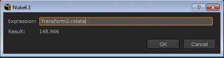
FIGURE 10.16 Expression dialog box.
The expression uses the syntax node.parameter.channel where node is the node name, parameter is the parameter name, and channel is the optional channel name, such as x, y, z, w, h, and so on. (Nuke may add the word parent to the start of the expression; the expression will function with or without it.) You can update the expression by adding a mathematical formula. For example, to reduce the rotation of the child parameter to half of the parent parameter, add /2 to the end of the expression line. To update the expression click the OK button. For example, in Figure 10.17 the Rotate parameters of two Transform nodes are linked. The child parameter, which affects a yellow Constant square, rotates four times faster than the parent parameter, which affects a smaller red Constant square. The expression is written as Transform2.rotate*4.
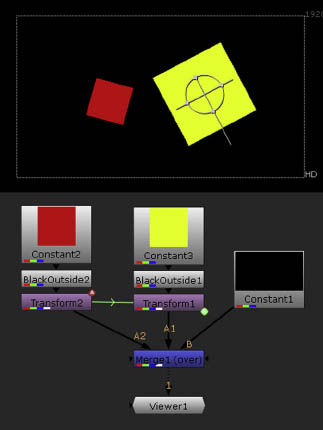
FIGURE 10.17 A link causes a yellow Constant to rotate four times faster than the red Constant. The red Constant’s Transform node is animated, while the yellow Constant carries no animation. A sample script is included as linking.nk in the Chapters/Chapter10/Scripts/ directory on the DVD.
Much like the CornerPin2D node (see Chapter 8) the Stabilize2D node requires expressions to work. The general work flow for the Stabilize2D node follows:
1. Create motion paths for an input using a Tracker node (see Chapter 8). Two tracks are often necessary, so activate Tracker1 and Tracker2.
2. With the Tracker node selected, choose Transform > Stabilize. Change the new Stabilize2D node’s Type menu to 2 Point.
3. Enter 1—into the Stabilze2D node’s Track1 X and Y and Track2 X and Y cells. This inverts the incoming motion path data.
4. Create links or expressions between the Tracker node’s Tracker1 and the Stabilize2D node’s Track1 parameters. (The Tracker node is the parent and the Stabilize2D node is the child.) Do the same for Tracker2 and Track2. For example, the final expression for Track1 X should look like 1—Tracker1. tracker1.x.
5. Adjust the Stabilize2D node’s Offset X and Y parameters to slide the output back into the output bounding box area.
As an alternative to Cmd/Ctrl+LMB-dragging between Animation Menu buttons, you can LMB-click a child Animation Menu button and choose Add Expression. The Expression dialog box opens. If the parameter carries more than one channel, each channel receives its own expression field. In this situation, there is no initial expression and you must type one from scratch. Note that you can “mix and match” parameters when creating expressions. For example, you can link Rotate to Translate X. In such a case, you can Cmd/Ctrl+LMB-drag between the Rotate Animation Menu button and the Translate X numeric cell.
Using Expression and Math Nodes
The Expression node, available through the Color > Math menu, allows you to affect color, alpha, depth, and motion channels with complex expressions. The node’s properties panel offers four Channels menus, which you can set to the channel or channels of your choice (Figure 10.18). Below each channels menu is an = field, into which you can type an expression. For example, to set the input alpha channel to 1, set the first Channels menu to Alpha and enter 1 into the first = field.
To make the expressions more complex, you can add mathematical operators or functions. Functions signify a complex value or math operation with a simple name. For example, to assign each pixel of the green channel with a random value plus 0.2, set one of the Channels menus to RGB, select the matching Green checkbox, and enter random + 0.2 into the matching = field (Figures 10.19 and 10.20).
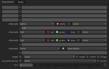
FIGURE 10.18 The Expression node properties panel. The first Channels menu selects the alpha channel, which in turn is set to a value of 1 by the first = field.
To see a full list of functions supported by Nuke, choose Help > Documentation and click the Knob Math Expressions link in the browser that opens. Other useful functions include pi (value of pi, rounded off to 3.141592654), sqrt(x) (square root of x), log(x) (natural logarithm of x), and pow(x, y) (x raised to the power of y). If a function requires a variable, like x or y, you can use a fixed value or a channel name. For example pow(red, 2) is equal to the red channel pixel value to the power of 2. Note that the Expression dialog box, described in the previous section, supports the use of functions.
FIGURE 10.19 Each pixel of the green channel is brightened by adding 0.2 and a random value assigned by the random function.
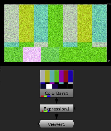
FIGURE 10.20 The result of the expression on a ColorBars node. A sample script is included as expression.nk in the Chapters/Chapter10/Scripts/ directory on the DVD.
At the top of the Expression node’s properties panel, four slots are provided for creating temporary variables. For example, if you enter t = pow(r, g), then the variable t is equal to the red channel pixel value to the power of the green channel pixel value. Once a variable is established, you can use it in any of the = fields below the Channels menu.
The remaining nodes in the Color > Math menu apply mathematical operations to their input. The Add node adds a value set by the Value parameter to every pixel within the channels defined by the Channels menu. The Multiply node multiplies the value. Gamma applies a power function. The ClipTest node adds a zebra-stripe pattern to any part of the input that exceeds the values set by the Lower and Upper parameters. ColorMatrix multiplies the input by a 3 − 3 matrix, which is useful for converting one color space to another.
New Techniques
Nuke v6.3 adds several new techniques: deep compositing, image-based modeling, and in-program particle generation. These techniques are explored in this section.
Introduction to Deep Compositing
With deep compositing, each pixel of a deep image stores camera-relative depth and opacity information in addition to standard RGBA channel information. When compositing deep images, you have the flexibility to determine the relative depth of a rendered element without relying on a separate depth map render pass or forcing the 3D animator to reanimate and re-render the scene. Deep compositing also produces superior results when compositing 3D objects that have been rendered with partial transparency or motion blur.
NukeX v6.3 supports the DTEX deep-image format, which is generated by the RenderMan rendering engine. To read a DTEX file, choose Deep > DeepRead. If you don’t have access to RenderMan, you can convert the depth channel of a Maya IFF or OpenEXR file to the deep format. For example, in Figure 10.21, a Maya IFF file is loaded into a Read node. The Read node is connected to a DeepFromImage node, which converts the Depth channel information into the deep-image pixel data.
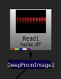
FIGURE 10.21 The Depth channel of a Maya IFF bitmap is converted to the deep-image data format with a DeepFromImage node.
You can examine the “deepness” of any given pixel within a deep image by displaying the Deep Graph (expand the small forward-slash button above the timeline and to the left of the Viewer pane). When you move the mouse across the Viewer, a white line moves across Deep Graph to indicate the pixel depth (distance from camera) (Figure 10.22).
The Deep menu provides a series of nodes designed to work with deep images. Many of the nodes are similar to nondeep Nuke nodes. For example, DeepColorCorrect offers the same Saturation, Contrast, Gamma, Gain, and Offset sliders as the ColorCorrect node. However, several nodes have unique functionality. For example, the DeepTransform node is able to transform a deep image in the X, Y, and Z directions. This allows the 3D object in the image to intersect or move between the 3D objects of another deep image. Such transformations are not available to nondeep images. DeepTransform carries X, Y, Z, and Z-scale parameters. Changing the Z parameter to a negative value pushes the 3D objects of the input further from the camera; positive values bring the objects closer to the camera (Figures 10.23, 10.24, and 10.25). (Note that there is no change in the object scale.) The Z-scale parameter serves as a divisor for the depth value of a pixel; this is useful when converting Depth channels created by different 3D programs. For example, Maya creates a default Depth channel where values change from small negative numbers (close to camera) to 0 (far-clipping plane); hence, changing the Z-scale parameter to —1 makes the Maya Depth channel positive and easier to work with once it’s converted to deep data.
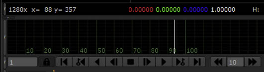
FIGURE 10.22 The Deep Graph. The white line signifies the pixel depth.
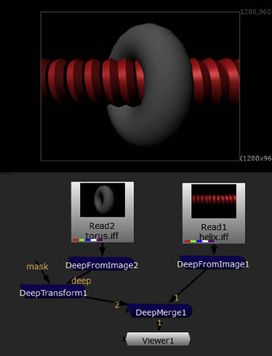
FIGURE 10.23 A DeepTransform node positions a render of a red helix. When the Z parameter is set to 2750, the helix lines up with the center of a torus from a separate deep image. (A DeepMerge node combines the helix and torus render.) A sample script is included as deep.nk in the Chapters/Chapter10/Scripts/ directory on the DVD.
Other useful deep nodes include DeepExpression (allows you to write expressions for deep channels), DeepCrop (crops depth data in front of and behind defined planes), and DeepMerge (merges together deep inputs). For more information on deep compositing theory, visit www.deepimg.com.
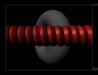
FIGURE 10.24 When the Z parameter is set to 0, the helix is placed in front of the torus.
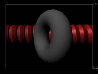
FIGURE 10.25 When the Z parameter is set to 4000, the helix is placed behind the torus.
Introduction to Particles
Nuke v6.3 introduces a set of particle tools. The tools are divided into two menus: Particles and Toolsets > Particles. An easy way to create a particle system is to choose one of the preexisting particle tool sets. For example, to create a snow simulation, follow these steps:
1. Choose Toolsets > Particles > SnowBox. Choose 3D > Scene, 3D > Camera, and 3D > ScanlineRender. Connect the Camera1 node to the Cam input of the ScanlineRender1 node. Connect the Scene node to the Obj/Scn input of the ScanlineRender1 node. Connect a Viewer to the ScanlineRender1 node. In Nuke, the particles simulations occur in a 3D environment.
2. Connect the P_SnowBox1 node to the Scene1 node. The Progress dialog box opens as the particle positions are calculated for the current frame. Change the View Selection menu to 3D. Use the Opt/Alt-mouse button keys to move the default camera back. The P_SnowBox1 node creates a system box that emits numerous snowlike particles (Figure 10.26). Play back the timeline. The particles drift downward. Select the Camera1 icon and interactively move it so that it has a good view of the particles. Change the View Selection menu back to 2D.
3. Open the P_SnowBox1 node’s properties panel. You can adjust the system scale, particle speed, particle scale, particle opacity, and the quality of the turbulence that causes the particles to move in a semi-random fashion.
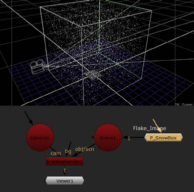
FIGURE 10.26 The SnowBox tool set creates a particle simulation that mimics snow. A sample script is included as snow.nk in the Chapters/Chapter10/Scripts/ directory on the DVD.
To create a particle simulation from scratch, you can follow these basic steps:
1. Choose Particles > ParticleEmitter. Connect the ParticleEmitter node to a Viewer.
2. Connect a geometry node to the ParticleEmitter node’s Emit input pipe. The node emits particles from the surface of the geometry. If the Emit pipe is not connected, particles are emitted along the Y axis. To hide the geometry, change the geometry node’s Display menu to Off.
3. To specify a unique look for the particles, connect a geometry node or Read node with a bitmap to the ParticleEmitter node’s Particle input pipe.
4. Adjust the particles’ emission rate, lifetime, velocity, size, and mass through the ParticleEmitter node’s properties panel.
5. To render the particles from a 2D view, construct a 3D environment with ScanlineRender, Camera, and Scene nodes. Connect the ParticleEmitter node to the Scene node’s input pipe. You can connect shader nodes to the geometry as you would any other 3D scene. To light the particles, add one or more light nodes to the scene.
6. To combine multiple particle simulation, connect the output of one ParticleEmitter node to the Merge input pipe of a second ParticleEmitter node.
7. To alter the speed, direction, and randomness of the particle movement, add one or more force nodes to the scene. For example, connect a ParticleDrag node between the ParticleEmitter node and the Scene node and raise the ParticleDrag node’s Drag value to slow the particles. You can chain several force nodes together.
8. To create the illusion that the particles are bouncing off a surface in the scene, add a ParticleBounce node between the ParticleEmitter node and the Scene node. The ParticleBounce node creates a planar, spherical, or cylindrical boundary, as determined by the node’s Object menu. You must position the boundary to correspond with the surface the particles should “bounce off.” The boundary does not render.
9. To motion blur the particles, raise the Samples parameter in the MultiSample tab of the ScanlineRender node above 1.
For a step-by-step guide to creating an article simulation from scratch, see Tutorial 10 at the end of this chapter.
Image-Based Modeling
Nuke v6.3 includes the Modeler node (3D > Geometry > Modeler), which gives you the ability to create image-based geometry inside the program. Image-based modeling uses photographs or motion picture/video footage to triangulate reference points and thus generate geometry that accurately recreates real-world objects. To apply the Modeler node, you can follow these basic steps:
• Using the CameraTracker node, create a 3D camera to match an image sequence or movie with a moving camera.
• Connect a Modeler node’s Camera pipe to the Camera node and Source pipe to the Read node that carries the image sequence or movie. Switch the View Selection menu to 2D.
• Open the Modeler node’s properties panel. A Modeler toolbar is added to the left side of the Viewer panel. Select the Add Faces tool. Interactively click in the Viewer to add three or more vertices to create a polygon face. Follow the contours of the feature you wish to recreate as geometry. For example, click four times at the corners of a window pane. To close the face, press the Enter key or click the first vertex in the Viewer.
• Move to a different frame on the timeline (preferably one where there’s a significant shift in the camera position). Select the Select/Edit tool. In the Viewer, LMB-drag the vertices to match the current position of the feature you are recreating. For example, move the vertices back to the corners of the window pane. As soon as the node has the positions of vertices for two frames, a 2D polygon face is generated and is visible in the 3D view.
• You can build upon the polygon face by moving, splitting, or extruding it. To split a face, choose the Select/Edit tool, select a polygon edge by LMB-clicking the edge in the Viewer, RMB-click, and choose Split Edge. To extrude a face, choose the Select/Edit tool, press Cmd/Ctrl while selecting the face in the Viewer, and Cmd/Ctrl+LMB-drag the face along the handle. To move a selected face, LMB-drag the face by the handle center. You can continue to adjust vertex positions of all the faces as you move to different frames on the timeline.
For more information on the CameraTracker node, see Chapter 9 or the “CameraTracker User Guide” PDF available at The Foundry website (www.thefoundry.co.uk).
Tutorial 10: Creating a Particle Simulation from Scratch
This tutorial creates a simple particle simulation that includes particle forces and collisions.
1. Create a new script. Choose 3D > Scene, 3D > Camera, and 3D > ScanlineRender. Connect the Camera1 node to the Cam input of the ScanlineRender1 node. Connect the Scene node to the Obj/Scn input of the ScanlineRender1 node. Refer to Figure 10.27 for the final node network. Connect a Viewer node to the ScanlineRender1 node. In Nuke, the particles simulations occur in a 3D environment. Change the View Selection menu to 3D. Interactively move the default camera back.

FIGURE 10.27 The final node network for Tutorial 10.
2. Choose Particles > ParticleEmitter. Connect the ParticleEmitter1 node to the Scene1 node. Play back the timeline. Particles are generated along the Y axis and form a straight line. Choose 3D > Geometry > Sphere. Connect the Sphere1 node to the Emit input pipe of the ParticleEmitter1 node. Return to frame 1 and play back the timeline. Particles are generated from the surface of the sphere (Figure 10.28). Open the Sphere1 node’s properties panel. Change Translate Y to 5. Simplify the sphere by changing Rows/Columns to 6,6. Hide the sphere in the 3D view by changing the Display menu to Off.
3. By default, the particles are white squares. To change the shape, create a second Sphere node and connect it to the ParticleEmitter1 node’s Particle input pipe. Open the Sphere2 node’s properties panel and set Rows/Columns to 3,3. Open the ParticleEmitter1 node’s properties panel. Adjust the Size parameter to scale the particles.
4. At this point, the particles are moving in all directions from the surface of the Emit sphere and are unaffected by any forces. To add gravity to the simulation, choose Particles > ParticleGravity and drop the new node on top of the pipe connecting the ParticleEmitter1 and Scene1 nodes (see Figure 10.27). To increase the gravity’s strength, change the ParticleGravity1 node’s To Y parameter to a larger negative number (e.g., —0.5). When you play back the timeline, the particles arch from the Emit sphere and fall downward (Figure 10.29).
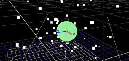
FIGURE 10.28 Particles are emitted from the surface of a sphere.
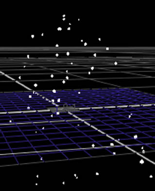
FIGURE 10.29 Particles are pulled downward by the ParticleGravity1 node.
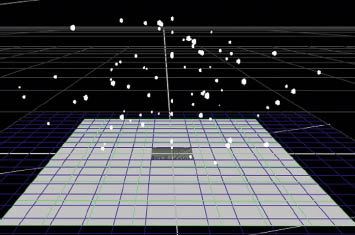
FIGURE 10.30 Particles “bounce” off a card through the assistance of a ParticleBounce node boundary.
5. Choose 3D > Geometry > Card. Connect the Card1 node to the Scene1 node. Scale and rotate the card so that it lies on the “ground” below the particles. Play back the timeline. Note that the particles pass through the card. To create the illusion that the particles are bouncing off the card, choose Particles > ParticleBounce and insert the new node between the Scene1 node and the ParticleGravity1 node. The ParticleBounce1 node creates a planar collision boundary. Through the ParticleBounce1 node’s properties panel, scale the boundary so it matches the scale of a card. Play back the timeline. The particles “bounce” off the card before succumbing to gravity once again (Figure 10.30).
6. Experiment by changing the ParticleBounce node’s Bounce and Friction values, as well as the Lifetime, Velocity, Size Range, and Mass parameters of the ParticleEmitter1 node.
This concludes Tutorial 10. As a bonus step, add lights to the 3D scene, add shaders to the Sphere1 and Card1 nodes, and create a test flipbook render through the 2D view. A sample Nuke script is included as Tutorial10.final.nk in the Tutorials/Tutorial10/Scripts/ directory on the DVD.