
|
|
|
|
Transforming and Keyframing |
|

Compositing programs differ from digital imaging programs in that they are designed for animation. As such, it’s necessary to place keyframes that define the values of parameters at different frames along the timeline. The key-frames define transformations, such as translate, scale, and rotate, and allow various filters to change their qualities over time.
This chapter includes the following critical information:
• Working with bounding boxes
• Transforming outputs
• Keyframing parameters
• Editing animation curves
Bounding, Reformating, and Cropping
The bounding box, visible in the Viewer panels as a dotted white box, defines the area of the frame that the program considers to have valid data. Initially, the bounding box fits itself to the project resolution. The resolution of the bounding box is indicated by an X, Y readout at the top right of the box (Figure 2.1).
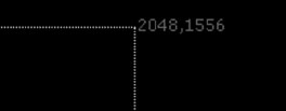
FIGURE 2.1 The X, Y readout of a bounding box. The resolution is 2048 pixels wide 1556 pixels high.
Scaling an Output to the Project Resolution
If an output is connected to the current Viewer, the bounding box snaps to the resolution of the output. If you prefer to maintain the project resolution, you can add a Reformat node to the network. To do so, select the Output node, RMB-click, and choose Transform > Reformat from the Shortcut menu. The output is automatically scaled to fit the project resolution. The output’s original aspect ratio is maintained so that the image is not unduly distorted. For example, applying a Reformat node to a 1920 × 1080 output in a 2048 × 1556 project causes the output to be scaled to 2048 × 1355 (Figure 2.2). In this situation, the top and bottom rows of pixels from the output are streaked vertically to fill the empty areas within the bounding box; you can avoid this, however, by selecting the Reformat node’s Black Outside checkbox.
You can alter the Reformat node’s behavior by changing the Resize Type menu in the properties panel. You can force the rescale to snap vertically by setting the Resize Type to Height or force the output to fit perfectly by changing the Resize Type to Distort. The Reformat node also offers a convenient means to flip an output. Select the Flip checkbox to flip vertically, select the Flop checkbox to flip horizontally, or select the Turn check-box to rotate the output 90 degrees.

FIGURE 2.2 A 1920 × 1080 output is snapped to a 2048 × 1556 project resolution with a Reformat node. A sample Nuke script is included as reformat.nk in the Chapters/Chapter2/Scripts/ directory on the DVD.
Trimming an Output
You can trim the edges of an output by adding a Transform > Crop node. If you raise Box X and Box Y above 0, the left edge and bottom edge are respectively cropped. If you lower Box R and Box T below the default value (which corresponds to the bounding box resolution), the right edge and top edge are respectively cropped (Figure 2.3). The cropped area receives black pixels in the RGB channels and black pixels in the alpha channel, which corresponds to 100% transparency. You can soften the resulting edges by raising the Softness slider. You can snap the resulting cropped output to the bounding box by selecting the Reformat checkbox.

FIGURE 2.3 A 1920 × 1080 output is trimmed with a Crop node. 100 pixels are trimmed from each edge by setting X to 100, Y to 100, R to 1820, and T to 980. A sample Nuke script is included as crop.nk in the Chapters/Chapter2/Scripts/ directory on the DVD.
Translating, Rotating, and Scaling
You can translate, rotate, or scale any node output by connecting the output to a Transform node. You can create a Transform node by RMB-clicking in the Node Graph and choosing Transform > Transform or pressing the T key.
Once a Transform node is connected, a circular handle appears at the center of the output in the Viewer panel (Figure 2.4). You can interactively translate, scale, and rotate the output by LMB-dragging the handle. LMB-dragging the center of the circle translates the output. LMB-dragging the dots lying on the circle scales the output in that direction. LMB-dragging the long line at the right of the circle rotates the output.

FIGURE 2.4 The circular handle provided by a Transform node.
The manipulation of the transform handle remotely changes the parameter values of the Transform node (Figure 2.5). The parameters include Translate X and Translate Y where X runs left/right and Y runs up/down; 0,0 for the translation equates to the default position of the output. You can change what is considered 0,0 and thereby where the handle rests by changing the Center X and Center Y parameters.
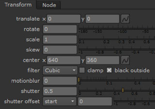
FIGURE 2.5 The parameters of a Transform node.
If an output is translated left/right or up/down without reducing its scale, it overhangs the Viewer bounding box. The Viewer bounding box, which is indicated by a solid line, determines what section of the Viewer output is rendered when a flipbook or a Write node is employed. The resolution of the Viewer bounding box matches the resolution of the transformed output. As such, the overhanging output is cropped.
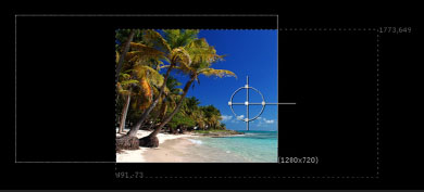
FIGURE 2.6 An output is transformed so that it overhangs the edge of the Viewer bounding box. The portion that overhangs is cropped.
The Transform node also carries Rotate and Scale parameters. In addition, a Skew parameter is provided. Changing the Skew to a nonzero value skews the output into a trapezoidal shape (even through the bounding box remains rectangular).
By default, the Scale parameter carries a single cell and slider, named W (width). If you move the Scale slider, the width and height remain equal, preventing the output from elongating in one direction. If you interactively scale the output, however, the Scale parameter is broken into separate W and H (height) cells. At that point, W and H can carry different values. You can force Scale to carry W and H cells at any time by clicking the Switch Between Single Value And Multiple Values button to the right of the slider (the button features a “2”).
Using Specialized Transform Nodes
Aside from the Transform node, there are several nodes that create unique transformations. They are available through the Transform menu.
CameraShake adds its namesake by moving the output in a seemingly random fashion. The movement is based on a procedural noise. You can add rotation and scale to the shake by raising the Rotate and Scale parameters above 0. To increase the strength of the shake, raise the Amplitude slider. To adjust the “coarseness” of the shake, adjust the Frequency. Lower Frequency values make the individual movements large and slow. Higher Frequency values make the movements small and rapid. To increase the complexity of the movements (where higher-frequency motion is laid over lower-frequency motion) raise the Octaves parameter.
Card3D creates the illusion that the output is a 2D card within 3D space. Hence, the node offers transform parameters that allow you to transform, rotate, and scale the output along X, Y, and Z axes. The output always remains flat, as if it’s a photo postcard (Figure 2.7). (Nuke offers a full 3D environment through specialized camera nodes; these are discussed in Chapter 9.)
Tile allows you to repeat and output in the X and Y directions, much like the UV tiling controls available to a texture in a 3D animation program. You can “zoom” into an output by lowering the Rows and Columns parameters below 1.
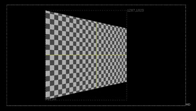
FIGURE 2.7 A checkerboard is rotated with a Card3D node as if it was a 2D card in a 3D space. A sample Nuke script is included as card3d.nk in the Chapters/Chapter2/Scripts/ directory on the DVD.
Several nodes offer redundant transform control. These include Mirror, which allows you to flip or flop an output, and Position, which allows you to move the output in the X and Y directions. Additional nodes are designed for specialized tasks (UV remapping, lens distortion, motion tracking, spline deformation, and HDRI mapping) and are covered in the remaining chapters.
Filter Considerations
Any node that applies a transform includes a Filter parameter (see Figure 2.5). The Filter parameter drives the node’s filter interpolation, which is necessary when the output is rotated, enlarged (upscaled), or reduced (downscaled). The interpolation determines the color values of the resulting pixels. You can roughly divide the filter interpolations into the following three categories:
Nearest neighbor copies the color value of the nearest original pixel. The interpolation is very efficient, but leads to blockiness and stairstepping, whereby diagonal edges are stepped (Figure 2.8). To apply a nearest-neighbor style of interpolation in Nuke, set Filter to Impulse.
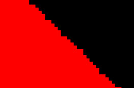
FIGURE 2.8 A red, solid-color bitmap is rotated by 45 degrees with a Transform node. The Filter is set to Impulse, creating stairstepping along the edge.
Bilinear is a type of filter that uses a triangular-shaped curve function. Bilinear filters are able to average the color values of surrounding original pixels by weighting the values based on the distance to the new pixel. Bilinear filters are more accurate than nearest-neighbor filters and produce more subtle transitions between pixels. Bilinear filters are sometimes referred to as tent or Bartlett filters.
Cubic filters build upon bilinear filters by using a bell-shaped curve function. The default Filter setting in Nuke is, in fact, Cubic, which offers the best combination of quality (smooth edges with relatively sharp detail) and efficiency (Figure 2.9).

FIGURE 2.9 Filter is set to Cubic, creating a smoother edge. A sample Nuke script is included as cubic.nk in the Chapters/Chapter2/Scripts/ directory on the DVD.
When examining the results of a particular filter, note the Viewer panel’s zoom setting. For example, in Figures 2.8 and 2.9, the Viewer is set to a 9 zoom so that individual pixels are easily seen. To view an output without any zoom and thus judge it in its native size, set the Zoom dropdown menu at the top right of the Viewer panel to 1. You can interactively zoom in or out by pressing the + or − keys or using a mouse scroll button.
In addition to Cubic, Nuke provides six filter types that use subtle variations of the standard bell-shaped curve. These include Keys, Simon, Rifman, Mitchell, Parzen, and Notch. Of these, Rifman produces the sharpest edges and Notch produces the softest edges (Figures 2.10 and 2.11).

FIGURE 2.10 Filter set to Rifman.
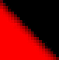
FIGURE 2.11 Filter set to Notch.
When an image is upscaled, new pixels are synthesized and inserted between the original pixels (i.e., the original pixels are padded). When an image is downscaled, pixels must be discarded. To ensure that new or surviving pixels retain accurate colors that represent the original pattern, interpolation filters must be applied. Once again, the cubic family of filters creates the most accurate results.
Bilinear and cubic filters are variations of convolution filters. A convolution filter multiplies the values within an image or output by the values contained in a kernel matrix. A kernel matrix features rows and columns of numbers. Convolution filters are discussed in more detail in Chapter 6.
Keyframing
With traditional, handdrawn animation, a keyframe is a drawing that represents a critical position or pose for a character or object moving through a shot. The phrase includes the word “frame” because that animation requires n number of individual drawings per second and a second is composed of n number of film or video frames. For example, a traditional project might be shot on motion picture film, which operates at 24 frames per second (fps). If the project is animated on 1’s, 24 drawings per second are required, with each drawing exposed for one frame. If the project is animated on 2’s, 12 drawings per second are required, with each drawing exposed for two frames.
In the realm of digital animation, a keyframe is a stored value of a particular parameter of a node at a specific frame on a timeline. This is often referred to as a key and the process of creating keys is keyframing. The keyframe value might take the form of a transformation, whereby the translation, rotation, or scale value along one or more axes (X, Y, Z) is stored. The value might determine the particular intensity of a filter, such as the strength of a blur.
In-betweening
Digital animation offers the advantage of automatic in-between generation. An in-between is a drawing, position, or pose that falls between keyframes. With traditional animation, the addition of an in-between requires an additional drawing. With digital animation, the program provides the in-between values. For example, if you set a keyframe at frame 1 and 10 in Nuke, Nuke creates in-between values for frames 2, 3, 4, 5, 6, 7, 8, and 9. In-between values are created by plotting curves through existing keyframes. Animation curves are discussed in the “Editing in the Curve Editor” section later in this chapter.
Keyframe Theory
Although keyframes are easy to create in Nuke, it may be a challenge to decide where on the timeline a keyframe should be created. The following are several approaches you can take:
Extremes. One common approach to keyframing is to determine the extreme positions of the character, object, or element that is being animated. For example, you may choose to animate a clock pendulum swinging back and forth; if the pendulum is a still image, you would have to create all the motion within Nuke. There are two extreme positions for the pendulum swing: where the pendulum is at its farthest point on the left and where the pendulum is at the farthest point on the right (Figure 2.12). Once the extremes are identified, determine where on the timeline the associated positions occur. The distance between the keyframes determines the speed of the swing. If the pendulum requires 30 frames to move from one extreme to another, it’s moving fairly slow. If the pendulum requires 4 frames to move from one extreme to another, it’s moving fast. Extreme positions for characters often involve the extensions of the appendages (such as arms and legs).
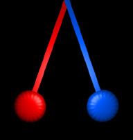
FIGURE 2.12 Two extreme positions for a swinging pendulum. The left extreme is colored red and the right extreme is colored blue.
Story points. Imagine that you are telling a story, even if you are only animating a single shot. Ask yourself what the critical story points are and convert those into keyframe poses or positions. For example, you may choose to animate a ball bouncing; if the ball is a still image, you would have to create all the motion within Nuke. Critical story points for a bouncing ball would include where the ball starts, where it hits the ground at the start of each bounce, where the peak of each bounce is, and where the ball comes to rest (Figure 2.13). Once the critical story points are identified, determine where on the timeline the associated positions occur.
Bisecting. One method that ignores any inherent story is bisecting. Bisecting requires you to set a keyframe at the start and end of the timeline, then at the midpoint, then at halfway points between existing keyframes. For example, with a 100-frame animation, you would set keyframes at 1, 100, 50, 25, 75, and so on. Bisecting can work well when motion of an output is simple or the value change of a parameter is regular and predictable.

FIGURE 2.13 Critical story points for a bouncing ball. From left to right: where the ball starts, where it hits the ground, the peak of the bounce, and where it comes to rest.
Creating and Deleting Keyframes in Nuke
To create a keyframe, follow these steps:
1. Move the time marker to the frame at which you’d like to place a keyframe. Alternatively, you can enter a frame number in the Current Frame Number cell. (For more information on the timeline, see Chapter 1.)
2. Choose the parameter you wish to keyframe. The parameter might be a transform of a Transform node or a specialized parameter of a filter node. Click the Animation Menu button to the right of the parameter and choose Set Key (Figure 2.14). The Animation Menu button features a small, N-shaped curve. The parameter cell turns deep blue to indicate the existence of a keyframe. In addition, a blue line is placed on the timeline at the current frame (Figure 2.15).

FIGURE 2.14 Animation Menu button and its Set Key option.

FIGURE 2.15 Previous and Next Keyframe buttons, plus blue keyframe lines, as seen on the timeline.
3. Move the time marker to a different frame. Change the parameter value by entering a new number into the number cell, moving the slider, or interactively using the handle of a Transform node. As soon as the value changes, a new keyframe is placed automatically at the current frame. Once two keyframes exist, an animation curve is created for the parameter.
You can update an existing keyframe by placing the time marker at the keyframe’s frame number and updating the parameter value. You can delete a keyframe by placing the time marker at the keyframe’s frame number, clicking the corresponding Animation Menu button, and choosing Delete. To remove all the keyframes and corresponding animation curve from a parameter, choose No Animation from the Animation Menu. You can use the Next keyframe and Previous Keyframe buttons available with the playback controls to jump to keyframes (Figure 2.15).
Editing in the Curve Editor
Once a parameter has two or more keyframes, you can edit the resulting animation curve in the Curve Editor. To do so, click the Animation Menu button beside a keyframed parameter and choose Curve Editor. The Curve Editor tab is activated and the corresponding animation curve or curves is displayed.
Curve Editor Overview
The left side of the editor displays a parameter tree (Figure 2.16). The tree includes the node name at the top with each animated parameter and associated channel below. Some parameters, such as Translate, carry two channels: X and Y. (A channel is an attribute that can carry a single animation curve.) Other parameters, such as Rotate, carry a single channel; thus, no additional channels are listed. Even if a parameter carries more than one channel, only the channels that are animated are displayed in the tree.

FIGURE 2.16 The Curve Editor with two animation curves visible.
The right side of the editor features the curve graph. Here, animation curves for selected channels are displayed. Each keyframe is represented by a small dot along a curve. The vertical axis of the graph (the Y direction) represents the value of a parameter channel. The horizontal axis (the X direction) represents time as measured in frames. The curves are threaded through the keyframes; hence, the “curviness” of the curves is dependent on the location of the keyframes.
You can display a single curve in the editor by clicking on the parameter or channel name in the parameter tree. To display multiple curves, Shift-click multiple names. If you switch between curves, you may find that a curve is suddenly out of view. This is due to the values carried by the curves existing in different areas of the graph. You can automatically frame a selected curve, however, by clicking an empty area of the graph and pressing the F key.
To scroll the graph view left/right or up/down, Opt/Alt+LMB-drag. To scale the graph view, Opt/Alt+MMB-drag. To zoom in or out, press the + or − key or use a MMB scroll wheel.
Transforming Keyframes
You can move a keyframe in the Curve Editor graph by LMB-dragging the keyframe point. By default, the keyframe snaps to the nearest whole value along the X axis. To defeat this trait, RMB-click the keyframe point and choose Edit > Frame Snap.
To move multiple keyframes, LMB-drag a selection marquee around the keyframe points. Each selected keyframe point turns white and its associated tangent handles are displayed (tangent handles are discussed in the next section). A transform box is also added (Figure 2.17). You can move the box and keyframes by LMB-dragging the central crosshair. You can also scale the keyframes relative to each other by LMB-dragging any edge of the box. Alternatively, you can Shift-click multiple keyframe points to select them.
When a single keyframe is selected, its values are displayed to the right of the keyframe and take the form of xFrameNumber, yParameterValue (Figure 2.18). You can change the frame number or parameter value in a precise manner by LMB-clicking either readout and entering a new value into the number cell that appears. In addition, the slope value of the tangent handle is indicated by a θ (Theta) value, which is listed beside one or two ends of the tangent handle. For information on tangent manipulation, see the next section.

FIGURE 2.17 Two keyframes are selected. Their tangent handles are drawn as red lines. A white transform box surrounds the keyframes.

FIGURE 2.18 A single keyframe is selected. The frame value (x) and parameter value (y) carried by the keyframe are listed to the right of the keyframe point.
To delete a keyframe, select the keyframe and press the Delete key. To add a new keyframe, select a curve by clicking on it so it turns yellow and Cmd/Ctrl+Opt/Alt-click on the curve. A new keyframe is added where your mouse arrow is positioned. The curve is replotted so that it threads its way through the new keyframe. Adding additional keyframes allows for greater control over the shape of the curve and the resulting animation.
Manipulating Tangents
When a keyframe is selected, its tangent handle is displayed. The tangent determines how the curve flows through the keyframe. Once again, in-between frame values are determined by the program by plotting animation curves. Thus, the shape of an animation curve affects the resulting animation. Hence, the ability to fine tune the tangent handles gives you greater control over the animation process.
You can move a tangent handle by LMB-dragging the dot at either end of the handle. By default, the handle moves like a see-saw. However, you can break the handle into two separate handles, by RMB-clicking over an associated keyframe and choosing Interpolation > Break from the shortcut menu. Once the tangent is broken, you are free to move either side of the handle (Figure 2.19). A broken tangent allows sharp corners to be formed on the curve, which may be useful for creating a sudden change of value (e.g., a transformed output may suddenly change direction). You can “unbreak” a handle by choosing Interpolation > tangent type.
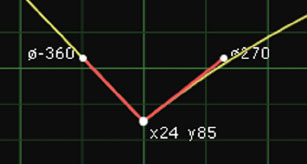
FIGURE 2.19 A broken tangent handle, once manipulated, forms a sharp corner on the curve.
Changing the Tangent Type
By default, Nuke creates curves that smoothly thread through keyframes. You can adjust the way in which the curve flows, however, by changing the interpolation type of one or more of the tangents. To do so, select one or more keyframes, RMB-click in the Curve Editor, and choose Interpolation > tangent type. The following are descriptions of the tangent types:
Smooth is the default tangent type.
Linear forces the curve to move in a perfectly straight line between keyframes (Figure 2.20). This creates abrupt changes in the speed of the parameter value change.

FIGURE 2.20 Three keyframes with Linear tangent interpolation.
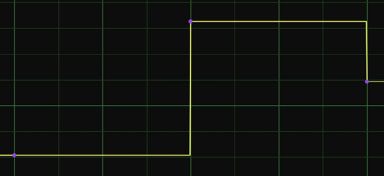
FIGURE 2.21 Same keyframes from Figure 2.20 with Constant interpolation.
Constant creates a stepped curve, where there is no change in the parameter Y value until the next keyframe is encountered (Figure 2.21). If this style of tangent is applied to Translate parameters, the animated element would appear to suddenly jump from one position to the next.
Catmull-Rom, Cubic, and Horizontal offer variations of the Smooth tangent type. Catmull-Rom takes into consideration the Y values of the nearest left and right keyframes; this creates subtle variations in the “curviness” of the curve as it passes through closely spaced keyframes. Cubic matches the tangent slope to the steepest side of the curve as it runs to previous of next keyframes; this can cause the curve to peak at a higher point in Y than the keyframes that lie on its path. (Figure 2.22). Horizontal forces the tangent handles to maintain 0 slope, where the left and right side of the tangent handle has the same position in the Y direction.
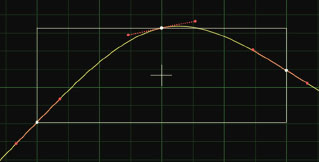
FIGURE 2.22 Same keyframes from Figure 2.20 with Cubic interpolation.
Using the Dope Sheet
The release of Nuke v6.2 introduced the Dope Sheet, which offers an alternative means to adjust when keyframes occur on the timeline. The Dope Sheet appears in its own tab to the right of the Curve Editor. Key-frames are added automatically to the Dope Sheet as they are added to the Curve Editor.
To see specific keyframes in the Dope Sheet, click the Animation Menu button for an animated parameter and choose Dope Sheet from the shortcut menu. The left side of the Dope Sheet contains a parameter tree much like the Curve Editor (Figure 2.23). However, channels are automatically hidden in the tree; to show these, click the + symbol beside each parameter name. For example, clicking the + beside Translate reveals the X and Y channels. The right side of the Dope Sheet contains a keyframe field, where keyframes are indicated as gray markers. The keyframe field indicates time in frames from left to right. There is no Y direction, however, as parameter values are inaccessible in the sheet.

FIGURE 2.23 The Dope Sheet. A Transform1 node is listed with animated Translate X, Translate Y, Rotate, and Scale W (width) parameters. Translate X and Translate Y have three keyframes each, while Rotate and Scale only have two keyframes each.
Manipulating Keyframes
You can select a keyframe marker by clicking it. To move the marker to a different frame, LMB-drag the marker left or right. Note that the parent marker travels with the one you have selected. For example, if you move the W (width) keyframe marker, the parent marker for Scale, as well as the parent marker for the node (such as Transform1) moves in unison (Figure 2.24).
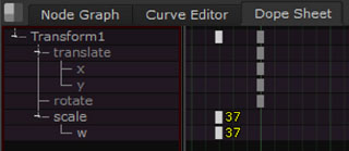
FIGURE 2.24 A Scale W keyframe is selected and moved. The selection is indicated by the white keyframe markers and the yellow frame readout. When the W marker is moved, the parent markers for Scale and Transform1 follow automatically.
To change the view with the keyframe field, use the same key and mouse combinations as you would for the Curve Editor (see the “Curve Editor Overview” section earlier in the chapter). You can select multiple keyframes by Shift-clicking or LMB-dragging a marquee box. You can delete a key-frame by selecting it and pressing the Delete key. You can insert a new keyframe by Cmd/Ctrl+Opt/Alt-clicking in an empty area of the keyframe field.
Adjusting Read Nodes
The Dope Sheet offers the ability to adjust the duration and timeline location of image sequences or video imported through a Read node. To view a Read node in the Dope Sheet, open its properties panel and switch to the Dope Sheet tab. For example, in Figure 2.25, a Read1 node is displayed. The Read1 node carries an image sequence that is numbered 0 to 59 for a total of 60 frames. The parameter tree displays the node name and the File channel. In the keyframe field, the image sequence is represented by a gray horizontal line surrounded by open and close brackets.
You can reposition the sequence/video line by LMB-dragging it left or right. Moving the line to the right causes the sequence/video to occur later on the timeline (Figure 2.26). For example, moving the line so that the open bracket rests at frame 10 means that the sequence/video will not be visible until frame 10. By default, the empty gap on the timeline is filled with a held copy of the first frame of the sequence/video. To avoid this, change the Read node’s Before menu (beside the Frame Range First cell) and After menu (beside the Frame Range Last cell) from Hold to Loop, Bounce, or Black. Loop cycles the sequence/video to fill any timeline gaps. Bounce also cycles the footage, but reverses the frame order with each iteration. Black simply inserts a black frame and does not search for any file; the black frame is given 100% transparent alpha.
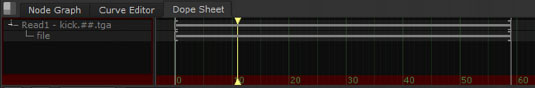
FIGURE 2.25 A 60-frame image sequence is featured in the Dope Sheet. The sequence is numbered 0 to 59, which corresponds to the frame range of the project. The vertical gray lines indicate the frame range start and end.

FIGURE 2.26 The sequence line is moved to the right so that the sequence is not utilized until frame 10 of the timeline. The brackets are moved inwards so only a portion of the sequence is used.
You can trim the sequence/video line so that only a portion is used by the program. To do so, LMB-drag the open bracket to the right and/or LMB-drag the close bracket to the left. In this situation, the frame that rests at the open bracket is repeated to fill the gap between the start of the line and the open bracket. At the same time, the frame that rests at the close bracket is repeated to fill the gap between the end of the line and the close bracket. To alter this behavior, change the Read node’s Before and After menus to Loop, Bounce, or Black.
If the Read node carries a still image, the open and close brackets are provided but no horizontal line appears. The brackets determine how many frames the image is held for on the timeline.
Activating Motion Blur
Motion blur is the streaking of an object as it moves during the exposure of one frame of film or video. If an object moves one foot during the exposure of one frame, the motion blur streak appears one foot long.
By default, animating the transforms of an output in Nuke will not produce motion blur. You can add motion blur, however, by raising a Transform node’s Motionblur parameter above 0. Motionblur sets the sampling rate of the blur, whereby the output is repeated along its motion path (the path drawn in the Viewer that indicates the motion of the output) for the duration of a virtual shutter. The higher the Motionblur value, the smoother and more realistic the blur. In the real world, a shutter is the physical or electronic mechanism of a camera that controls the duration that one frame of film or video is exposed to light. The virtual shutter within Nuke is controlled by the Transform node’s Shutter parameter. By default, Shutter is set to 0.5, which forces the program to start at the current frame and go forward in time 0.5 frames to determine the output’s start and end position along its motion path. The motion blur streak is thus drawn between the start and end position (Figure 2.27).
You can offset the start and end position of the blur by changing the Shutter Offset menu and Shutter Custom Offset cell. For example, if you set Shutter Offset to Centred (centered), the program goes back in time 0.25 frames and forward in time 0.25 frames to determine the start and end position. If you set Shutter Offset to Custom and Shutter Custom Offset to 2, the program goes forward in time two frames to determine the start position. Note that Shutter Custom Offset only functions if Shutter Offset is set to Custom.

FIGURE 2.27 A Transform node has its Motionblur and Shutter parameters set to 1. The transformed spaceship render is blurred along its motion path.
In Part 1 of this tutorial, we set up a new script, imported an image sequence of two characters interacting with an unseen object, imported a 3D render of a stylized heart, adjusted the resolution of the heart render with a Reformat node, and created a simple composite through a Merge node. Part 2 adds keyframe animation to the 3D render, allowing the heart to be kicked out of the frame. In addition, we’ll activate motion blur.
1. Open the Nuke script you saved after completing Part 1 of this tutorial. A sample Nuke script is included as Tutorial1.1.nk in the Tutorials/Tutorial1/Scripts/ directory on the DVD.
2. In the Node Graph, select the Reformat1 node. Press the T key or RMB-click and choose Transform > Transform from the shortcut menu. A Transform1 node is inserted between the Reformat1 node and Merge1 node.
3. Move the time marker to frame 24. This is the frame on which the character wearing the white boots makes contact with the heart during a kick. However, the heart is to too far left to make a solid connection with the boot. While the Transform node is selected and the circular transform handle is visible in the Viewer, interactively move the heart up and to the right. Note that the Transform X and Transform Y parameter cells of the Transform node’s properties panel automatically update with new values. To make the movement more precise, enter 85 in the Transform X cell and 70 into the Transform Y cell. Because the heart render is surrounded by transparent alpha, the bounding box overhang does not matter (Figure 2.28).
4. In the Transform1 node’s properties panel, click the Animation Menu button beside Transform X and Y and choose Set Key. The cells turn deep blue to indicate a keyframe. A blue keyframe line is also placed on the Timeline at frame 24. Move the time marker to frame 27. This is the frame where the kicking boot crosses the corner of the frame. With the Transform1 node selected, interactively move the heart so that it is ahead of the kicking boot and out of frame. While you move the heart, it will remain visible (Figure 2.29); however, when you release the mouse to end the transform, the heart disappears because it is beyond the edge of the frame. A keyframe is set automatically for frame 27. In addition, an motion path line is drawn in the Viewer between the frame 24 position and frame 27 position.

FIGURE 2.28 The heart is transformed to 85,70 in X, Y to better line up with the boot kick.

FIGURE 2.29 The heart is moved past the edge of the bounding box and out of the frame.
5. Play back the timeline. The heart is “kicked” out of frame by the boot. To avoid playing back all 60 frames, you can narrow the timeline by clicking the Frame Range Lock button so that its corners turn red, and enter a new range, such as 20-30, into the Frame Range cell (Figure 2.30). The frame range indicators, which appear as orange triangles on the timeline, move from the default start and end positions to the new range (Figure 2.31). Play back the timeline. The playback is now restricted to the frame range. You can change the Frame Range cell values at any time.
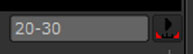
FIGURE 2.30 The Frame Range Unlock button, in an unlocked state (right) and the Frame Range cell (left).
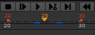
FIGURE 2.31 The frame range indicators (orange) are positioned at frames 20 and 30, while keyframes remain at frames 24 and 27.
6. At this stage, the heart moves in a perfectly straight line due to the existence of two keyframes. You can add an arc to the heart’s animation path by adding a third keyframe. To do so, move the time marker to frame 25. Interactively move the heart so the motion path forms a slight, down-pointing arc (Figure 2.32).

FIGURE 2.32 Close-up of motion path. A third keyframe, at frame 25, allows the path to form a down-pointing arc.
7. When animating, you are not limited to Translate X and Translate Y. In fact, animating the Scale and Rotate parameters can help create more believable motion. To add such animation, return to frame 24 and open the Transform1 node’s properties panel. Click the Animation Menu button beside Scale and choose the Set Key. Do the same for the Rotate parameter. Move the time marker to frame 27. Change the Scale cell to 1.5. Note that the cell changes from a pale blue to a deep blue. While a deep blue color indicates the presence of a keyframe, a pale blue color indicates that the values are derived as an in-between by plotting values on the associated animation curve. Change the Rotate cell to 70. Note that the rotation occurs from the center of the transform handle and not the logical center of the rendered heart. If you wish to rotate the heart from its center, change the Center X and Center Y to 720 and 380, respectively. Ideally, changes to the Center X and Center Y should be applied before setting any keyframes on the node; otherwise, the motion path may be shifted in an undesirable fashion.
8. At this point, there is no motion blur present. You can add blur to the heart by raising the Transform1 node’s Motionblur slider to 1. This significantly slows the playback, at least for the first play through. However, a believable motion blur is created for an otherwise static image (Figure 2.33). To see the result more clearly, you can temporarily hide the various overlays present in the Viewer. To do so, RMB-click in the Viewer and choose Overlay from the shortcut menu. The first time you choose the option, only the motion paths are hidden. The second time you choose this option, all overlays, including bounding boxes and transform handles, are hidden. The third time you choose this option, the overlays return. You can also press the O key.
This concludes Part 2 of Tutorial 1. Save a copy of the script. A sample Nuke script is included as Tutorial1.2.nk in the Tutorials/Tutorial1/Scripts/ directory on the DVD. In Chapter 3, we’ll match the heart to the background through color grading.
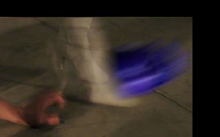
FIGURE 2.33 Detail of motion-blurred heart, as seen on frame 25. The Viewer overlays have been hidden.
Tutorial 2: Flying a Spaceship
Tutorial 2 allows you to adjust previously created animation curves in the Curve Editor. The animation features a 3D render of a spaceship floating over a photographic background.
1. Open the following script on the DVD: Tutorials/Tutorial2/Scripts/Tutorial2.start.nk. The script features two Read nodes. Read1 carries a 60-frame, OpenEXR render of a spaceship. Read2 carries a still photo of an industrial location on the edge of a desert. The spaceship is repositioned through a Transform1 node connected to Read1’s output (Figure 2.34). The output of Transform1 is merged on top of the output of Read2 with a Merge1 node. The result is sent to Viewer1. The project resolution is set to 2048 × 1556. If the output of Merge1 is fit into the Viewer1 panel so that the entire bounding box is visible, the background and spaceship may appear rough. For example, the telephone lines may appear stairstepped. To view the true quality of the output, you must set the Viewer1 panel’s Zoom menu to 1. If you are zoomed in, you can scroll left/right and up/down in the panel by MMB-dragging. You can refit the output image to the Viewer1 tab by changing the Zoom menu to Fit.

FIGURE 2.34 The node network.
2. Play back the timeline. The spaceship moves right to left, finally moving past the edge of the bounding box at the end of the timeline. Select the Transform1 node to display the motion path in the Viewer1 panel (Figure 2.35). Although the 3D render allows the spaceship to slowly rotate in place, the right-to-left motion is provided by the Transform1 node. Examine the Transform1 node’s properties panel. The Translate X, Translate Y, Rotate, and Scale parameters are keyframed animated, as is indicated by the blue number cells.

FIGURE 2.35 Close-up of spaceship render with motion path provided by the Transform1 node.
3. At this stage, the motion path is linear, making the motion of the spaceship very rigid. To alter this motion, you can adjust the animation curves for the Translate X and Translate Y parameters. Click the Animation Menu button beside these parameters and choose Curve Editor from the shortcut menu. To examine the X and Y curves more closely, Shift-select the X and Y channels in the parameter tree of the Curve Editor, click in the curve graph area, and press the F key. The curves are automatically framed (Figure 2.36). The X curve is marked with a small x. The Y curve features a small y. Each curve has three keyframes. (The colors of the curves may vary depending on the version of Nuke you are running.)
4. At this point, the tangent interpolation of the keyframes is linear. To change the interpolations, draw a marquee box around all six keyframes, RMB-click in the curve graph, and choose Interpolation > interpolation type. Try each interpolation type and note the affect the type has on the shape of the animation curves and the shape of the motion path in the Viewer1 panel. When you create a new keyframe, it’s automatically assigned a Smooth tangent interpolation. You can derive the smoothest motion for the spaceship with Smooth, Catmull-Rom, or Cubic interpolation. Catmull-Rom and Cubic will cause the animation path to dip between the first and second keyframes (Figure 2.37). You can adjust the resulting shape, however, by moving the individual X and Y tangent handles.

FIGURE 2.36 The Translate X and Y animation curves.
5. Adjust the tangents of the X and Y curves by selecting a keyframe in the curve graph, clicking the dots on either end of a tangent handle, and LMB-dragging. The goal is to create an animation path that allows the spaceship to smoothly move offscreen (Figure 2.38). Play back the timeline. To see the motion more clearly, hide the motion path and transform handle by pressing the O key twice. (To bring the overlays back, press O a third time.) Due to the large project resolution, the playback will not reach real-time speeds until the second time it loops on the timeline. For more accurate real-time playback, you can create a flipbook. To do so, return to the Node Graph, select the Merge1 node, choose Render > Flipbook Selected from the menu bar, enter 1-60 in the Frame/Frame Range cell of the Flipbook dialog box and proceed to play the timeline of the FrameCycler window. (For more information on the FrameCycler program, see Chapter 1.)
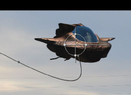
FIGURE 2.37 The Cubic tangent interpolation causes the motion path to dip between the first and second keyframes.

FIGURE 2.38 The adjusted X and Y curves and the resulting motion path.
6. Although the spaceship exists as a rendered image sequence, it does not include motion blur. Although 3D programs such as Auotdesk Maya can create motion blur, it must be activated (in this case, it wasn’t). Because the right-to-left motion of the spaceship is provided by the Transform1 node, you can add motion blur in the composite by raising the Transform1 node’s Motionblur parameter to 1. Although the resulting blur is relatively subtle, it will help with the realism of the scene (Figure 2.39).

FIGURE 2.39 Motion blur is activated for the Transform1 node.
This concludes Part 1 of Tutorial 2. Save a copy of the script. A sample Nuke script is included as Tutorial2.1.nk in the Tutorials/Tutorial2/Scripts/ directory on the DVD. In Chapter 3, we’ll adjust the elements though color grading.