|
|
|
|
Alpha Mattes, Merging, and Rotoscoping |
|

Compositing necessitates the combination of bitmaps, image sequences, videos, and/or procedurally-generated patterns. Whereas a layer-based program simply stacks layers with preference to upper layers, Nuke combines inputs through various “merge” nodes. Regardless of the compositing program used, a layer or input’s alpha channel must be considered as it carries pixel transparency information. In Nuke, if an input does not carry an alpha channel, you can synthesize one by creating an alpha matte. You can generate such a matte by manipulating RGB information, targeting a specific color with a chroma key node, or drawing a mask with a rotoscoping node.
This chapter includes the following critical information:
• Working with alpha
• Combining inputs with merge nodes
• Generating mattes
• Rotoscoping masks
Understanding Alpha and Premultiplication
In the realm of digital image manipulation, alpha is a channel that stores transparency information. The transparency information is often referred to as a matte, where the matte carries grayscale values. The values run from 0-black (equal to 100% transparency) to 1-white (equal to 100% opaqueness). Alpha is necessary when compositing various elements on top of each other without having higher elements completely obscuring the lower ones. With a Nuke Merge node, the input A pipe is the “higher” input, while the input B pipe is the “lower” input.
You can examine an alpha channel in Nuke by pressing the A key while the mouse is over the Viewer panel (Figure 4.1). While some image formats carry an alpha channel, others do not. By the same token, image formats that support alpha may not include the alpha information. For example, a Targa render generated by Autodesk Maya will most likely include an alpha channel. However, a TIFF scan of motion picture film will not include alpha. Nevertheless, you can add an alpha channel to any output within Nuke at any time. For more information on image formats and whether they support alpha, see Chapter 1.

FIGURE 4.1 Close-up of the alpha channel carried by the spaceship render used for Tutorial 2. The majority of pixels are 0-black or 1-white with a few pixels along the ship edge carrying midrange values such as 0.5. The render was generated with Autodesk Maya.
Premultiplication Overview
Premultiplication is an optional process whereby the RGB values of a digital image are multiplied by the alpha values within the same image. For example, if a pixel in the red channel has a value of 0.8 and the alpha value of the same pixel has a value of 0.5, the resulting premultiplied red channel value for the pixel is 0.4. Ultimately, premultiplication speeds up compositing calculations. If premultiplication is interpreted correctly by a compositing program, matte edges appear clean. (Matte edges occur along the edges of objects where the transparency transitions from 100% transparency to 100% opaqueness.) If premultiplication is incorrectly interpreted, a gray line often appears in RGB along the object edge; this is particularly evident when motion blur is present.
For example, in Figure 4.2, a render of a 3D primitive is merged over a white background. The Premultiplied parameter carried by the render’s Read node remains deselected. The motion-blurred edge of the render picks up a gray cast, which interferes with the texture detail along the edge. In this situation, an empty 3D background influences the semi-transparent pixels along an object edge. 3D programs, such as Autodesk Maya or 3ds Max, assign the black RGB values to empty space (although you can change the color if you wish). The programs also offer the option to render an alpha channel in addition to the RGB channels; the renders are automatically premultiplied.

FIGURE 4.2 Close-up of 3D render in Nuke with alpha left in a unpre-multiplied state. The motion-blurred edge picks up a gray cast. A sample script is included as unpremultiplied.nk in the Chapters/Chapter4/Scripts/ directory on the DVD.
Premultiplying and Unpremultiplying in Nuke
Nuke automatically recognizes the alpha channels of imported images. However, premultiplication is not recognized unless you select the Read node’s Premultiplied checkbox. The Premultiplied parameter adds the following steps to the Read node interpretation:
1. Divides the color values by alpha values (unpremultiplies).
2. Applies the color space conversion as determined by the Colorspace parameter.
3. Remultiplies the color values by alpha values.
The extra steps guarantee the proper color values appear along the matte edges.
Additionally, Nuke supplies Premult and Unpremult nodes (in the Merge menu) to premultiply or unpremultiply any output. Occasionally, you will need to manually premultiply or unpremultiply an output so that the alpha values are correctly interpreted. For example, the Erode node requires pre-multiplication to function properly. This is demonstrated in “Tutorial 3: Removing an Imperfect Greenscreen” at the end of Chapter 5. Additional examples are included throughout this book.
Using the Merge Node
The Merge node is tasked with merging inputs. Whereas a layer-based compositing program, such as After Effects, recognizes a dominate layer by its top-most position in the layer stack, the Merge node gives preference to input A. Therefore, you may consider Input A the “top” and Input B the “bottom.”
A Merge node can accept more than two inputs (Figure 4.3). When you connect an additional input, the input pipes are relabeled; input A becomes input A1 and any additional inputs are labeled A2, A3, A4, and so on (input B remains the same). The input with the highest A number, such as A4, is given preference and becomes the “top” input. Note that the input pipe stub at the left side of the node icon carries the next highest input A; for example, if three input connections exist, the input pipe becomes A3.

FIGURE 4.3 A merge node with three input connections. In this example, A2 is the “top” input, A1 is the “middle” input, and B is the “bottom” input.
Choosing a Math Operation
The way in which inputs are combined is determined by the Merge node’s Operation menu. The Operation menu applies a specific mathematical operation to determine how the pixel values of the various inputs are added, subtracted, multiplied, or averaged. The Operation menu is set to Over by default. If you are working with premultiplied inputs, you can write the Over operation as
![]()
If the inputs remain unpremultiplied, the formula changes to
![]()
In this case, A is the red, green, or blue value of a pixel in input A; B is the red, green, or blue value of the matching pixel in input B (the operation is applied to one color channel at a time); a is the alpha value of the same pixel in input A; b is the alpha value of the same pixel in input B; and C is the output value of the merged pixel. Hence, A occludes B unless a is less than 1. For example, if A is 0.5, a is 0.5 (50% transparency), B is 0.8, and b is 1 (0% transparency), the following math occurs:
![]()
There are 30 operations available through the Operation menu. To display the mathematical formula for each, hold your mouse over the parameter name until the help dialog appears (Figure 4.4). Of the Operations, Over is used the most often. Other common operations include Screen, Multiply, Min, and Max. Various operations are demonstrated through the remainder of this book. To see the result of a particular operation, you can change the Operation menu at any time.

FIGURE 4.4 The Operation parameter help dialog. Mathematical formulas for each option are written out (* is the same as ×).
Mix Slider and Channel Menus
The Mix slider, located along the bottom of the Merge node’s properties panel (Figure 4.5), determines the contribution strength of input A (and A1, A2, A3, and so on). In essence, input A’s alpha value is multiplied by the Mix value. Hence, if Mix is set to 0.5, an otherwise opaque input A receives 50% transparency.

FIGURE 4.5 Merge node properties panel with Channels parameter sets and Mix slider.
Input A, input B, and the node output each receive a Channels parameter set in the Merge node properties panel (Figure 4.5). By default, the RGBA channels of the inputs are accepted by the node. By default, the node outputs RGBA. However, you can pick and choose which channels are accepted as input or as output by changing the Channels menu (the left menu that defaults to Rgba); selecting or deselecting the Red, Green, or Blue parameter checkboxes; and/or changing the Additional Channel menu (the right menu). For example, you can deselect Red, Green, and Blue and leave the Additional Channel menu set to Rgba.alpha; thus only the alpha channel is processed. Note that all A inputs (A1, A2, A3, and so on) are affected equally by a single A Channels parameter set.
Chaining Merge Nodes
As an alternative to connecting more than two inputs to a Merge node, you can chain two or more Merge nodes together. For example, in Figure 4.6, two spaceship renders are added to a background with the aid of two Merge nodes. The output of Merge1 is connected to the input B of Merge2. This offers the immediate advantage of providing two Mix sliders and two A Channels parameter sets. Therefore, the opacity and utilized channels of each render is independent. If the renders are connected to input A1 and input A2 of a single Merge node, they would share a single Mix slider and a single A Channels parameter set.
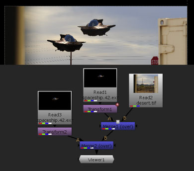
FIGURE 4.6 Two Merge nodes are chained together.
Hooking Up a Mask
Many nodes in Nuke, including the Merge node and various filter nodes, carry a Mask input (Figure 4.7). Initially, the input is drawn as a pipe stub at the right side of the node icon. With a Merge node, the Mask input determines where input A will appear. The node carries this out by multiplying the alpha values within the Mask input by the alpha values within input A. If a pixel in the Mask input has a value of 0, the corresponding pixel within the input A alpha channel receives a value of 0; this causes the input A pixel to become 100% transparent. With a filter node, such as Blur, the Mask input limits where the filter effect occurs. For example, you can limit a blur to a small area of the frame. Note that the Mask input affects all A inputs equally (A1, A2, A3, and so on).

FIGURE 4.7 Merge node Mask input pipe.
Whereas an alpha channel is often referred to as an alpha matte or a channel that carries matte information, a mask is a device that generates a matte. The device may take the form of a bitmap, a procedural texture, or a bezier shape drawn within the compositing program. If a bitmap is used as a mask, it need not contain shades of gray. In fact, you can reuse the RGB information of a bitmap to control where a filter node has the greatest impact. For an example, follow these steps:
1. Create a new Nuke script. Create a Read node. Import a bitmap or image sequence that features an area with a saturated color, such as red. You can use the lipstick.tif bitmap included in the Chapters/Chapter4/Bitmaps/ directory on the DVD. The included bitmap features an actress wearing bright red lipstick (Figure 4.8). Connect a Viewer to the Read1 node.

FIGURE 4.8 The lipstick.tif bitmap features an actress with bright red lipstick.
2. With the Read1 node selected, choose Color > Saturation. Change the Saturation parameter to 0. The image turns grayscale. Create a new Read node. Import the same bitmap into the Read2 node. Connect the Mask input of the Saturation1 node to the output of the Read2 node. You can do this by LMB-dragging the pipe stub at the right side of the Saturation1 node icon and dropping it on top of the Read2 icon. Use Figure 4.9 as a reference for the final node network.
3. At this point, a red error message appears at the top of the Viewer tab: Nonexistent channel used for mask. By default, any node that carries a Mask channel takes information from the input’s alpha channel. Because the lipstick.tif bitmap does not carry an alpha channel, there is no information to read. To solve this, open the Saturation1 node’s properties panel and change the Mask Channel menu to a channel that exists, such as Rgba.red (Figure 4.10). Once a valid channel is selected, the error message is removed. The heaviest areas of desaturation thus occur in areas of the Mask input that carry the highest values. If the Mask Channel menu is set to Rgba.red, the lips are thus desaturated and lose their redness (Figure 4.11). Change the Mask Channel menu to Rgba.green and Rgba.blue channels for differing results. A sample script is included as mask.nk in the Chapters/Chapter4/Scripts/ directory on the DVD.
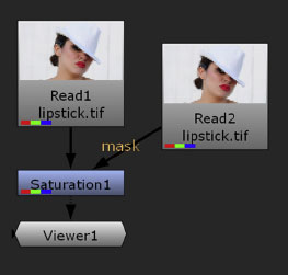
FIGURE 4.9 Node network with Saturation1 node utilizing the Read2 output as a mask.
FIGURE 4.10 Saturation1 node’s Mask Channel menu changed from default Rgba.alpha to Rgba.red.

FIGURE 4.11 The lips are desaturated as the desaturation is targeted at areas with intense red through the red channel mask.
Note that the presence of an input A alpha channel may affect the resulting merge. For example, in Figure 4.12, input A (a photo of a field) is masked with a black-and-white bitmap featuring a squiggled line. The Merge node’s Mask Channel menu is set to Rgba.red. Input A carries a solid-white alpha channel. Hence, input A is cleanly masked. The Merge node merges the cutout input A over a solid red color provided by a Constant node. If input A is switched to an input that does not possess an alpha channel, cut-out input A becomes semi-transparent (Figure 4.13). Nevertheless, it is possible to avoid the transparency by changing the Merge node’s Operation. For example, setting the menu to Copy returns the opaqueness to Input A.

FIGURE 4.12 Input A (a photo of a field) carries an alpha channel and thereby is cleanly masked over a red Constant. A sample script is included as alphamask.nk in the Chapters/Chapter4/Scripts/ directory on the DVD.
The Merge node’s Mask parameter is selected automatically when a Mask input is connected to another node. You can invert the Mask input by selecting the Invert parameter (see Figure 4.10). Bezier shapes, used as masks, are detailed in the “Rotoscoping” section later in this chapter. Step 3 of Tutorial 2, featured at the end of this chapter, uses a procedural Noise node as a mask.
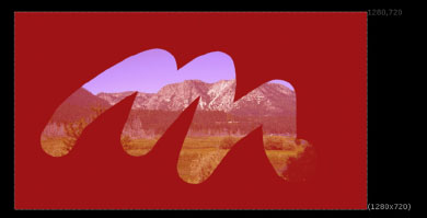
FIGURE 4.13 Input A, lacking an alpha channel, becomes semi-transparent when merged over the Constant. A sample script is included as noalphamask.nk in the Chapters/Chapter4/Scripts/ directory on the DVD.
Pulling a Matte
In many situations, the output that requires a matte contains all the necessary information needed to create that matte. This approach is often called pulling a matte. Although you can utilize red, green, and blue channel information, as is demonstrated earlier in the section “Hooking Up a Mask,” you can also use luminance information. Such a pulled matte is often referred to as a luma matte. For example, in Figure 4.14, a matte is pulled from a bitmap photo featuring silhouetted dancers against a bright set of windows.
With this example, the following steps occur:
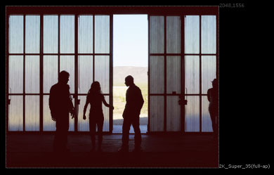
FIGURE 4.14 A matte is pulled from the luminance information contained within a bitmap photo of silhouetted dancers. As a result, the red of a Constant node appears in the darkest areas.
1. The color space of the bitmap is interpreted as Linear through the Read1 node.
2. The color space is converted to L*a*b* through the Colorspace1 node (Figure 4.15).
3. The contrast of the luminance channel is increased by the ColorCorrect1 node.
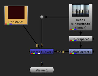
FIGURE 4.15 The node network that creates the luma mask.
4. The luminance channel is used as matte information through the Mask connection of the Merge1 node.
5. The original bitmap is merged with a dark red color provided by the Constant1 node. The dark red appears in the silhouetted areas of the bitmap but does not affect the bright areas of the windows or the doorway. To ensure that the Mask input uses the luminance information, the Mask Channel menu of the Merge1 node is set to Rgba.red. (When the color space conversion is carried out, L* [luminance] is carried by the red channel; for more information on L*a*b* color space and the Colorspace node, see Chapter 3.)
If you wish to see what the luma matte looks like, connect Viewer1 to the ColorCorrect1 node and press the R key in the Viewer panel. A sample script is included as luma.nk in the Chapters/Chapter4/Scripts/ directory on the DVD. The chroma key process, whereby you convert a specific color to matte information, is a form of matte pulling and is discussed in Chapter 5.
Specialized Merge Nodes
In addition to the Merge node, Nuke provides several nodes designed for specialized merging. These are described briefly here.
Blend outputs the weighted average of two or more inputs. Each input pipe is consecutively numbered and receives a matching weight slider in the node’s properties panel. The higher the slider value of an input, the more biased the weighting is toward it and the more opaque the input appears.
Dissolve also outputs the weighted average of two or more inputs (numbered 0, 1, 2, and so on). The Which parameter determines the weighting and runs from 0 to the highest input value. For example, if there are three inputs, the parameter runs from 0 to 2. If the Which slider is set to 0, the 0 input occludes the other inputs. If the slider is set to 1.5, the 1 and 2 inputs are averaged.
TimeDissolve, in contrast, only accepts two inputs (A and B). The two inputs are averaged. However, the weighting is controlled by an interactive curve (Figure 4.16). Time runs along the left/right X axis of the curve graph; the time range uses a normalized 0-to-1 scale, where you control the start and end frame through the In and Out parameters. The up/down Y axis also runs from 0 to 1 and represents the weighting. If a curve point sits at 1, input B occludes input A. If a curve point sits at 0.5, a 50% mixture of both inputs results. You can edit the curve as you would any other curve in the Curve Editor.
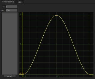
FIGURE 4.16 The curve graph of a TimeDissolve node. A new curve point is inserted at 0.5 in X. The curve is reshaped so that the node dissolves from input A to input B to input A once again. A sample script is included as timedissolve.nk in the Chapters/Chapter4/Scripts/ directory on the DVD.

FIGURE 4.17 A 3D render is merged over a background with an AddMix node.

FIGURE 4.18 The AddMix A curve is bowed upward to give the A alpha channel midrange greater intensity. The B curve remains in its default state.
AddMix provides two interactive curves. The input A alpha is multiplied by the A curve and the input B alpha is multiplied by the B curve before the two inputs are added together. The interactive curves allow you to wield greater control over the edges of the output alpha matte. For example, in Figure 4.17, a render of a moving 3D primitive is merged over a background sky. If the A curve of the AddMix node is altered so that the midrange of the input A alpha is given reduced values (Figure 4.18), the motion-blurred edge of the primitive becomes more transparent and thus more subtle (Figure 4.19). Moving an A curve point upward in the graph causes an alpha value reduction, while moving a point downward has the opposite result. You can edit the curve as you would any other curve in the Curve Editor. Note that the AddMix node carries a Premultiplied parameter, which is deselected by default. A sample script is included as addmix.nk in the Chapters/Chapter4/Scripts/ directory on the DVD.

FIGURE 4.19 The altered A curve has greater transparency along the motion-blurred edge.
CopyRectangle cuts a rectangular hole into input B, thus allowing input A to show through. You can interactively move and scale the rectangle in the Viewer.
KeyMix cuts a hole into input B, allowing input A to show through. However, KeyMix requires that you connect a mask to its Mask input to define the cut region.
MergeExpression allows you to write an expression for specific channels. The properties panel appears identical to the Expression node (Color > Math > Expression). However, the MergeExpression node carries two input pipes (A and B), which you can reference within the expressions. Expressions are explored in Chapter 10.
Rotoscoping
Rotoscoping is any process that generates an animated mask, whereby the mask is converted to an alpha matte. The mask changes with each frame and thus follows the contours of a specific object. For example, you might rotoscope an actor to separate him or her from the background. With a digital compositing program, rotoscoping may take the form of an animated spline or hand-painted mask shapes. Rotoscoping is an important compositing technique; in fact, it’s often used in combination with other matte-generation approaches, such as chroma keying (discussed in Chapter 5). Before the advent of digital image manipulation, rotoscoping required the tracing of motion picture film frames on paper. Nuke provides two nodes for the purpose of rotoscoping: Roto and RotoPaint.
Roto Node
The Roto node is designed for the specific task of rotoscoping. The node allows you to interactively create spline-based shapes, which are filled automatically to create matching alpha mattes. To apply the node, follow these general steps:
1. With no nodes selected, choose Draw > Roto (or press the O key in the Node Graph). A Roto node is created and a special Roto toolbar is added to the left side of the Viewer panel. From top to bottom, the toolbar includes a selection tool set, a points tool set, and a shape tool set (Figure 4.20).
2. With the Bezier tool selected (the Bezier tool is selected by default when a new Roto node is created), draw a bezier shape in the Viewer by clicking around the contour of the object you wish to separate. (If the Viewer does not display the output you wish to rotoscope, temporarily connect the Viewer to that output.) Each time you click, a point is deposited. In the same way the points of a curve in the Curve Editor define the curve’s shape, the points of a Roto bezier define the bezier shape. For the bezier to create a functioning alpha matte, the bezier must be closed. That is, the last point must be placed where the first point lies. When you position the mouse pointer over the first point, the pointer displays a small circle, indicating that an additional click will close the bezier. Alternatively, you can press the Enter key to force a closure; Nuke automatically adds a bezier segment between the first point and the last point deposited.
3. Once the bezier shape is closed, it’s filled with white in the RGB and alpha channels. To avoid obscuring the RGB channels with the white fill, you can temporarily reduce the Roto node’s Opacity parameter to 0. (The Opacity parameter affects the RGB and alpha channels equally; to utilize the alpha channel as an alpha matte, Opacity must be left at 1.) If the Roto node is connected to a Viewer, you can examine the alpha channel by placing the mouse in the viewer and pressing the A key. The interior of the shape receives an alpha value of 1 (opaque), while the space around the shape receives an alpha value of 0 (transparent). You can connect the output of the Roto node to any other node that may benefit from the alpha matte. For example, you can connect the Roto output to the Mask input of the Merge node. The Merge node’s input A is thus cut by the matte (Figure 4.21).
FIGURE 4.20 Roto node toolbar.

FIGURE 4.21 An alpha matte, generated by a Roto node, is connected to the Mask input of a Merge node. The Merge node’s input A is thus cut by the matte; this maintains the field and mountain but removes the sky. A sample script is included as roto.nk in the Chapters/Chapter4/Scripts/ directory on the DVD.
For a working example of the Roto node, see Tutorial 1 at the end of this chapter.
Editing a Bezier and Using B-Splines
You can edit an existing bezier shape in the following ways:
• To add a point to an existing bezier shape, click the bezier so that the existing points are visible and Cmd/Ctrl+Opt/Alt-click a bezier segment. Alternatively, switch to the Add Points tool available through the center Roto tool set.
• To delete a point, select the point with the Select All tool (available through the top Roto tool set) and press the Delete key; a selected point is indicated by a small line running perpendicular to the surrounding segments. Alternatively, switch to the Remove Points tool available through the center tool set.
• To curve a point by inserting a tangent handle, select the point with the Select All tool and press the Z key. Alternatively, switch to the Curve Points tool available through the center tool set. You can rotate the tangent handle by LMB-dragging either tangent end. You can lengthen or shorten the tangent handle by dragging a tangent end in or out. To move one tangent end independent of the other, Cmd/Ctrl-drag.
• To cusp a point and thereby create a sharp corner, select a point and press Shift+Z. Cusped points are created by default when you draw the bezier shape. Alternatively, switch to the Cusp Points tool available through the center Roto tool set.
By default, the Roto node creates bezier shapes. However, you can also create B-spline, ellipsoid, or rectangular shapes. To create an ellipse or rectangle, switch the bottom Roto tool set to the namesake shape and LMB-drag in the Viewer. The resulting ellipse or rectangle is closed and carries four points that are either smoothed or cusped. You can edit the ellipse and rectangle as you would any other bezier shape. To create a B-spline shape, switch the bottom tool set menu to B-Spline and click in the Viewer. B-splines differ from beziers in that their points lie off the segments (much like a NURBS curve in Maya). You can add or delete points in the same way you would with a bezier shape. However, B-spline points generate smooth shapes that cannot maintain sharp corners (Figure 4.22).
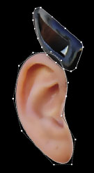
FIGURE 4.22 A B-spline shape (bottom, around ear) is combined with a bezier shape (top, around clip). A sample script is included as bspline.nk in the Chapters/Chapter4/Scripts/ directory on the DVD.
Combining Multiple Shapes
You can draw multiple shapes while using a single Roto node. To add an additional shape, click a shape tool, such as Bezier, in the Roto node toolbar and deposit points in the Viewer. Each shape is listed in the Curves section of the Roto tab of the node’s properties panel (Figure 4.23). The Curves section allows you to hide shapes, lock shapes (prevent edits), change the handle color (color of the shape curve), change the render color (the shape fill color), invert the alpha matte, choose a blending mode (the mathematical way in which shapes are combined), and activate motion blur for animated shapes.
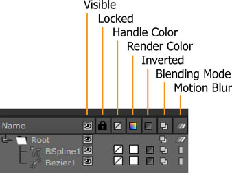
FIGURE 4.23 The Curves section of a Roto node’s properties panel.
By default, the Roto node’s blending mode is set to Over. This is identical to the Over operation used by the Merge node. You can change the blending mode to other common operations by clicking the Blending Mode icon in the Curves section. (For more information on operations, see the “Choosing a Math Operation” earlier in this chapter.) For example, if you need to cut a hole into a shape, draw a smaller shape and set the new shape’s blending mode to Exclusion (Figure 4.24).

FIGURE 4.24 A hole is cut into a shape by setting a smaller shape’s blending mode to Exclusion. A sample script is included as exclusion.nk in the Chapters/Chapter4/Scripts/ directory on the DVD.
You can delete, copy, or paste a shape by RMB-clicking the shape name in the Curves section. You can rename a shape by double-clicking the shape name and entering new text into the name field. The order in which the shapes appear in the Curves section affects the way in which the shapes are blended together. The top-most shapes win out over lower shapes much like a layer stack in Adobe Photoshop or After Effects. You can reposition a shape in the stack by selecting and LMB-dragging the shape name up or down. Selected shapes are indicated by an orange bar.
Feathering a Shape
Initially, the transition from 0-transparent pixels and 1-opaque pixels in the generated alpha matte is hard. You can soften this transition, however, by adjusting a point’s feather. To do so, select the point. A small line appears perpendicular to the segments that lie to either side of the point. Click on the small line and drag outward. A feather point and dotted feather segments appear (Figure 4.25). (If the line is not visible, RMB-click over the point and choose Increase Feather from the menu.) The space between the feather segments and the original segments becomes a soft transition. You can pick and choose which points to feather; in addition, each point can carry a unique feather. The feather points carry their own tangent handles, which you can adjust separately. You can remove a feather from a point by switching to the Remove Feather tool through the center Roto tool set and clicking on the point in the Viewer. You can also remove a feather by RMB-clicking over the point and choosing Reset Feather from the menu. The ability to feather the shape is extremely useful when rotoscoping an object that is motion-blurred.
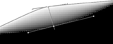
FIGURE 4.25 Close-up of a shape feather. The feather point (bottom) creates a 12-pixel transition from opaque alpha to transparent alpha at the widest span of the feather.
Adjusting the Matte Edge and Transforms
You can alter the overall quality of a shape’s alpha matte edge by changing the Feather and Feather Falloff parameters. To do so, first select the shape name in the Curves section of the Roto node’s properties panel. Feather controls the uniform softness, where higher values create a blurrier edge. Feather Falloff sets the rate of opacity change at the matte edge, where higher values create a more gradual transition from opaque alpha to transparent alpha.
You can change a shape’s translation, rotation, scale, and skew through the Roto node’s Transform tab. Once again, you must first select the shape name in the Curves section in the Roto tab. If you animate the shape, either through the Transform tab or by animating the positions of individual points (see the next section), you can adjust the resulting motion blur through the Shape tab.
Animating a Shape
When a bezier or B-spline shape is closed, it creates an alpha matte. The matte does not change over time. This is often useful for creating a matte for an object or objects that do not move. Such a matte often takes the form of a garbage matte, whereby unwanted objects in a shot are quickly deleted. For example, you might create a garbage matte to remove lighting equipment that appears along the edges of a greenscreen plate. In contrast, rotoscoping requires that the matte changes over time. This is necessary when creating a matte for a moving object, vehicle, or character. When using the Roto node, you can create an animated shape and matching animated matte with a few additional steps:
1. As soon as a shape is created with the Roto node, a keyframe for the shape is placed on the timeline for the current frame. This is indicated by a blue line. Move the time marker to a different frame. Interactively move points in the Viewer to match the contour of the object you are trying to rotoscope. Feel free to adjust tangents and feathering. As soon as a point is moved or adjusted, the Roto node creates a new keyframe. Note that each shape carried by a Roto node carries a unique set of keyframes. If you select a shape in the Viewer, the corresponding shape name is selected in the Curves section of the properties panel; if you select the shape name in the panel, the shape is selected in the Viewer.
2. Play back the timeline. The Roto node creates in-between positions for the shape so that it can successfully morph between the contours you defined. Continue to move the time marker to different frames and continue to adjust the shape. You can move all the points of the shape as a single unit by switching to the Select Points tool through the Roto toolbar top menu, LMB-dragging a selection marquee in the Viewer, and LMB-dragging the resulting transformation handle. You can delete a keyframe by moving the time marker to the appropriate frame and clicking the Delete Key button in the properties panel (beside the Spline Key parameter). Note that the Spline Key cell appears dark blue when the timeline rests on a keyframe and appears light blue when the program is creating an in-between position for the shape. The total number of keyframes created for a shape is indicated by the cell to the right of the word “of.”
In general, it’s not necessary to create a keyframe for every single frame of the timeline. However, the number of keyframes required is dependent on the complexity of motion you are rotoscoping. In addition, it’s not necessary to create a single shape for the rotoscope. You can break down an object into smaller, overlapping shapes to make the process easier. For example, if you are rotoscoping an actor, you can create one shape for the head, one shape for the neck and torso, and extra shapes for the arms and legs.
RotoPaint Node
The RotoPaint node includes the functionality of the Roto node but adds the ability to interactively paint strokes. The strokes are based on a spline curve; however, you can determine the size, color, and softness of the stroke. When you create a RotoPaint node (Draw > RotoPaint), it adds its own toolbar to the left side of the Viewer tab. The top three tool sets are identical to the Roto node (see the “Roto Node” section earlier in this chapter). However, four new tool sets are added. From top to bottom, these are Brush/Eraser, Clone/Reveal, Blur/Sharpen/Smear, and Dodge/Burn (Figure 4.26).
FIGURE 4.26 Unique RotoPaint tool sets.
Using the Brush
To use the Brush tool with the RotoPaint node, follow these steps:
1. Select the output you wish to rotoscope and choose Draw > RotoPaint. The output is connected to the Bg input of the new RotoPaint node. Connect the output of the RotoPaint node to a Viewer. The RotoPaint toolbar is added to the left side of the Viewer panel. In addition, a settings bar is added to the top of the view area.
2. Select the Brush tool through the left toolbar. The tool features a paintbrush icon. The settings bar updates to reveal controls that determine the color, blending mode, opacity, size, and hardness of the brush stroke (Figure 4.27). The right-most menu controls the lifespan and defaults to Single, which means that the stroke will only appear at the current frame. If you wish the stroke to last for the entire duration of the timeline, switch the menu to All. You can also choose a specific frame range by switching the menu to Range. LMB-drag in the Viewer to draw the stroke. When you release the mouse button, the stroke is completed and is listed in the Curves section of the RotoPaint node’s properties panel as Paintn.
FIGURE 4.27 The RotoPaint settings bar, as seen when the Brush tool is selected.
3. You can delete, copy, paste, change the stack order, change the blending mode, or invert the alpha matte of any stoke in the Curves section. To edit the stroke qualities of an existing stroke, select the stroke name in the Curves section and switch to the Stroke tab. The tab includes Brush Size, Brush Hardness, and Source parameters. Source controls the color of the stroke and has the same functionality as the Source parameter in the Shape tab. You can change the stroke’s lifespan through the Lifetime Type menu of the Lifetime tab.
4. The stroke appears in the RGB and alpha channels. To see the alpha channel, disconnect the Bg pipe and press the A key while the mouse is in the Viewer. You can connect the output of the RotoPaint node to any other node that may benefit from the alpha matte. For example, you can connect the Roto output to the Mask input of the Merge node. The Merge node’s input A is thus cut by the matte (Figure 4.28).

FIGURE 4.28 An alpha matte, generated by a RotoPaint node, is connected to the Mask input of a Merge node. The Merge node’s input A is thus cut by the matte. A bitmap is thus cut into the shape of a stroke. A sample script is included as rotopaint.nk in the Chapters/Chapter4/Scripts/ directory on the DVD.

FIGURE 4.29 A red stroke is composited directly over a background through a Merge node. A sample script is included as rotopaintbg.nk in the Chapters/Chapter4/Scripts/ directory on the DVD.
Alternatively, you can composite the stroke directly over a background. For example, if you connect the RotoPaint output to the input A pipe of a Merge node while connecting the input B pipe to a background, the stroke appears on top of the background (Figure 4.29).
You can transform any stroke. To do so, activate the Select All tool (at the top of the toolbar), select the stroke name in the Curves section, switch to the Transform tab, and interactively move the stroke in the Viewer via its transform handle. You can keyframe animate any of the transformation parameters.
Repairing a Background with the Clone Tool
The Clone tool allows you to sample the pixels from one area of a background and paint them onto a completely different area. This makes the Clone tool ideal for covering up unwanted artifacts, such as dust, dirt, scratches, flares, labels, or small signs. To use the Clone tool, follow these steps:
1. Select the output you wish to rotoscope and choose Draw > RotoPaint. The output is connected to the Bg input of the new RotoPaint node. Connect the output of the RotoPaint node to a Viewer.
2. Select the Clone tool from the toolbar. Cmd/Ctrl+LMB-click in the Viewer over the area you wish to sample, drag the mouse to the point where you wish to start the stroke, and release the Ctrl key and LMB. A string is drawn from the sample point to the point where you released the key/button. LMB-drag to paint the stroke. The stroke takes on the color of the sampled area (Figure 4.30).
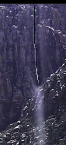
FIGURE 4.30 A Clone stroke covers the top of a lens flare. The flare appears as a vertical white stripe. The stroke is selected, revealing the stroke spline at the top of the figure. A sample script is included as rotopaintclone.nk in the Chapters/Chapter4/Scripts/ directory on the DVD.
You can animate a Clone stroke’s transformations through the Transform tab. The Clone tab, on the other hand, determines the Transform X, Transform Y, Rotate, Scale, and Skew of the sampled background. For example, if you increase the Scale to 2, the background is scaled by 200% before it is sampled for the stroke.
Using Specialized RotoPaint Tools
Aside from the Brush and Clone tools, you can use the Eraser, Blur, Sharpen, Smear, Dodge, and Burn tools to create specialized results. Brief descriptions of each follow.
Eraser “cuts” a stroke-shaped path into other brush strokes. This is achieved by setting the Source menu, in the Stroke tab, to Background. An Eraser stroke can only function if it is at the top of the stroke stack in the Curves section.
Blur utilizes the Bg input pipe color to create a blurred stroke. For the blur to function, the Source menu, in the Stroke tab, must be set to Foreground. The strength of the blur is determined by the Effect parameter in the Stroke tab. You can use the Blur tool to selectively blur a small section of an image (Figure 4.31).

FIGURE 4.31 A Blur tool stroke blurs a background in a confined area. A sample script is included as rotopaintblur.nk in the Chapters/Chapter4/Scripts/ directory on the DVD.
Sharpen functions in a manner similar to the Blur tool. However, the stroke area is sharpened through a process in which contrast is increased. The strength of the sharpen is determined by the Effect parameter in the Stroke tab.
Smear utilizes the Bg input pipe color. However, the pixels are offset in such a manner as to “push” the pixels ahead of the stroke.
Dodge and Burn utilize the Bg input pipe color. However, their blending modes are set automatically to Color-Dodge and Color-Burn. Dodging lightens the pixels and burning darkens the pixels. The Source menu must be set to Foreground for the Dodge and Burn strokes to function.
The FurnaceCore plug-in set includes the F_RigRemoval and F_Wire-Removal nodes. (The plug-ins appear in the Furnace or the Furnace-Core menu, depending on which version of Nuke you are running.) F_RigRemoval attempts to remove a rig (some type of a moving object) from an image sequence or movie and fill the void with the original empty background. Basic steps for its use are as follows:
1. Connect the F_RigRemoval’s Src pipe to the output that carries the rig.
2. Open the F_RigRemoval properties panel. With the Rig Region menu set to Box, interactively place the red rig region box in the Viewer. The box should loosely cover the rig (moving object).
3. Expand the Rig Region Box section in the properties panel and set keys for the Rig Region BL (bottom left) and Rig Region TR (top right) corner values. Move ahead on the timeline and reposition the region box so that it covers the rig at all times.
4. Examine the node’s output. If the rig is not completely removed, you can adjust the Num Frames parameter. Num Frames determines how many frames forward and backward the node will go on the time line to seek data (image pixels without the rig) to fill the void left by the removed rig.
The F_RigRemoval includes a RigMask input pipe, which you can connect to a Roto node or other animated mask. To use the RigMask input, you must change Rig Region from Box to one of the alpha or luminance options.
In contrast, F_WireRemoval is designed to remove wires that may remain from physical stunt or light rigs used on a set. The node’s basic workflow includes the following steps:
1. Connect the output containing the wire to the node’s Source pipe. If a clean plate is available (same camera position without the wire), connect it to the CleanPlate pipe.
2. Identify the wire position by interactively moving the points of the node’s wire widget in the Viewer. If the wire moves over time, activate the node’s built-in wire tracker.
3. Once the wire tracking is successful for all the frames, choose a repair method through the Repair menu. Options include Spatial (current frame only), Spatial With Local Motion (motion estimation using previous and next frame), Spatial With Global Motion (motion estimation for entire sequence), and Clean Plate (if the CleanPlate pipe is connected).
For additional information on motion tracking (which uses controls similar to the F_WireRemoval’s wire tracking), see Chapter 8. For information on motion estimation, see Chapter 6. For more information on the F_RigRemoval and F_WireRemoval nodes, see the “User Guide for Furnace” PDF available at The Foundry’s website (www.thefoundry.co.uk).
Part 4: Adding a Shadow and Rotoscoping a Hand
In Part 3 of this tutorial, we color graded the heart render and background image sequence to create better integration. Part 4 rotoscopes the character so that the heart can sit behind the hand. In addition, a shadow is created by duplicating the heart render output and applying filters to the duplicate.
1. Open the Nuke script you saved after completing Part 3 of this tutorial. A sample Nuke script is included as Tutorial1.3.nk in the Tutorials/Tutorial1/Scripts/ directory on the DVD.
2. Move the time marker to frame 1 so that the heart is at rest on the ground. Open the Transform1 node’s properties panel and temporarily set Motionblur to 0. This will speed up the Viewer as you update the node network.
3. In the Node Graph, RMB-click and select Transform > Transform or press the T key. LMB-drag the input pipe of the new Transform2 node and drop it on top of the Read2 node (see Figure 4.36 at the end of this section). Disconnect the Transform1 node from the Merge1 node. Connect the input A pipe of the Merge1 node to the output of the Transform2 node. Connect the A2 input pipe of the Merge1 node to the output of the Transform1 node. The A2 pipe is drawn as a pipe stub on the left side of the Merge1 node icon. If you cannot see the pipe stub (it may be covered by the A pipe connection), LMB-drag the Transform1 node output pipe and drop it on the Merge1 node. The A connection is relabeled A1 and the new connection between Transform1 and Merge1 is labeled A2. A Merge node can accept two or more connections. This series of connections allows a second iteration of the heart render to be placed over the background image sequence. The output of Transform2 is placed “under” the output of Transform1.
4. Open the Transform2 node’s properties panel. Set Skew to 1, Rotate to – 12, Translate X to –250, and Translate Y to –310. Click the 2 button beside Scale. This reveals the Scale W and Scale H cells. Set W to 0.7 and H to 0.8. This series of changes skews and elongates the heart so that it runs roughly in the same direction as other ground shadows contained in the image sequence.
5. Select the Transform2 node, RMB-click, and choose Color > Grade (or press G). Open the Grade2 node’s properties panel. Change Blackpoint to 1. This turns the skewed heart to pure black (Figure 4.32). In this case, all values in the render equal to or less than 1 are converted to a value of 0.
6. With the Grade2 node selected, RMB-click, and choose Color > Grade (or press G). Open the Grade3 node’s properties panel. Change the Channels menu to Alpha. Change the Gain to 0.68. This decreases the intensity of the whites within the alpha channel. In turn, the heart render (now converted into a shadow) becomes less opaque. With the Grade3 node selected, RMB-click and choose Filter > Blur (or press B). Open the Blur1 node’s properties panel and change Size to 22. This softens the shadow (Figure 4.33).

FIGURE 4.32 A second iteration of the heart render is scaled, rotated, and skewed with a Transform node. The result is darkened with a Grade node to emulate a shadow.
7. Move the time marker to frame 24. This is the last frame that features a static heart. Open the Trasform2 node’s properties panel. Click the Animation Menu button beside Translate and choose Set Key. The X and Y cells turn blue. Move the time marker to frame 27. This is the frame where the heart render is kicked out of sight. With the Transform2 node selected, interactively move the shadow past the top-right corner of the bounding box. A new keyframe is placed on the timeline. This motion allows the shadow to move in correspondence with the heart.

FIGURE 4.33 The shadow is made more transparent by darkening the alpha channel with an additional Grade node. The shadow is softened with a Blur node.
8. Move the time marker to frame 22. This is the first frame where the heart render occludes the character’s hand. To place the heart behind the hand, you will need to rotoscope. With no nodes selected, choose Draw > Roto. Connect the Roto1 node’s Bg input pipe to the Read1 node. Create a new Viewer by choosing Viewer > Create New Viewer from the menu bar (Figure 4.34). Connect the output of the Roto1 node to Viewer2. Switch to the Viewer2 tab in the Viewer pane.
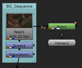
FIGURE 4.34 Initial rotoscope setup.
9. Click the Bezier tool in the Roto node toolbar. Draw a bezier shape by clicking in the Viewer. Close the shape so that it surrounds the fingers and palm. When the shape is closed, it’s filled with white, which obscures the image sequence. Open the Roto1 node’s properties panel and switch to the Shape tab. Change the Source menu to Background. This fills the shape with the original color found in the image sequence, which is connected to the Bg input pipe (Figure 4.35). Adjust the tangents and the feathers of the points (see the “Editing a Bezier and Using B-Splines” section earlier in this chapter for more information). Move the time marker to frame 24 and readjust the shape contour to fit the hand. A new keyframe is laid down. Move the time marker to frame 23 and adjust the shape again.
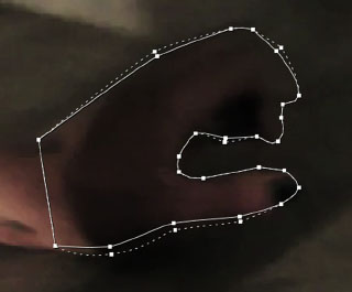
FIGURE 4.35 A bezier shape is drawn around the fingers and palm.
10. Once you’re satisfied with the rotoscoped bezier shape, switch back to the Viewer1 tab. Change the Roto1 node’s Source menu back to Color. Disconnect the Bg pipe from the Read1 node. Connect the output of Roto1 to the Mask input of the Merge1 node (Figure 4.36). This causes the alpha matte of the Roto1 node to affect both the A1 and A2 inputs of the Merge1 node. Hence, a piece of the heart and shadow is cut out in the shape of the fingers. To invert the result, open the Roto1 node’s properties panel, and select the Inverted checkbox beside the Bezier1 curve in the Curves section. The matte is inverted and a hole in the shape of the fingers is cut into the heart and shadow. Thus, the heart and shadow fits “behind” the hand (Figure 4.37). To increase the softness of the alpha matte edge, raise the Roto1 node’s Feather parameter value. To temporarily hide the bezier curve in the Viewer, press O.
This concludes Tutorial 1. Reactivate motion blur by returning the Transform1 node’s Motionblur parameter to 1. Render a test movie by selecting the Merge1 node and choosing Render > Flipbook Selected from the menu bar. As a bonus step, you can refine the transform animation of the heart so that the render matches the slight camera move present in the plate before the kick. (It’s also possible to apply motion tracking to the plate; motion tracking is discussed in Chapter 8.) A sample Nuke script is included as Tutorial1.final.nk in the Tutorials/Tutorial1/Scripts/ directory on the DVD.

FIGURE 4.36 The final node network for Tutorial 1.

FIGURE 4.37 The Bezier shape is used as a Mask input for the Merge1 node, thus cutting a hole into the heart render.
Tutorial 2: Flying a Spaceship
Part 3: Cloaking the Ship with a Procedural Matte
In Part 2 of this tutorial, we color graded the composite to create lighting suitable for a sunset or sunrise. Part 3 mattes the spaceship so that it’s partially transparent (as if it carries a device that allows it to become invisible).
1. Open the Nuke script you saved after completing Part 2 of this tutorial. A sample Nuke script is included as Tutorial2.2.nk in the Tutorials/Tutorial2/Scripts/ directory on the DVD.
2. In the Node Graph, RMB-click and choose Draw > Noise. With the Noise1 node selected, RMB-click and choose Color > Grade. Connect the output of the Grade1 node to the Mask input of the Merge1 node. Create a new Viewer by choosing Viewer > Create New Viewer from the menu bar. Connect Viewer2 to the Grade1 node. Use Figure 4.38 as reference for the final node network.

FIGURE 4.38 The final node network for Tutorial 2.
3. Switch to the Viewer2 tab. The Noise1 node creates a grayscale, procedural noise pattern (Figure 4.39). The same pattern appears in the RGB channels and the alpha channel. (The Noise node, along with other additional filter nodes, are discussed in more detail in Chapter 6.) Switch to the Viewer1 tab. The spaceship becomes partially transparent (Figure 4.40). Thanks to the Mask input, the values carried by the Read1 alpha are multiplied by the values of the Noise1 alpha. Areas of the spaceship render that carry a 0 alpha value remain 0, while areas that carry a 1 alpha value are darkened.

FIGURE 4.39 Pattern created by the Noise1 node.
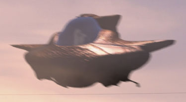
FIGURE 4.40 Partially transparent spaceship, as seen on frame 42.
4. Move the time marker to frame 1. Open the properties panel for the Grade1 node. Change the Channels menu from Rgb to Rgba. Place the mouse over the Lift numeric cell, RMB-click, and choose Set Key from the menu. A keyframe is laid down for the current Lift value, which is 0. (You can set a keyframe for any parameter in this fashion.) Move the time marker to frame 60. Change the Lift value to 1. Switch to the Viewer2 tab. Play back the timeline. Setting two keyframes on the Lift parameter causes the noise pattern to change from its default grayscale to pure white. Switch to the Viewer1 tab. Play back the timeline. The spaceship starts semi-transparent and becomes more opaque as it flies off.
This concludes Tutorial 2. A sample Nuke script is included as Tutorial2.final.nk in the Tutorials/Tutorial2/Scripts/ directory on the DVD. Reactivate motion blur by returning the Transform1 node’s Motionblur parameter to 1. Render a test movie by selecting the HueCorrect1 node and choosing Render > Flip-book Selected from the menu bar. As a bonus step, you can vary the noise pattern over time by keyframing the Z parameter of the Noise1 node.