8

Building Data Models Using Relationships

In the previous chapter, we explored the various data connections that can be made from Tableau Desktop. We will now look at how to combine multiple data sources into a single data model. Tableau has a way of combining data sources at the logical layer through a feature called relationships. This chapter will explore relationships, how to create them, and how they work with different levels of aggregation between tables. This chapter will also explore creating unions between data sources in Tableau Desktop.

In this chapter, we’re going to cover the following topics:

• Using relationships to combine tables at the logical layer
• Understanding the difference between relationships and joins
• Setting performance options for relationships
• Creating unions in Tableau Desktop to add additional rows of data

Note

All the exercises and figures in this chapter will be described by using the Tableau Desktop client software except where noted. You can also recreate all the exercises in this chapter using the Tableau web client, which has a very similar experience to the Desktop client.

Technical requirements

To view the complete list of requirements to run the practical examples in this chapter, please see the Technical requirements section in Chapter 1.

To run the exercises in this chapter, we will need the following files:

• Superstore Sales Orders - US.xlsx
• Product Database.xlsx
• Sales Argentina.csv
• Sales Colombia.csv
• Sales Chile.csv
• Sales Targets.xlsx

If you have not done so already, please download the files, save them to a directory, and make note of the directory name. Create a sub-directory and move the Sales Argentina.csv, Sales Colombia.csv, and Sales Chile.csv files into it.

The files we will be using are all based on the Superstore data, the sample data that Tableau uses in their products.

The files used in the exercises in this chapter can be found at https://github.com/PacktPublishing/Data-Modeling-with-Tableau/.

Using relationships to combine tables at the logical layer

Tableau introduced a new data model in its 2020.2 release called relationships. Up until this release, the only way to expand your analysis to use additional fields from a secondary table in Tableau was to create a join at the physical layer of the data. Relationships offer advantages over physical joins. The advantages come down to quicker and easier data modeling. Just tell Tableau which fields are common between the different tables and let Tableau dynamically generate the right query based on the question asked by the analyst. This means no more pre-aggregation, complex join clauses, and custom SQL queries.

These advantages in modeling lead to two particularly compelling use cases:

• Supporting multiple use cases with a single data model
• Ability to handle different levels of aggregation

Let’s start by exploring multiple use cases with a single data model.

Many use cases with a single data model

We often have a case where an analysis might require two tables to be joined with a left join and another analysis might require a right join (or inner join or outer join). Also, thinking back to Chapter 4, when we joined the sales data with the product data, we had to consider if we wanted to see the following (with sales on the left and products on the right):

• All sales data, even if the product wasn’t in the product database (left join)
• Only sales when a product was in the sales database (inner join)
• All products, even when they weren’t part of a sale (right join)

Each of these leads to viable analyses. To answer all three types of questions in a single Tableau workbook, if you were using joins at the physical level, you would need to create three distinct data models. With relationships, this is not the case. We just let Tableau know that the field that is related between the two tables is Product ID; Tableau handles the rest for us dynamically. We’ll look at each of the preceding three points in detail in the following sections.

All sales data, even if the product wasn’t in the product database (left join)

Let’s use the aggregation of sales targets and the product and sales analyses as examples:

1. Open Tableau Desktop. When you open Tableau Desktop, you will see the Connect pane on the left-hand side of the user interface. From the Connect pane, under the To a File section, select Microsoft Excel. Locate the Superstore Sales Orders - US.xlsx file, select it to highlight it, and click on Open. We should now be looking at the screen shown in Figure 8.1:

Figure 8.1 – Tableau data source page after connecting to US Sales Transactions

2. The Superstore Sales Orders - US.xlsx file has a single sheet called US Sales Transactions, so Tableau automatically added that sheet to our canvas as a single table.
3. The data in the table does not contain product information. To find out which products have sold and which products haven’t sold, we need to create a relationship with our product database. Click on the Add link to the right of Connections. Under the To a File section, select Microsoft Excel. Locate the Product Database.xlsx file, select it to highlight it, and click on Open.

Our screen should now look like Figure 8.2. We now have two data sources in our workbook, namely Superstore Sales Orders – US and Product Database. The Product Database.xlsx file also only has a single sheet. This sheet is called Product DB:

Figure 8.2 – Data source page with Product DB added

4. To create our first relationship, drag the Product DB sheet onto the canvas. You should see a flexible line as you drag it to the canvas, as seen in Figure 8.3. This line is called a noodle and represents a relationship. Release the mouse button to form the relationship:

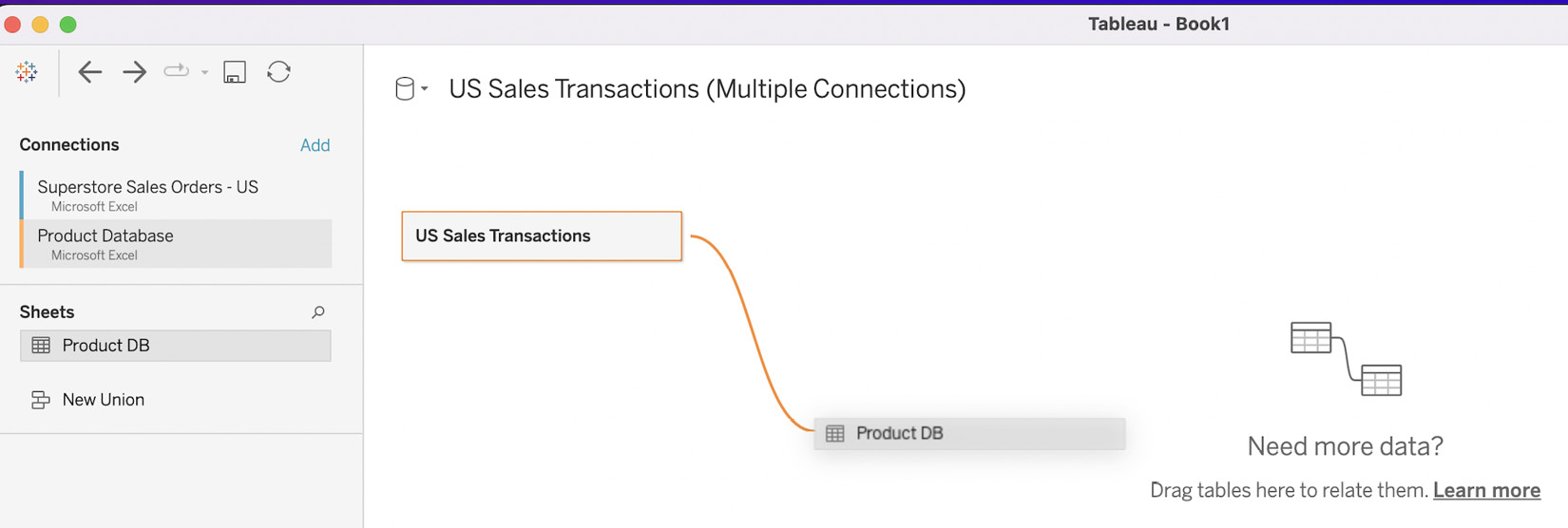
Figure 8.3 – Product DB with a noodle connection to US Sales Transactions

5. To finish our relationship, click on the noodle line that connects the two tables and notice the area of the screen to the left of the data details pane, as seen in Figure 8.4:

Figure 8.4 – Configuring the relationship fields

6. The first thing we see is the area to instruct Tableau on how these tables relate to each other. Tableau picked up that there is a field named Product ID in both tables, so it creates that as a default. We will leave this default as it is correct for our use case. It is always good to check these fields, even when it looks like Tableau has found the right field. There are cases when the same field in two tables contains slightly different information. Notice that we could change these fields, add additional fields, and use operators other than =.
7. The next section can be expanded to show Performance Options. Two options can be set here: Cardinality and Referential Integrity. We are going to look at how to optimize performance later in this chapter. For now, we are going to leave the default setting as-is in our example.
8. Now, let’s see how Tableau creates dynamic joins, depending on the question we want to ask. For our first question, let’s see how we answer the question of, “which products have we sold the most?” Click on Sheet 1 to begin. Let’s look at our data pane to see how Tableau has arranged the metadata in our data model, as seen in Figure 8.5:

Figure 8.5 – The data pane after creating a relationship

9. The first thing we notice is that Tableau organizes our data by source table. Toward the top of the data pane, we see all the fields from the Product DB table in a collapsible list. The discrete fields from the table show up at the top of the list, sorted alphabetically, with a line that separates the continuous fields, which are also sorted alphabetically. This process repeats itself for all tables; in our case, the only other table is US Sales Transactions. If we collapse these tables, we will see the fields that Tableau automatically generates, and could also be used across tables. These are listed at the bottom of the data pane, as seen in Figure 8.6:

Figure 8.6 – Fields generated by Tableau

10. With an understanding of our data, let’s look at the answer to our question regarding products that have sold the most. Under the US Sales Transactions table, double-click Sales to bring it into the view. Under the Product DB table, double-click to bring Product Name into the view. Your screen should now look like what’s shown in Figure 8.7:

Figure 8.7 – Sales by Product Name

11. To make it easier to get to our answer of the product that sold the most, click on the Swap Rows and Columns icon in the toolbar below the menu bar, as seen in Figure 8.8:

Figure 8.8 – The Tableau Desktop toolbar

Click on the Sort Descending button, which is two icons to the right of the Swaps Rows and Columns icon. You should now have a view that looks like Figure 8.9:

Figure 8.9 – Product names that have sold the most sorted descending

12. We notice two interesting pieces of information right away. The first is that we have a lot of sales where there is no product name attached to them. The second is that we have 1789 null records as well, which we can see if we hover over the >2K nulls icon at the bottom-right corner of the canvas, as seen in Figure 8.10:

Figure 8.10 – Hovering over the nulls indicator

13. First, let’s look at all the sales where Product Name has a Null value. We told Tableau to create a relationship between these tables based on Product ID, so let’s bring that into our view. Drag the Product ID (Product DB) field from the Product DB table and the Product ID field from the US Sales Transactions table onto the Rows shelf in the view. The result should look like what’s shown in Figure 8.11. Leave Tableau Desktop open at this point. We will continue from this point in the next section:

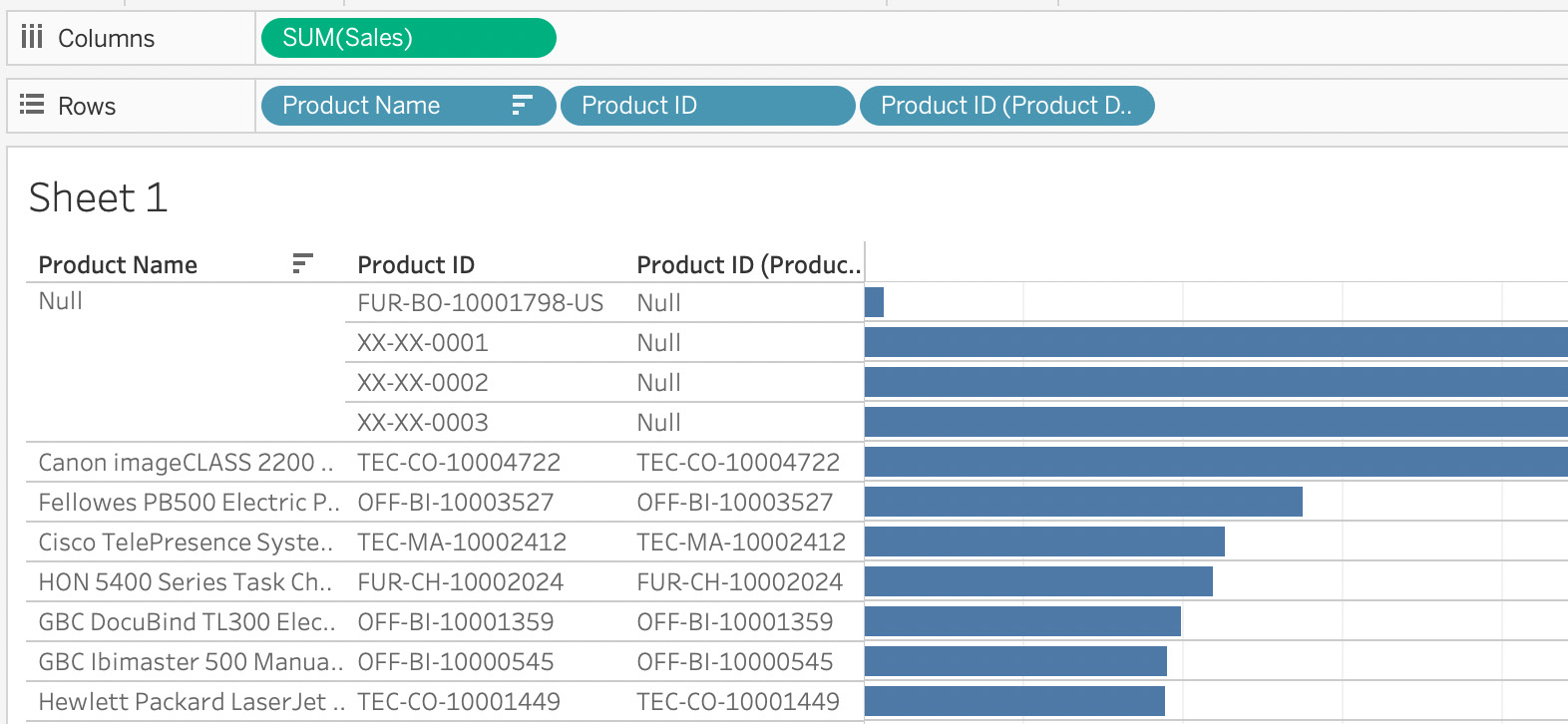
Figure 8.11 – Uncovering null product names

Now that we have the answer to our question of all sales, even if they do not have a Product ID associated with them, let’s look at sales when there is only a Product ID on the sales record.

Only sales when a product was in the sales database (inner join)

Let’s begin:

1. We can see that there are two product IDs in the sales transactions that are not in our product database. Looking back to Chapter 4, we have already seen these and discovered how to clean and filter values like these in our data model. Right-click on the Null cell under Product Name and select Exclude to filter out these values, as seen in Figure 8.12:

Figure 8.12 – Exclude null values

2. We now have the answer to our question. Canon imageCLASS 2200 Advanced Copier is our top-selling product with sales of $61,600. If we look at the Filters shelf, we will see the Product Name filter. Right-click on the Product Name filter in the Filters shelf and select Edit Filter, as seen in Figure 8.13:

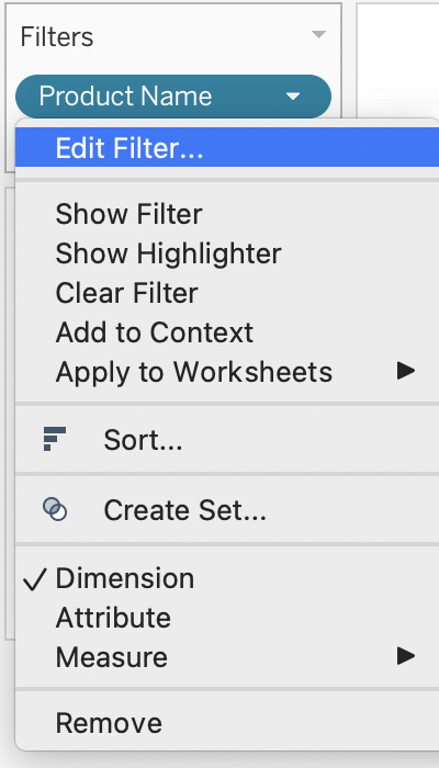
Figure 8.13 – Edit Filter…

3. The result of our filter will come up as per Figure 8.14:

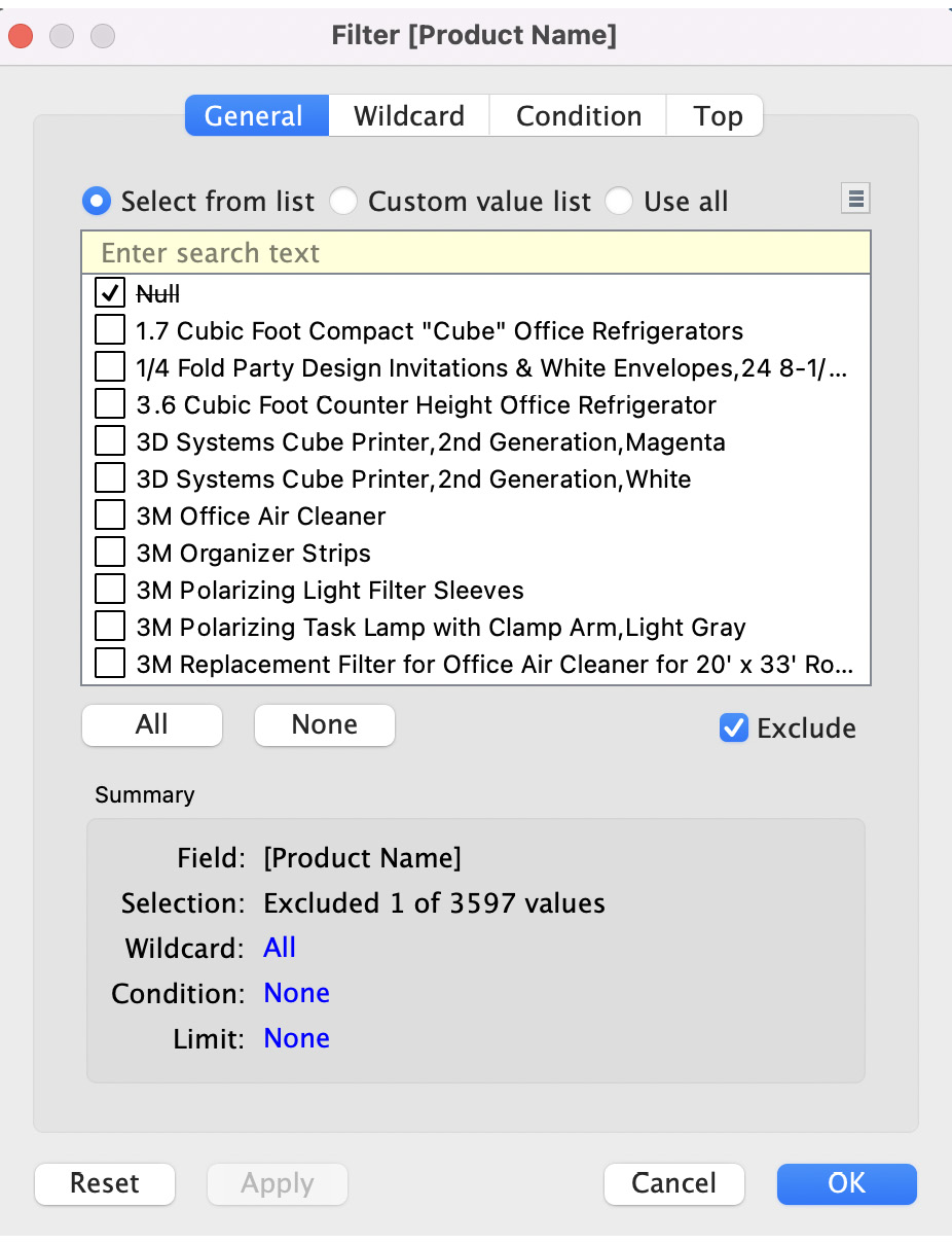
Figure 8.14 – Filter excluding nulls

Tableau created an exclude filter on null values based on the exclude gesture we made in Step 15. This filter is currently only applied in the analysis we are doing in Sheet 1. We could add a data source filter, as we explored in Chapter 7. Additionally, we can apply this filter to more than one sheet. Right-click on the filter and select Apply to Worksheets | All Using This Data Source, as seen in Figure 8.15. This is another way to create a data source filter. Leave Tableau Desktop open at this point. We will pick up from this step in the next section:

Figure 8.15 – Filtering to all using this data source

Now that we have the answer to the question of which product we have sold the most, let’s answer the question, “what percentage of all products in our catalog have not sold?”

All products even when they weren’t part of a sale (right join)

Let’s find out what percentage of all products in our catalog have not sold:

1. To quickly see how many Product ID records are in each table, let’s start by creating two new sheets. Click on the icon to the right of Sheet 1 near the bottom left of the screen, as seen in Figure 8.16, to create a new sheet, which will be labeled Sheet 2. Repeat this to create Sheet 3 as well:

Figure 8.16 – Creating a new sheet

2. Go to Sheet 2. Double-click on the Product ID field under the US Sales Transaction table. This will create a list of all the Product IDs that have sold. We know this because they are coming from the sales table. If you look at the bottom left of the screen, you will notice there are 1861 marks, as per Figure 8.17. This means there are 1,861 products sold in our database table. If you click back on Sheet 1, you will notice the same number of records, as expected. To get these records, Tableau only had to query the US Sales Transaction table without creating a join to the Product DB table:

Figure 8.17 – 1,861 sold products

3. Go to Sheet 3. This time, double-click on the Product ID (Product DB) field under the Product DB table. You will now see 10292 marks. This means there are 10,292 total products in our product database. To get these records, Tableau only had to query the Product DB table without creating a join to the US Sales Transaction table. In other words, we have sold 1,861 products at least once while 8,431 products have never been sold. Let’s validate these numbers to be sure.
4. There are several ways to see which products have and have not sold in the same view. Before starting, click to create a new sheet, Sheet 4. For this exercise, let’s do it using a set. Sets are specialized fields that define a subset of data based on the conditions you define. Go to the newly created Sheet 4. Right-click on the Product ID (Product DB) field and select Create | Set, as per Figure 8.18:

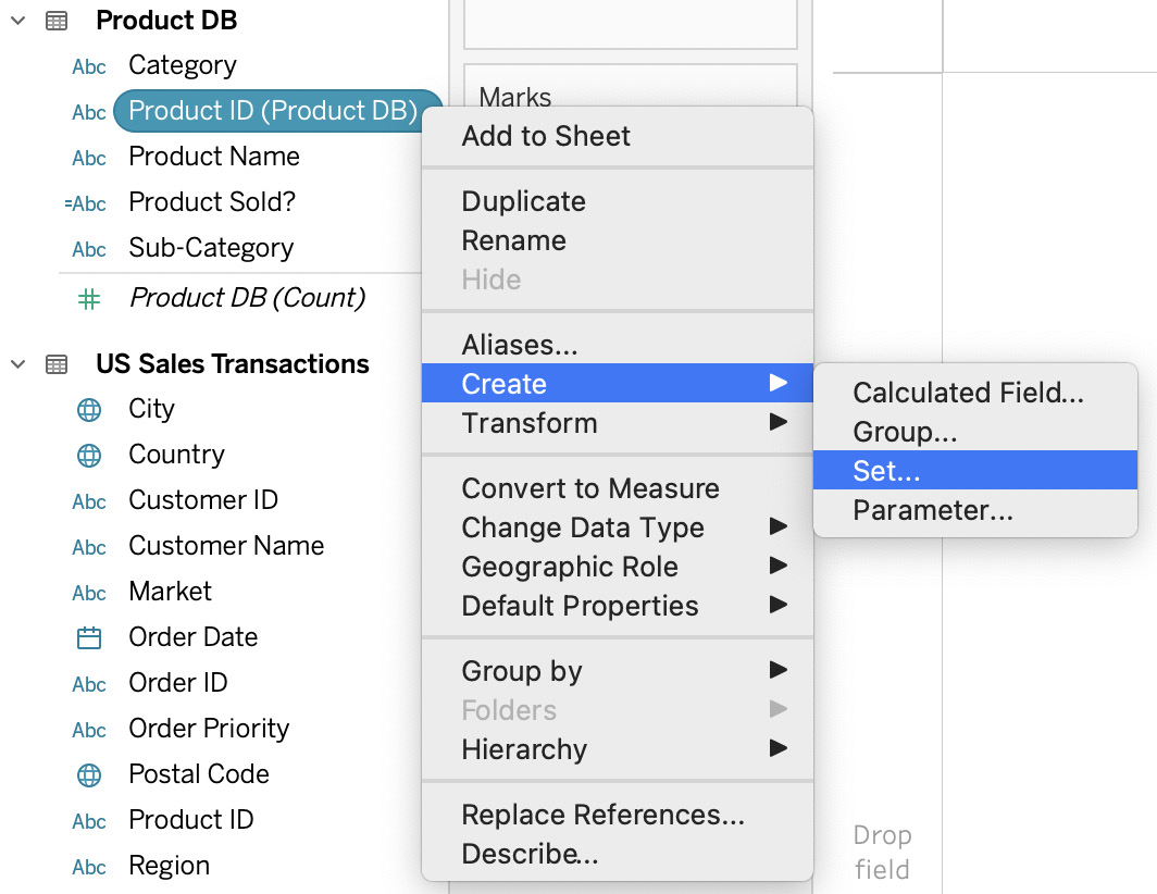
Figure 8.18 – Creating a set from Product ID (Product DB)

5. Click on the Condition tab and select By field. Select Sales as the field, Sum as the aggregation, and then > as the operator and 0 as the value, as seen in Figure 8.19. This will create a new set with Product IDs that sold IN the set and those with no sales OUT of the set. Press OK to finish creating the set:

Figure 8.19 – Create Set

6. To get the percentage of products from our product database that have not sold, drag the new Product ID (Product DB) Set field to the Rows shelf. You should now see In and Out, as seen in Figure 8.20:

Figure 8.20 – Product ID set on the view

7. Drag the Product ID (Product DB) field to the Text card. Right-click on Product ID (Product DB) in the Marks card and select Measure | Count (Distinct), as seen in Figure 8.21. This will give us a count of unique Product IDs that have sold (IN) and have not sold (OUT):

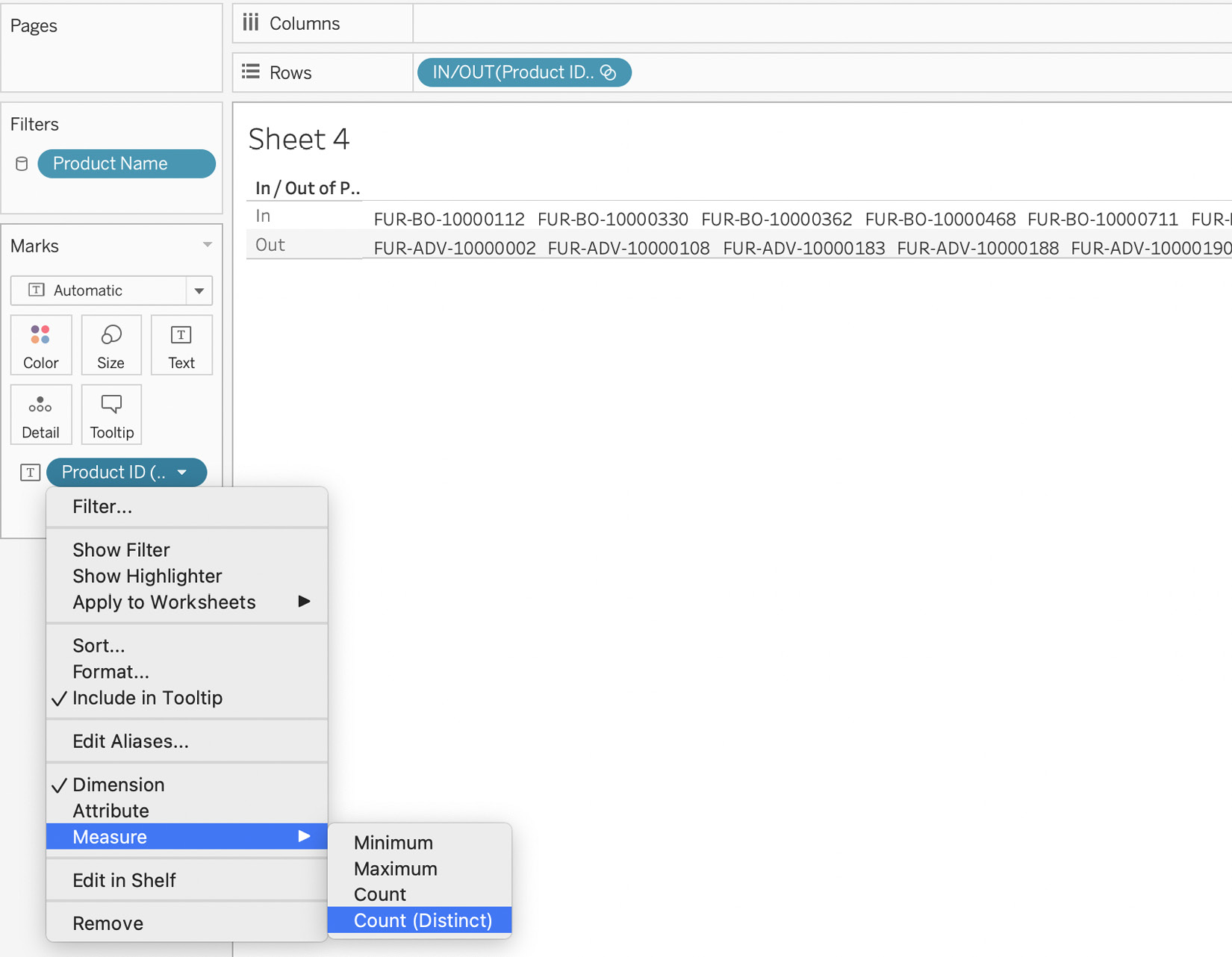
Figure 8.21 – Products that have sold and not sold

8. As a final step, right-click on CNTD(Product ID (Product DB)) in the Marks card and select Quick Table Calculation | Percent of Total, as seen in Figure 8.22:

Figure 8.22 – Percent of Total

9. This will give us our answer that 81.92% of the products in our product database have not been sold, as per Figure 8.23. This is the first query that we have looked at where Tableau needed to query both tables. Tableau has handled all of our queries and joins for us dynamically:

Figure 8.23 – Our answer!

Now that we have explored how to support multiple use cases with a single data model using relationships, let’s move on to creating relationships when the tables are at different levels of aggregation.

Ability to handle tables at different levels of aggregation

When you join two tables together, Tableau will flatten the results into a single table. This means that all data needs to be at the same level of detail. With relationships, Tableau will know which table your field is in and will be able to handle it at the right level of detail. Looking back to Chapter 4, we had to aggregate our sales data source before we could join it to the monthly sales target in Tableau Prep Builder. We do not have to do this with relationships. We will now create a relationship between two tables at different levels of aggregation:

1. Open Tableau Desktop. From the Connect pane, under the To a File section, select Microsoft Excel. Locate the Sales Targets.xlsx file, select it to highlight it, and click on Open. This workbook has a single sheet with sales targets for 12 months for five countries in 2014.
2. We need to pivot our data before we can create a relationship with our sales transactions. Click on the 1/1/2014 field, hold down the Shift key, scroll to the right until you get to the end, and click on the 12/1/2014 field while still holding down Shift. Right-click on the 12/1/2014 field to bring up the ▼ and select Pivot, as seen in Figure 8.24:

Figure 8.24 – First pivot date fields

3. After the pivot, rename Pivot Field Names to Date and change the field type to Date. Rename Pivot Field Values to Sales Targets. The result is seen in Figure 8.25:

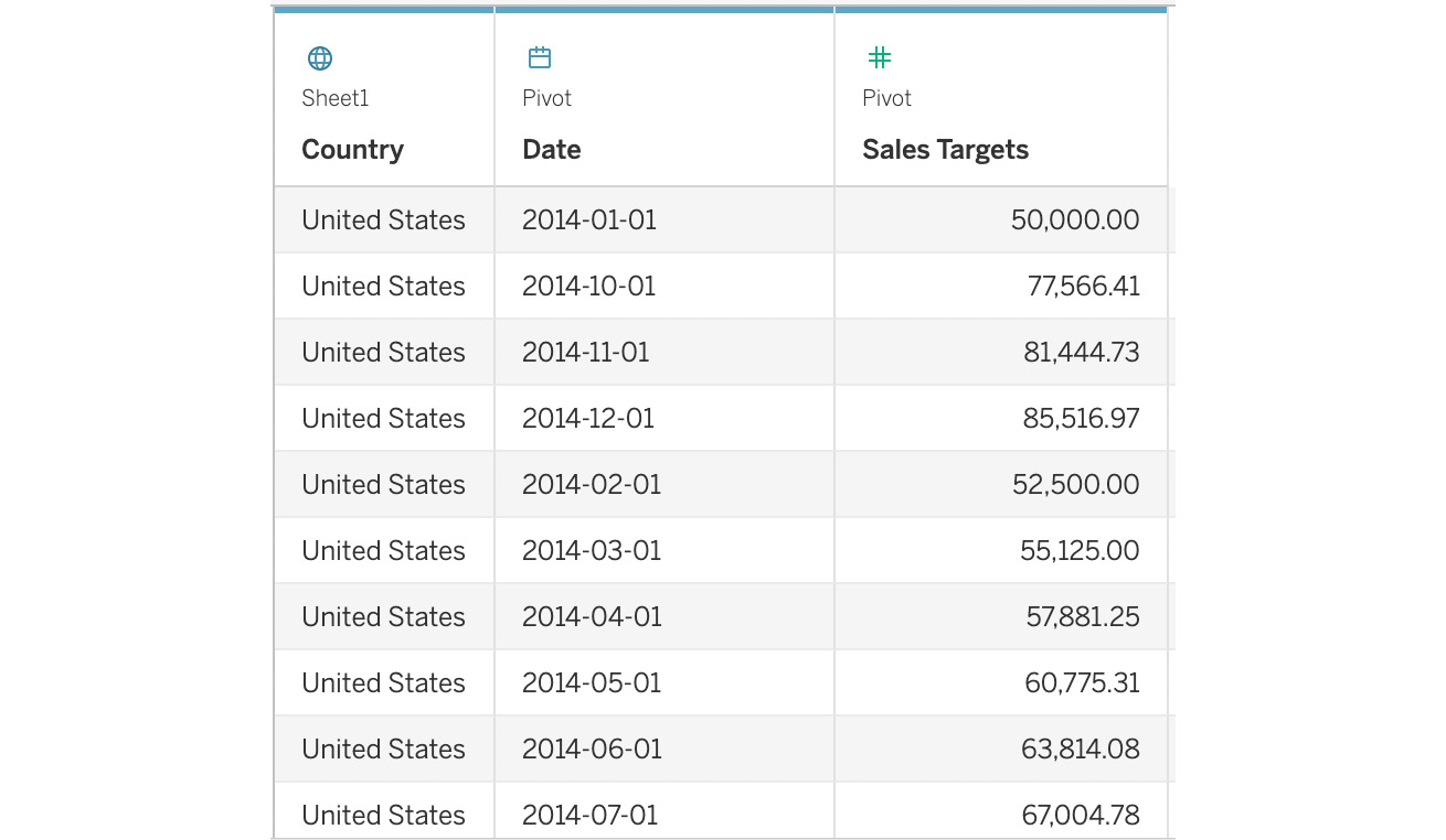
Figure 8.25 – Renaming and changing the field type after the pivot

4. We can create a relationship with our sales data now that our sales targets are in the spreadsheet table format that works with Tableau. Click on the Add link to the right of Connections. Under the To a File section, select Microsoft Excel. Locate the Superstore Sales Orders - US.xlsx file, select it to highlight it, and click on Open.
5. Drag the US Sales Transactions sheet onto the canvas until the noodle appears. Release the left mouse button to drop the sheet onto the canvas and create a relationship, as seen in Figure 8.26:

Figure 8.26 – Relationship between sales targets and US Sales Transactions

6. We can see that Tableau thinks the relationship should be made on Country. This is partially true, but we also want to make sure that Tableau knows the relationship also occurs based on date. Under How do relationships differ from joins?, click on Add more fields, as seen in Figure 8.27:

Figure 8.27 – Relationship field mapping

7. On the Sheet1 side, add Date. Keep the operator as = and select Create Relationship Calculation..., from under the US Sales Transactions side as seen in Figure 8.28. We need to create a relationship calculation because we do not want the sales targets to line up with the first sales date of the month. We need the sales targets to line up with monthly sales:

Figure 8.28 – Create Relationship Calculation…

8. The relationship calculation we are going to create has the syntax of DATE(DATETRUNC('month', [Order Date])). Enter this in the calculation dialog and press OK, as per Figure 8.29:

Figure 8.29 – Relationship calculation

The reason for this calculation is we want all the sales for the month to map to the first day of the month as this is the way the monthly data is represented in the sales target table. The reason the calculation is wrapped in the DATE function is that Tableau will always make a DATETRUNC calculation of the Date/Time type, which would be a mismatch to Date in the sales targets sheet.

9. To see how the relationship handled the difference in both levels of detail and having five countries when our sales data only had one country, click on Sheet 1. Drag and drop the Date field from the Sheet1 table to Columns. Right-click on the YEAR(Date) pill on the Columns shelf and change the aggregation to the top Month option, as seen in Figure 8.30:

Figure 8.30 – Dragging Date to Columns

10. From the Sheet1 table, drag and drop Country to the Rows shelf and drag and drop Sales Targets to the Text marks card. The result is shown in Figure 8.31:

Figure 8.31 – Sales targets by county and month

11. Drag and drop Country from the Sheet1 table to the Filters shelf and select only United States. Drag and drop Date from the Sheet1 table to Filters, choose Year, and select only 2014 (the only available option). To see what percentage of the sales target has been achieved, we can create a field called % Sales Target. Click on the ▼ icon to the right of the search box and select Create Calculated Field…. Then, enter SUM([Sales])/SUM([Sales Targets]) in the dialog box, as seen in Figure 8.32:

Figure 8.32 – % Sales Target achieved calculation

12. You will notice that the calculation falls in the data pane outside the area of either of the tables. The reason for this is to signify that Tableau needs to query both tables to create the calculation. Before adding this calculation to our view, right-click on the % Sales Target field, select Default Properties | Number Format…, as shown in Figure 8.33, and then pick a percentage with 2 decimal places:

Figure 8.33 – Change number format

13. To complete our analysis, drag and drop the new % Sales Target on top of the Sales Target field in the Marks card to replace it in the view, as seen in Figure 8.34. The result is the answer to the question “what percentage of the sales target was achieved in the US per month?” and we answered it without needing to aggregate our sales transactions first:

Figure 8.34 – Sales targets achieved per month

In this section, we looked at using relationships to deal with tables at different levels of aggregation. This saves a lot of time and complexity in data modeling. It also saves a lot of time in creating fewer data models and the need for less quality assurance by avoiding complicated joins.

In the next section, we will explore how relationships are different than joins.

Understanding the differences between relationships and joins

It was a straightforward path to answering our question of which product had the highest sales using a relationship. If we had used a join, we could have made a left join with the US Sales Transactions table on the left and the Product DB table on the right and gotten the same answer. However, if we had created that join, it would have excluded all the products that did not sell from the product database, so we may not have been able to answer our question about the percentage of products that did not sell. We could have answered this question with a right join but then we wouldn’t have been able to find the incorrect product IDs because they would not have been identified in our join. We could have created a full outer join, but this would have resulted in a lot of null values in our data, which would make analysis more difficult and caused an explosion of our data.

These limitations make relationships such a great choice. We just let Tableau know which field(s) are common across the tables and let Tableau handle the right queries and join types.

We will take a deeper dive into joins in Chapter 9, including use cases for joins over relationships.

Setting performance options for relationships

In the previous two sections, we looked at relationships and how they differ from joins. As relationships are dynamic, they can sometimes create queries that could be better optimized by telling Tableau more about our data.

Performance Options is available in the user interface under the field mappings, as seen in Figure 8.35:

Figure 8.35 – Performance options

In most cases, the best practice is to leave the default options as-is unless we are 100% sure of our data. Let’s look at these two settings and why the default is best:

• Cardinality: You can effectively use this to tell Tableau when a field is a unique key/index field. Using our example of product sales and the product catalog where product sales are on the left, we would want to leave Many on the left-hand side because a Product ID could be sold many times. If we were 100% sure we had no duplicates in our data – exactly one row per Product ID – we could set the right-hand side to One. Unless we are confident this is true, it is better to leave Many as-is; otherwise, there could be duplicate aggregate values in views created from the data model.
• Referential Integrity: Changing this from Some records match to All records match can speed up performance, but again only if you are confident. In our products example again, it seems like we should be able to have All records match on the left and Some records match on the right because only 80% or so of the records in the product database have a match in sales, but every record in the sales transactions should have a matching Product ID in the product database. If you remember, this wasn’t true as we had one bad Product ID, along with a few records with a null Product ID. While setting the product database side to All records match would have resulted in more simple queries (which means faster queries in big data tables), we would have missed those records and might have ended up with confusing results.

In this section, we looked at optimizing the queries Tableau generates from relationships. We also learned how to change the default settings when we know exactly what is in our data to ensure we don’t end up with confusing result sets in our analysis.

So far, we have looked at adding additional fields to our data model by using relationships. In the next section, we will explore the use of unions to add additional rows of data in Tableau Desktop.

Creating manual and wildcard unions in Tableau Desktop to add additional rows of data

We use relationships to add additional fields to our data. For cases where we need to add additional rows from other tables or files, we use unions. We can union new data via manual union or wildcard union. We will look at both methods in the upcoming sections.

It is important to note that Tableau Desktop can create relationships and joins between tables, regardless of whether they are in the same database or across multiple databases (if the database supports cross-database joins). However, unions can only be created by tables in the same database. In the case of Microsoft Excel, this would mean the unions of multiple sheets within the same Excel workbook but not the ability to union across different workbooks.

Tableau Desktop can create unions across multiple text files. It is a common use case to get data dumps in the form of delimited files, which can then be joined together in Tableau Desktop. In our example, we will be using sample data representing Superstore sales from three South American countries, with each country represented in a unique file.

Manual union

We perform a manual union by dragging an addition table to an existing connection on the canvas of the data source page. We will start with a union of Chile Sales data to Argentina Sales. Before we begin, make sure you have the following files copied from GitHub into the same folder on your computer:

• Sales Argentina.csv
• Sales Colombia.csv
• Sales Chile.csv

It will make your union easier if these three files are in a directory with no other files, although this isn’t required. The reason is that the easiest and most manageable method of creating a union of text files is by having all those files and no other files in the same directory. As each of the files acts as a table, we will be using the terms files and tables interchangeably during this exercise:

1. Open Tableau Desktop. From the Connect pane, under the To a File section, select Text file. Locate the Sales Argentina.csv file, select it to highlight it, and click on Open. We should now be looking at a screen similar to the one shown in Figure 8.36:

Figure 8.36 – Tableau data source page after connecting to the Sales Argentina.csv file

2. The easiest way to create a manual union is to take the table you want to union and drag it under the first table on the canvas. Put your mouse over Sales Chile.csv in the left pane, hold down the left mouse button, and drag the table under the Sales Argentina.csv card onto the canvas until the Union drop area appears, as shown in Figure 8.37:

Figure 8.37 – Union drop zone

Tableau will show you a noodle, as per the relationships exercises from earlier in this chapter, until you find the Union drop zone. Release the left mouse button when you are over the Union drop zone.

3. We will know if the union worked when the union icon of stacked building blocks appears in front of the Sales Argentina.csv card on the canvas, as seen in Figure 8.38:

Figure 8.38 – Union icon in front of Sales Argentina.csv

4. To check the results of our union, you can hover to the right of the card with Sales Argentina.csv until the ▼ icon shows. Click on the down arrow to bring up the menu and select Edit Union…, as seen in Figure 8.39.

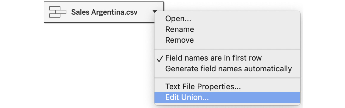
Figure 8.39 – Edit Union…

It is also worth noting that if you have a hard time finding the Union drop area, you can use this same menu to create a new union. If there isn’t a previous union, the menu will say Convert to Union, which will bring up the union dialog box that we can see in the next step.

5. We can now see the two tables that make up our union in the union dialog box, as seen in Figure 8.40:

Figure 8.40 – Union dialog box

6. We want to add Sales Colombia.csv to our union as well. We can do this in one of two ways. The first method is by dragging and dropping the Sales Columbia.csv table below Sales Chile.csv in the union dialog, as per Figure 8.41. Do not press OK here as we are going to look at the second method in the next step:

Figure 8.41 – Adding a union manually through drag and drop

7. The other method is through a wildcard union. Click on the Wildcard (automatic) tab in the union dialog box. The result should look like what’s shown in Figure 8.42:

Figure 8.42 – Wildcard union

8. A wildcard union is a great option when you have a lot of files, especially if you are regularly getting new files. If the new files match the pattern you set in this dialog, Tableau will automatically add them to your union as they get added to the directory. The options in a wildcard union are as follows:
   • Files: Either include or exclude and then enter a pattern. For example, if you only want files with 2022 in the filename, you could leave Include and enter *2022* as a pattern. Tableau would ignore all the files in the directory or directories except those with 2022 in their filename.
   • Expand search to subfolder: This will tell Tableau to search in the folders below this one in the directory structure.
   • Expand search to parent folder: This will tell Tableau to look in the directory immediately above this directory.
9. Leaving all these options blank tells Tableau to take all the files in the chosen directory, which is determined by the first file we added. If you have the three South American sales files in the same directory with nothing else in the directory, you can press OK now and Tableau will create a data model with these three files in a single union.

We can check to see if our wildcard union worked by clicking on Sheet 1 and then double-clicking on the Country field in the data pane. The result should look like what’s shown in Figure 8.43. We can see a dot for each of the countries from the three files of our union:

Figure 8.43 – Map showing a dot for each country in our union

If we replace our files with new data but keep the same filename, Tableau will automatically pull in the new data. For instance, if new data becomes available for Argentina and a new file overwrites our existing file for Argentina, Tableau will bring in the new data the next time you run the union without any manual intervention.

In this final section of this chapter, we learned about adding new rows of data to our data model through the use of manual and wildcard unions.

Summary

In this chapter, we learned about adding additional fields to our data model through the relationship feature in Tableau. Relationships give us flexibility by allowing us to create relationships at the logical layer of databases. With relationships, we leave the mapping of joining data at the physical layer for Tableau to create dynamically, depending on the field we use in our analyses.

We looked at how relationships are different than joins and various use cases for relationships where joins would result in multiple data models. We also looked at how performance options are available to optimize relationship query performance.

In the final section, we looked at adding additional rows to our data model by using manual and wildcard unions.

The next chapter will focus on creating joins in Tableau Desktop at the physical database layer. We will also explore geospatial joins and custom SQL.