7

Connecting to Data in Tableau Desktop

The two primary tools for connecting to data in Tableau are Tableau Prep Builder and Tableau Desktop. Building off the previous four chapters, which covered Tableau Prep Builder, this chapter focuses on connecting to data in Tableau Desktop.

Tableau Desktop has connectors to many different data sources. These broadly fall into the categories of flat files, database servers, data from the web, and Tableau data servers, called published data sources.

In this chapter, we’re going to check out how to connect to each of these data sources through the following main topics:

• Connecting to files in Tableau Desktop
• The data interpreter feature and pivoting columns to rows
• Connecting to data servers – on-premises, cloud, applications, and file shares
• Web data connectors and additional connectors
• Connecting to data sources that aren’t listed
• Connecting to Tableau published data sources

Note

All the exercises and images in this chapter will be described using the Tableau Desktop client software except where noted. Additionally, you can recreate all the exercises in this chapter using the Tableau web client, which has a very similar experience to the Desktop client.

Technical requirements

To view the complete list of requirements needed to run the practical examples in this chapter, please view the Technical requirements section of Chapter 1.

To run the exercises in this chapter, we will need the following downloaded files:

• GrainDemandProduction.xlsx
• Contribution_Amounts_for_Fiscal_Years_2002-03_to_2015-16.csv
• DETROIT_BIKE_LANES.geojson
• unece.json
• hcilicensed-daycare-center760narrative11-13-15.pdf
• SIPRI-Milex-data-1949-2021.xlsx

Most of the files we are using in this chapter come from data.gov, which has over 300,000 data files that are free to use and offer a wide range of file types and examples.

The SIPRI-Milex-data-1949-2021.xlsx file is associated with a Tableau community project, Makeover Monday, from week 35 of 2022. The file was generated SIPRI Military Expenditure Database. Makeover Monday, found at https://www.makeovermonday.co.uk, is also a great source of data to practice your Tableau skills.

The unece.json file comes from the United Nations Economic Commission for Europe (UNECE).

The files used in the exercises in this chapter can be found at https://github.com/PacktPublishing/Data-Modeling-with-Tableau/.

Connecting to files in Tableau Desktop

Tableau Desktop has the flexibility to connect to many different types of data sources. First, we are going to look at flat files. Flat files have a lot of use cases from the personal analysis of downloaded files to prototyping development before connecting to enterprise databases.

The different types of flat files that Tableau can connect to include the following:

• Microsoft Excel
• Text files (including delimited and character-separated files)
• Spatial files (including Esri, GeoJSON, KML, KMZ, MapInfo, and TopoJSON files)
• Statistical files (including SAS, SPSS, and R output)
• JSON files (JavaScript Object Notation files)
• PDF files (tables from Adobe’s Portable Document Format files)

We will begin by connecting to a Microsoft Excel file.

Getting data from Microsoft Excel files

Microsoft Excel has become an almost ubiquitous method of collecting and analyzing data. Compared with Tableau, Microsoft Excel has very limited visual analytics capabilities and limits on the amount of data that can be analyzed. In cases where the data might only exist in Microsoft Excel, it often makes sense to take that data and extend it with other data in a Tableau data model to provide a rich analysis experience. We will be looking at combining Excel data with other data sources in Chapter 8 and Chapter 9. For now, we will look at bringing Excel files into Tableau.

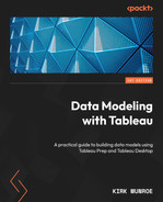
Before we begin this exercise, locate the GrainDemandProduction.xlsx file from the location you saved it in on your computer. Open the file in Microsoft Excel (or another program of choice that will open an xlsx file) and notice the spreadsheet table format, as shown in Figure 7.1:

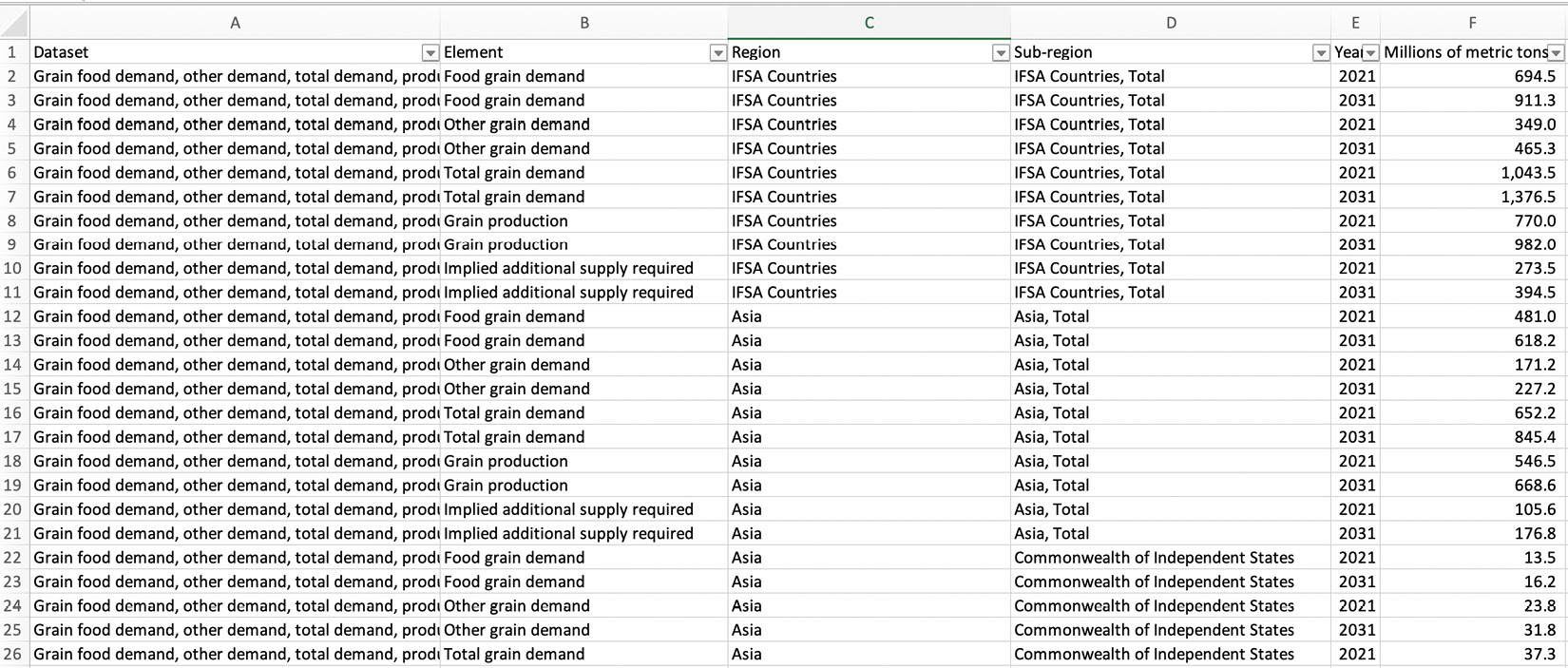
Figure 7.1 – Grain Demand Production table

Let’s bring the Excel file into Tableau:

1. Open Tableau Desktop. When you open Tableau Desktop, you will see the Connect pane on the left-hand side of the user interface, as shown in Figure 7.2:

Figure 7.2 – The Connect pane in Tableau Desktop

2. From the Connect pane, under the To a File section, select Microsoft Excel. Locate the GrainDemandProduction.xlsx file, select it to highlight it, and click on Open.
3. The Tableau Desktop user interface will now take you to the data source page, as shown in Figure 7.3:

Figure 7.3 – Data source page in Tableau Desktop

4. In the bottom-right section of the data source page, there are two grids. The left-hand grid is the metadata grid. This grid is shown in Figure 7.4. You can use the metadata grid to quickly see all the fields in your data model. You can see that Tableau automatically generated a field name for each of the columns in the Microsoft Excel sheet:

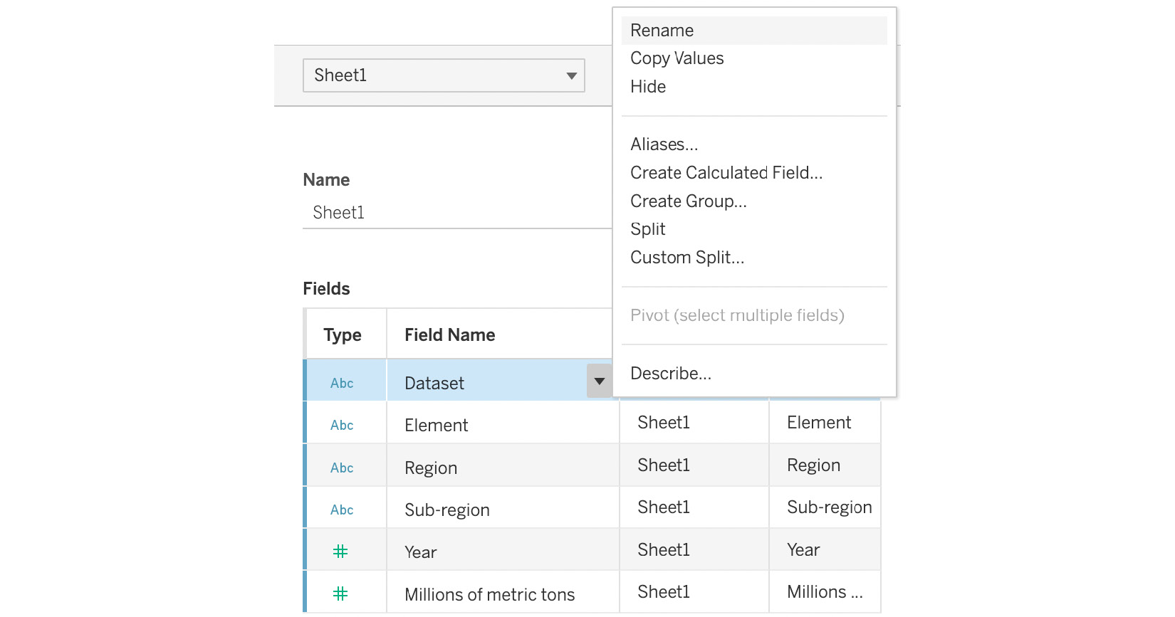
Figure 7.4 – The metadata grid

In the metadata grid, by clicking on the ▼ icon next to the Dataset field name, you can change the table name, field types, and field names. You can hide fields and create calculated fields, split fields, create groups, describe fields, and pivot data. Hiding fields will remove the field from our data model. In the cases of extracts, this means that Tableau will filter the column out of the data it imports. We will look at calculated fields, split fields, describing fields, and groups in Chapter 10. We will be looking at pivots later in this chapter when we look at the data interpreter feature. In our example, the spreadsheet table format imported metadata the way we want it, so we don’t have to make any changes.

5. The bottom-right section contains the data grid as shown in Figure 7.5. This allows us to preview the data in our model. Additionally, we can also perform all the same functions in the data grid that we could in the metadata grid. The advantage of performing these functions in the metadata grid is that we can see more fields on a single screen. The advantage of performing the functions in the data grid is that we can see the impact of our changes on the underlying data model immediately:

Figure 7.5 – The data grid

6. The top and right sections contain the canvas. We will be looking at the canvas in detail in Chapter 8 and Chapter 9. For now, we will look at only the top rightmost section of the canvas where we see the radio button to choose between a Live or Extract connection and the ability to Add filters, as shown in Figure 7.6:

Figure 7.6 – The Live and Extract Add filters

We will be exploring the pros and cons of live connections versus extracts in Chapter 10. For now, it is a good practice to always extract data when working with files. Click on the Extract radio button to create an extract now. After clicking on Extract, you will notice that the Edit and Refresh links now also appear but nothing else appears to happen. We will look at these in the next step.

7. To create our extract, click on Sheet 1 in the bottom-left corner of Tableau Desktop. Now, Tableau will launch a dialog box that prompts you to name and save your extract as seen in Figure 7.7. Give your extract a name and location and press the Save button. For now, feel free to use the default name and location:

Figure 7.7 – The Tableau extract dialog

8. Tableau will now extract your data into a Tableau Hyper file. Hyper is Tableau’s high-performance database for analytical queries from Tableau. We will explore Hyper in more detail in Chapter 10.
9. Now, we will add a filter to limit the number of rows in our data. Click on the Data Source tab in the bottom-left corner of the screen to go back to the data source page. Looking at the upper-right corner of the canvas, where we just created our extract, you will see three options (as shown in Figure 7.6 after step 6 in this section):
   • Edit – This option allows you to control the data in your extract, including adding filters to limit the number of rows and hiding unused filters to limit the number of columns imported to the extract.
   • Refresh – Clicking on this will manually load new data into your extract if it has been added to your source data.
   • Add – This option allows you to add a data source filter that filters data coming from your data source.

It is important to understand the difference between extract and data source filters. In the case of live connections, it is straightforward: data source filters will filter your queries by eliminating filtered data from any analysis in Tableau while extracts filters and the refresh option are not visible as there is no extract. In the case of extracted data, the extract filters are performed before the data source filters. This means that the extract filter will filter out any data that goes into the extract. Then, the data source filter will further filter out any data in the extract and eliminate that data from any analysis in Tableau.

10. In our case, we have extracted data from Excel, so let’s look at the Edit option. Click on Edit and you should see a dialog like the one in Figure 7.8. For now, we are only looking at the filters section. We will look at the other options in Chapter 10 after learning about logical tables in Chapter 8 and physical tables in Chapter 9. Click on the Add button to bring up the filter dialog box:

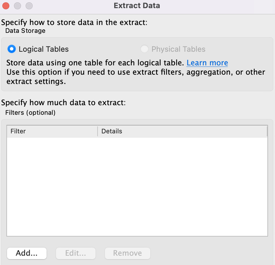
Figure 7.8 – The Extract dialog box

11. Now we can add our filter by first selecting a field, as shown in Figure 7.9. Let’s filter down our data by limiting the number of years in the data. Highlight the Year field and click on OK:

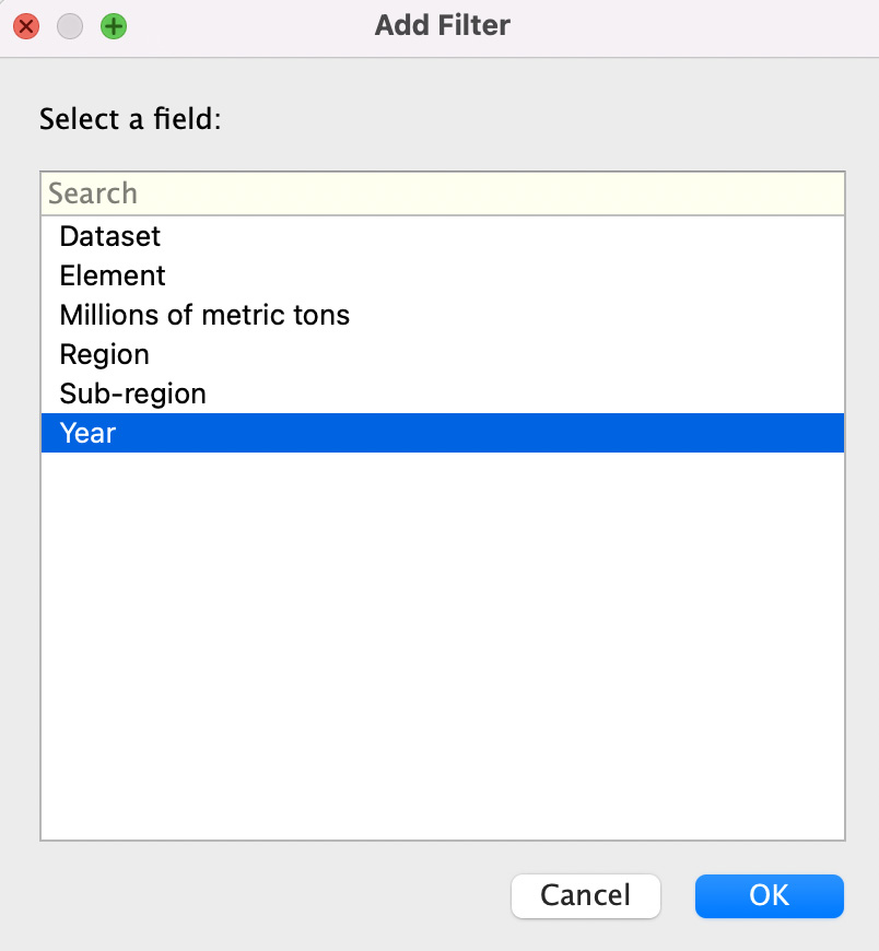
Figure 7.9 – The data extract filter dialog

12. Now we can limit the number of years we want in our data via the dialog box shown in Figure 7.10. For example, we could set the maximum range to 2026. For now, hit Cancel to dismiss the dialog box:

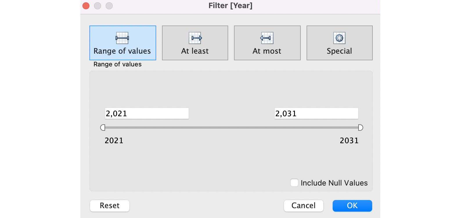
Figure 7.10 – The date filter dialog

13. The final pane of the data source page is simply called the left pane. It is on the left-hand side of the user interface, as shown in Figure 7.11:

Figure 7.11 – The left pane of the data source page

It contains three sections, as follows:

• Connections – A single workbook can have multiple data models. To add another data model to the same workbook, we can click on the Add button to add the new data.
• Sheets – Each sheet in a Microsoft Excel workbook shows up in this section. When we connect to databases, this section will show the tables in the database. Tableau treats each sheet of a Microsoft Excel workbook as a unique table. Use Data Interpreter only appears for Microsoft Excel and delimited files. We will look at this feature later in this chapter.
• New Union – We can use this feature to add additional rows of data from another table(s) to our model through a union. We will look at unions in greater detail in Chapter 8.

14. For our final step, we are going to save our workbook to use later in this chapter. From the File menu, choose Save and then name the workbook Chapter 7 Grain Data in the default location.

In this section, we explored how to use Microsoft Excel as a data source for our Tableau data model. Often, Microsoft Excel is a source of data for both personal analysis and in organizations due to the ubiquitous nature of Microsoft Excel and the ease of use for storing and updating data.

In the next section, we will look at how to connect to delimited files. Tableau treats these files similarly to Microsoft Excel.

Getting data from text (or delimited) files

Often, we get data for analysis in the form of delimited text files. Typically, the files are in the form of having the field names appear first, each separated by a character (or tab) to space or delimit them, followed by a carriage return. Then, the data itself comes next with that same character delimited by each value and a carriage return signifying the start of a new record. A common delimiter is a comma. Delimited files with a comma separator are called comma-separated value (CSV) files. If you open one of these files in Microsoft Excel or another spreadsheet application, they usually look like the file we saw in the previous section, that is, nicely arranged in a spreadsheet table format.

Often, we get delimited files, especially CSVs, as data exports from systems to which we do not have access. They might be available as public data such as our example from https://data.gov/ or be data dumped from internal or partner databases where the database administrator doesn’t allow us access. We will now bring in data from a CSV file to demonstrate this capability:

1. Open Tableau Desktop. From the Connect pane, under the To a File section, select Text file. Locate and highlight the Contribution_Amounts_for_Fiscal_Years_2002-03_to_2015-16.csv file and click on Open.
2. The metadata and data grids now look indistinguishable from how they would look if our data was in Microsoft Excel or any other data source that was structured this way. It should look like the screenshot in Figure 7.12:

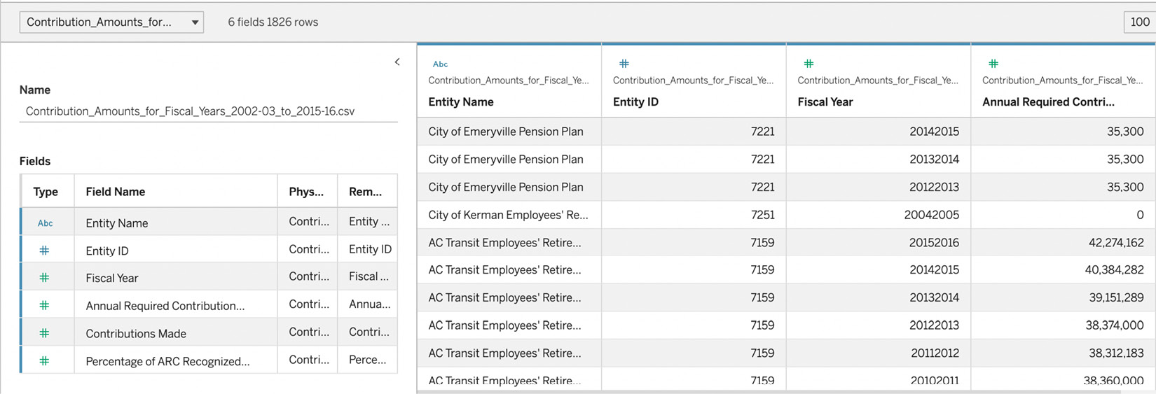
Figure 7.12 – Metadata and data grids for our CSV file

3. The only significant difference you will see will be in the left-hand pane. The section that said Sheets when we connected to Microsoft Excel will now say Files, as shown in Figure 7.13. The list contains all the files that are in the same directory as the file we just added to our model. This makes it easier to combine files through unions and joins if you keep them in the same file location:

Figure 7.13 – The left-hand pane example with a CSV file

4. We will conclude our exploration of connecting to delimited files here. Everything else about delimited files behaves like Microsoft Excel files.

In this section, we looked at delimited files (text files) in Tableau. We saw how they were the same as and different from Microsoft Excel files in terms of how Tableau handles them.

In the next section, we will look at spatial files. These allow for visual analysis with maps.

Importing geospatial file types to allow for visual analysis with maps

Tableau allows for geospatial analysis, that is, performing visual analytics on top of maps. Tableau can plot any data on a map when it has the latitude and longitude (latitude/longitude) values for the point. In Chapter 1, we also looked at the built-in geospatial field types in Tableau. Sometimes, we want our analysis to go beyond latitude/longitude and the built-in Tableau functions to look at custom, specific geospatial analysis. At the time of writing, Tableau allows for the import of Esri, GeoJSON, KML, KMZ, MapInfo, and TopoJSON files. We will now follow the steps required to connect to a GeoJSON file:

1. Open Tableau Desktop. From the Connect pane, under the To a File section, select Spatial file. Locate and select the DETROIT_BIKE_LANES.geojson file to highlight it and click on Open.
2. Scroll to the bottom of the metadata grid and you should see a field named Geometry, as shown in Figure 7.14:

Figure 7.14 – Metadata grid for the Detroit bikes spatial file

3. Let’s see what the Geometry field does by by first clicking on Sheet 1. Then, double-click on Geometry in the data pane. Drag the Name field to the Color card of the Marks card and drop it, as shown in Figure 7.15:

Figure 7.15 – Dragging the name and dropping it on the color card

4. The resulting visualization should look like the screenshot in Figure 7.16:

Figure 7.16 – The resulting map

This is a simple example of a spatial file showing the bike lanes in Detroit, each colored uniquely based on its name. We could combine this data with other information about Detroit to create a compelling analysis. For example, combining population data by neighborhood could help us to understand whether the bike lanes are in highly populated areas.

In this section, we explored how to bring in spatial files to create map-based analysis in Tableau. In the next section, we will discuss how to import statistical files into Tableau.

Creating data models from statistical files

Often, data is run through statistical models to have additional context added in the form of new columns. For example, you might have a file of customer comments collected via internal systems and through social media and review sites. Your organization might want to score custom sentiment over time by customer from this large amount of text. Tableau does not do this type of text analysis, but it could be done in commercial statistical software programs such as SPSS (Statistical Package for the Social Sciences) or SAS (Statistical Analysis System) or from open source programs such as R. These three programs have proprietary data export formats, although programmers will often export in CSV or other delimited exports.

Tableau can connect to SAS (*.sas7bdat), SPSS (*.sav), and R (*.rdata, *.rda) data files natively. To connect to these files, navigate to the Connect pane, under the To a File section, and select Statistical file. From this point, the experience is very similar to the experience of text (delimited) files.

In the next section, we will look at how to import JSON files. Typically, these files are generated from web applications and are worth future exploration due to their unique file format.

Creating data models from JSON files

JavaScript Object Notation (JSON) files are text-based files that are typically used to transfer data in web applications, usually from a database to a web page to convert into HTML for viewing. Because JSON files are sources of data, they can be opened by other applications, such as Tableau. We will now connect to a JSON file containing information from the United Nations Educational, Scientific, and Cultural Organization (UNESCO):

1. Open Tableau Desktop. From the Connect pane, under the To a File section, select JSON file. Locate and select the unece.json file to highlight it and click on Open.
2. You will be presented with a dialog box to select schema levels from the JSON file, as shown in Figure 7.17:

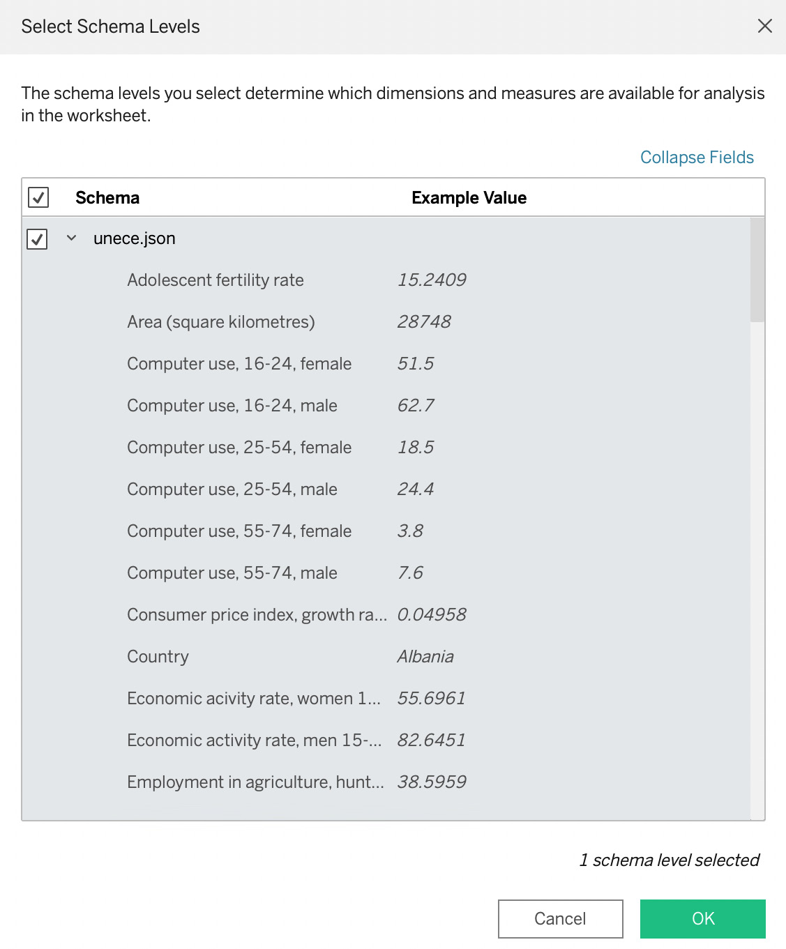
Figure 7.17 – The JSON schema selection dialog

Tableau works to flatten the schema to give us the spreadsheet table format that works best with Tableau. If the JSON file is organized into multiple schemas, you can select and deselect them at this point. In our example, the JSON file is organized into a single schema, which is selected by default. Click on OK to bring the JSON data into our data model.

3. At this point, the data from the JSON file will behave like data from a delimited text file and Microsoft Excel.

In this section, we looked at connecting to JSON files. JSON files are a file format that is used to transfer data, typically in web applications. JSON files have a schema in them that Tableau helps flatten to get the file in the format of a spreadsheet table, making data modeling and analysis easy in Tableau.

In the next section, we will look at the last of the file options for Tableau: the Portable Document Format (PDF) from Adobe.

Getting data from tables in PDF files

There are many use cases where it is helpful, or even necessary, to get data from tables contained in PDF documents. Financial data, including corporate filings and investment statements, can often only be found in PDFs. Another example is public policy data and other reports generated by governments. We will look at one of these examples next.

Before we begin this exercise, locate the hcilicensed-daycare-center760narrative11-13-15.pdf file from the location you saved it in on your computer. Open the document in your PDF reader of choice and take notice of the table found on page 7, as shown in Figure 7.18:

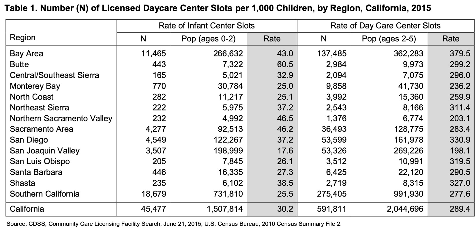
Figure 7.18 – Table 1 from page 7 of PDF

In the following steps, we will learn how to connect to the preceding table in Tableau Desktop:

1. Open Tableau Desktop. From the Connect pane, select PDF file, locate hcilicensed-daycare-center760narrative11-13-15.pdf, and press Open.
2. Tableau will now present a dialog box (Figure 7.19) where you can instruct Tableau to search the PDF document. In a long document, such as a corporate financial statement that might be over 100 pages in length, your PDF search will go much faster if you instruct Tableau which page(s) the table or tables you want to model are in the document. In our case, the PDF is only 7 pages long, so leave the default option of All and press OK:

Figure 7.19 – The Scan PDF File dialog

3. Tableau will now switch focus to the data source page and display all the tables that it found as per Figure 7.20:

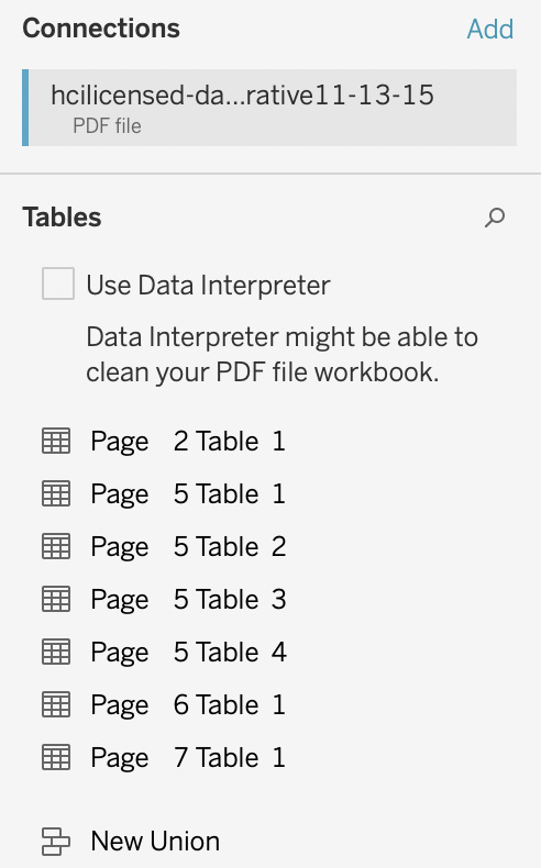
Figure 7.20 – Tables found in the PDF

4. Tableau found a total of 7 data tables in the PDF. The first six tables are Tableau interpreting the data behind the charts in the first six pages of the PDF. We are looking to pull in the data from the table on Page 7. To bring this data into our data model, double-click on Page 7 Table 1 to create the model.
5. Click on Sheet 1, and you will see all the fields from the table listed in the data pane. To recreate the basis of the table from Page 7 of the PDF, click on the following fields in this order: Region, N, Pop (ages 0-2), Rate, N1, Pop (ages 2-5), and Rate1. You should now have a sheet that looks like Figure 7.21:

Figure 7.21 – The rebuilt PDF table in Tableau

In Chapter 10, we will explore how to extend our data model. This will contain the formatting techniques that will allow us to make the preceding data table look close to the presentation in the PDF.

Now that we know how to connect to data in PDF documents, we can use PDF documents from financial, government, and other sources to incorporate into our data models without first needing to move that data to a spreadsheet or database.

In this section, we looked at how to connect to files. We looked at Microsoft Excel, delimited files, spatial files, statistical files, JSON files, and PDF tables, including examples of use cases for each type. There are many cases in both personal and organizational analysis where we might use these file types. In the next section, we will look at a data interpreter that can help us to save data modeling time and effort in certain types of Microsoft Excel and delimited files.

Dealing with preformatted reporting files with data interpreter and pivoting columns to rows

Often, data in Microsoft Excel and text fields comes with a few rows that act as headers to describe the data in the file. Looking at the SIPRI-Milex-data-1949-2021.xlsx file we downloaded from the GitHub repository, we can see that the data table doesn’t start until row 6. The first four rows describe the dataset with a blank fifth row, as shown in Figure 7.22:

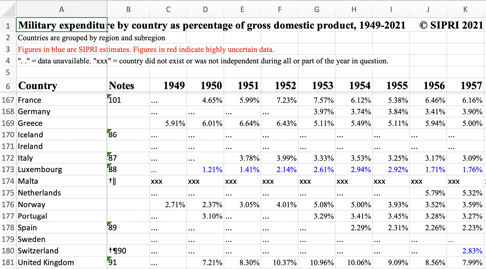
Figure 7.22 – Excel with header rows

Tableau is expecting the first row to be field names, one per column, and each of the other rows a record of data. Let’s open Tableau Desktop and connect to the file to see how we can bring it into a well-structured data model:

1. Open Tableau Desktop. From the Connect pane, select Microsoft Excel, locate SIPRI-Milex-data-1949-2021.xlsx, and click on Open.
2. Tableau will now switch the focus to the data source page. Double-click on the Share of GDP table to bring that data into Tableau. In the data details section of the Tableau user interface, you will see that Tableau is not automatically able to create a useable data model (Figure 7.23):

Figure 7.23 – Before the data interpreter

3. To fix this issue, we could manually delete the first five rows in the Excel file. If we were doing this analysis only once, that might be fine but what if we want to automate the process? This is where the data interpreter feature comes in. Click the checkbox next to Use Data Interpreter under the Sheets section of the Connections pane. After clicking on the checkbox, the user interface will change to Cleaned with Data Interpreter, as shown in Figure 7.24:

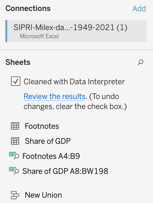
Figure 7.24 – Cleaned with Data Interpreter

4. In addition, the data details now show a data model that is much closer to the one we want (Figure 7.25):

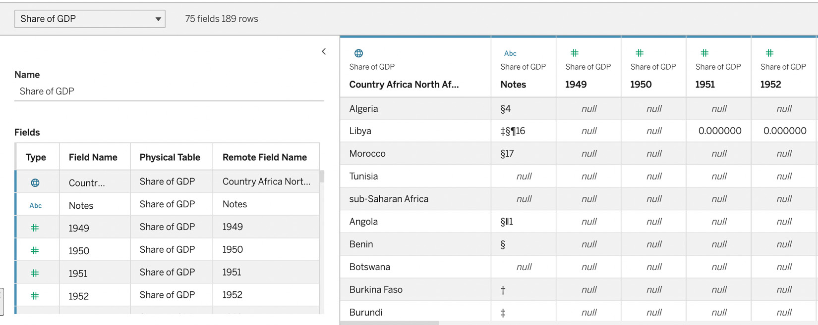
Figure 7.25 – Data details after Data Interpreter has been applied

5. This almost gives us the right data model with one step remaining. As you can see, the years go across the first row of the model and we want these years in a Date field with the values in a % of GDP field, making three fields, along with Country. The Notes field is not one we need, so we can eliminate it from our data model.
6. For our first step, we will rename the first field to just Country. Next to the first field, click on the ▼ symbol in the field header and click on Rename as per Figure 7.26. Type Country into the textbox that appears and hit Enter/Return:

Figure 7.26 – Renaming the field to Country

7. Next, we want to hide the Notes field as we don’t want it in our data model. Click on the ▼ symbol in the field header and select the Hide option, as shown in Figure 7.27:

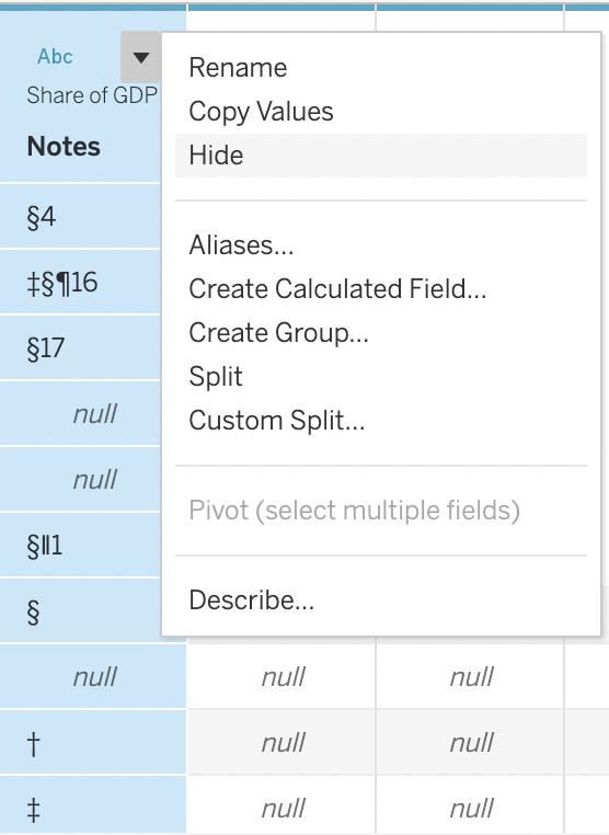
Figure 7.27 – Hiding the field

8. Our next step is to pivot the years into a Date field. In Chapter 4, we explored the pivot columns to rows feature of Tableau Prep Builder. We can also pivot columns to rows in Tableau Desktop, although the user experience is different. To pivot columns to rows, click on the column header of the 1949 field. Holding down the shift key, scroll all the way to the left, and click on the 2021 field to select all the date fields. Next, click on the ▼ next to the 2021 field header and select Pivot, as shown in Figure 7.28:

Figure 7.28 – Pivoting the dates

Note that both Tableau Desktop and Tableau Prep Builder can pivot columns to rows but only Tableau Prep Builder can pivot rows to columns. We will look at this and other differences between Tableau Desktop and Tableau Prep Builder in Chapter 15.

9. Our final step is to rename the Pivot Field Names field to Date and Pivot Field Values to % of GDP using the renaming technique in step 5 of this section. When you are finished, your data details pane should look like Figure 7.29:

Figure 7.29 – Final renaming

In this section, we learned how to create data models from Microsoft Excel and delimited files that come in the structure of pre-formatted reports by using the data interpreter feature and pivot columns to rows feature of Tableau Desktop. This allows us to save time and resources to automatically create data models from these types of data sources without needing manual intervention for every new file.

In the next section, we will look at how to connect to enterprise database servers, both on-premises and in the cloud.

Connecting to servers through installed connectors

Within an organizational setting, versus personal analysis, the data sources for Tableau data models are often contained in file stores, applications, and database servers. At the time of writing, using Tableau Desktop version 2022.2 on macOS. Tableau comes with 59 installed connectors for data servers. Installed connectors are connectors written and developed by Tableau and distributed with Tableau Desktop and Tableau Server and Cloud. Tableau Prep Builder also comes with installed connectors.

These connectors fall into the following general categories:

• On-premises database servers (for example, Oracle and Microsoft SQL Server)
• Cloud database servers (for example, Snowflake and Google BigQuery)
• Cloud applications (for example, Salesforce and ServiceNow)
• File shares (for example, Box and Google Drive)

Tableau maintains a list of current native connectors at https://help.tableau.com/current/pro/desktop/en-us/exampleconnections_overview.htm.

Connecting to these servers is beyond the scope of this book as it requires running servers that we would either need to set up, as in the case of cloud servers, or downloading and configuring, as in the case of on-premises servers.

Sometimes, connecting to these servers will require downloading database-specific drivers from the software vendor who creates the database. Tableau will direct you to the locations and instructions to download the necessary driver when you need it.

Once you have connected to the server, modeling in Tableau follows the same experience we used when exploring flat files.

Before leaving this section of the chapter, we will look at the two server connection experiences in Tableau. The first of these is via a dialog box within Tableau Desktop. An example of this style is Microsoft SQL Server:

1. Open Tableau Desktop. Click on Connect to Data. Select To a Server, More… and then Microsoft SQL Server, as shown in Figure 7.30:

Figure 7.30 – Connecting to Microsoft SQL Server

2. If you have the driver already installed, which is typically the default on computers running the Microsoft Windows operating system, you should see a dialog box that looks like the screenshot in Figure 7.31:

Figure 7.31 – The Microsoft SQL Server connection dialog

Once you enter the connection information in the dialog box, you will be taken to the data source page where you will be able to choose the tables just like choosing sheets from Microsoft Excel workbooks.

The other type of connection begins with authentication in a web browser. This is typical for data servers that use OAuth to manage user access. An example of a server that uses this style is Google Drive. If you connect to Google Drive, Tableau will open a browser window where you can connect using your Google account. At that point, Tableau will bring you back to the data source page where you can then start working with your data.

In this section, we explored the different types of installed data servers and how to connect to them. In the next section, we will look at how to connect to data via web data connectors, data server connectors created by Tableau partners, and generic connectors for data servers without native or partner connectors.

Connecting to servers through other connectors

In the previous section, we looked at how to connect to data servers through connectors developed by Tableau. As there are hundreds to thousands of potential data servers, it isn’t realistic for Tableau to develop connectors for all of them. In these cases, there are three other types of connectors:

• Additional connectors
• Web data connectors for connection to websites and web applications
• Generic ODBC and JDBC connectors

Let’s look at each of these types in detail.

Additional connectors

Additional connectors are listed in Tableau Desktop as Additional Connectors under To a Server. Typically, these connectors are developed by the Tableau software partner who also develops the data server they connect to, but they can be developed by Tableau and other third parties. At the time of writing, there are 21 additional connectors.

These connectors aren’t installed by default. Let’s look at how to install one of these connectors:

1. Open Tableau Desktop. From the Connect pane, select To a Server, and then select Qubole Hive by Qubole.
2. You should then see a dialog box like the screenshot in Figure 7.32. Note that there might be a newer version of the connector when you take this step, as additional connectors are updated regularly:

Figure 7.32 – The installation box for the Qubole connector

3. Click on Install and Restart Tableau. You should be taken to the https://extensiongallery.tableau.com/connectors page where you can download and install the Qubole connector. If your Tableau Desktop started without taking you to the connectors page, go to the URL in your browser, find the Qubole Hive card, and click on it. From this page, you will get instructions on how to download both the connector and the necessary drivers. We are not going to go through these steps as we do not have a Qubole database that we can connect to.
4. In Tableau Desktop, you should now see Qubole for Qubole Hive in the list of To a Server connectors, and your Additional Connectors should now have one less number. That is, after letting Tableau know you installed an additional connector, it behaves exactly like a regular server connector.

We have now looked at additional connectors. They behave the same as installed connectors except that they don’t come pre-installed with Tableau Desktop.

Next up, we will look at web data connectors. These are often shortened to their acronym, WDC, in Tableau documentation.

Web data connectors

Web data connectors (WDCs) are like additional connectors except that they pull data from the user interface layer of web applications, whereas server and additional connectors pull from the data layer of applications. In other words, you use WDCs to connect to data that is accessible over HTTP. A web data connector is an HTML file with JavaScript code. In all cases, Tableau will create an extract of the data it retrieves from the WDC.

Tableau makes it straightforward to create WDCs for web developers. Creating a WDC is beyond the scope of this book, so we will connect to an existing WDC.

We are going to use a WDC that accesses information from Tableau Public. Tableau Public is a free-to-use site to publish Tableau visualizations to share. This WDC was written by Andre de Vries:

1. Open Tableau Desktop. Click on Connect to Data. Select To a Server, More…, and then select Web Data Connector.
2. This will bring up a dialog, as shown in Figure 7.33. In the dialog, type in https://tableau-public-api.wdc.dev/ and press Enter:

Figure 7.33 – Web data connector dialog

3. After pressing Enter, the dialog box should change to look like the screenshot in Figure 7.34. If you have a Tableau Public profile, you can enter your username where it says to Enter Username. If not, you can enter kirk.munroe or your favorite Tableau Public author. After entering a username, press Get Data:

Figure 7.34 – Enter a username to retrieve stats from Tableau Public

4. When the data comes back, you will be on the data source page. In the upper-right corner of the screen, you should notice that the only option is Extract. Tableau does not give the option to continually query the web application live as this type of query would be very slow.

In this section, we explored web data connectors to see how they allow us to get data from websites and web applications. We looked at one example of a WDC, one that allows us to retrieve data from http://public.tableau.com. In practice, we might need to get data from a web application that does not have a server connection. In these cases, we can write our own or get a web developer to write one for us. Creating a WDC is beyond the scope of this book. Instructions on how to build a WDC can be found via the link in the bottom-right corner of the WDC dialog box, as shown in Figure 7.33 and step 3 of this section.

Next, we will look at how to connect to databases that do not have native or additional connectors.

Connecting to databases without a listed connection

As we discussed earlier in this chapter, Tableau provides many server connectors – both natively and through additional connectors. At the time of writing, Tableau has a total of 80 connectors for Tableau Desktop 2022.2. However, there are hundreds more databases available. If you are in a position where you need to retrieve data from one of these databases to build your data model, the generic Other Databases (JDBC) or Other Databases (ODBC) drivers might be your answer.

ODBC is an acronym for Open Database Connectivity. It is a standard that allows client software, such as Tableau, to query database management systems (DBMS). It is written for client software written in Microsoft technology (for example, C++ and C#). JDBC is an acronym for Java Database Connectivity. It serves the same purpose as ODBC except being written for clients written in Java.

In the case of Tableau Desktop (and Tableau Server and Cloud), the client can use both ODBC and JDBC, so the choice mostly comes down to the DBMS that is being accessed. How do we know which one to use? We should research the DBMS that we are connecting to and see whether they prefer one over the other. If this isn’t a factor, it is worth trying both connectors to see which one offers better performance. We should always consider the type of connection we will keep when considering the connector, too. It could be that one of the connectors is faster for smaller query result sets and the other faster for fetching a larger bulk of records. In this example, the first choice is better for live connections, and the second is better if we know that we will be using a data extract.

In all cases where an installed or additional connector exists in Tableau, always choose the named connector. The purpose-built named connectors will yield faster query results and might offer additional features that aren’t available in the generic ODBC and JDBC standards.

Connecting to the Tableau data server

Typically, Tableau Server and Cloud are thought of as servers that provide web interfaces to create, share, and manage data analytics, typically in the form of dashboards. Tableau Server and Cloud also provide other capabilities including acting as a data server.

Tableau has two data server features. The first of these features is only available with the Data Management licensing and is called virtual connections. Virtual connections aren’t data models but a method of accessing a database through Tableau Server and Cloud. We explored virtual connections in Chapter 2.

The more common feature is the published data source feature. Published data sources are the best practice for sharing data models with others in your organization. We will be looking at extending the metadata of published data sources in Chapter 10. We also created our first published data source from Tableau Prep Builder in the previous chapter, Chapter 6. Let’s look at how we can create a published data source from Tableau Desktop, and then we will see how we can connect to our published data sources when we open Tableau Desktop:

1. Open Tableau Desktop. Open the Chapter 7 Grain Data workbook that we saved earlier in this chapter. This workbook can be opened from the home screen of Tableau Desktop or by navigating to the File menu and then clicking on Open.
2. Once the workbook is open, go to the Server menu, then Publish Data Source, then Sheet1 (GrainDemandProduction), as shown in Figure 7.35. If you aren’t signed into your Tableau Server or Cloud, you will need to do that first from the first menu option. Also, Sheet1 (GrainDemandProduction) is the default name of the data source. Additionally, you can change it from the data source page screen:

Figure 7.35 – The Publish Data Source menu

3. You will be presented with a dialog box, as shown in Figure 7.36. First, you need to pick a project from your Server or Tableau Cloud site. In this case, we will leave the project as Default as long as you have permission to publish to that project. If not, use the drop-down menu to choose a project that you do have permission to publish. In addition to the data source page, we have the option to rename the published data source here. For now, we will leave all the defaults and explore them in greater detail in Chapter 10:

Figure 7.36 – The Publish Data Source dialog

4. The data source page will show up in a browser window after being published as shown in Figure 7.37. If you are using Tableau cloud, you will see a warning about needing to use Tableau Bridge. We will explore Tableau Bridge in further detail in Chapter 14. For now, you can dismiss the browser window. Close Tableau Desktop without saving:

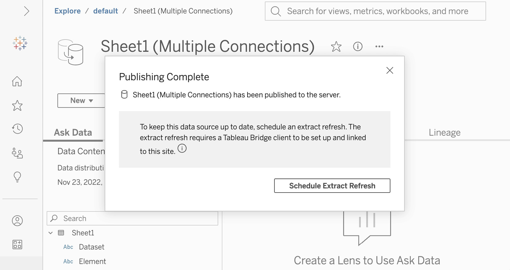
Figure 7.37 – Tableau data source page

5. Open Tableau Desktop. From the Connect pane, select Tableau Server from the Search for Data section, as shown in Figure 7.38. You can make this selection whether you are using Tableau Server or Tableau Cloud:

Figure 7.38 – Connecting to the Tableau published data source

6. When the dialog comes up to connect, you should see the AMER Sales Transactions we created in Chapter 6 as well as the Sheet1 (GrainDemandProduction) data source we created in step 4 of this section, as shown in Figure 7.39. Select Sheet1 (GrainDemandProduction) and press Connect. You have now connected to your first published data source in Tableau Desktop:

Figure 7.39 – Connecting to a published data source

In this section, we created our first published data source from Tableau Desktop and connected to our first published data source in Tableau Desktop. We will be exploring published data sources in more detail in the upcoming chapters. Published data sources are one of the key components of Tableau data modeling.

Summary

In this chapter, we learned about the different data sources available to Tableau Desktop.

In the first section, we looked at the different file types that can be data sources for Tableau. We imported data to create data models from Microsoft Excel, CSV files, JSON files, spatial files, and tables from PDF files.

We looked at the different types of servers that Tableau connects to, including native connectors, additional connectors, and generic ODBC and JDBC connectors when our data server is not listed. Additionally, we looked at web data connectors for creating models from the data on web pages and web applications.

In the final section, we looked at creating and connecting to Tableau published data sources, one of the key components for data modeling at scale in Tableau.

This chapter focused on the building blocks of data modeling in Tableau – connecting to data. In the next three chapters, we will look at how to extend and scale our data models by combining multiple data sources into a single model and then securing and sharing that model. The next chapter will focus on extending data models through logical tables.