
Chapter 21
Sensors
Sensors provide us with a means of generating signals that can be used as inputs to electronic circuits. The things that we might want to sense include physical parameters such as temperature, light level, and pressure. Being able to generate an electrical signal that accurately represents these quantities allows us not only to measure and record these values but also to control them.
Sensors are, in fact, a subset of a larger family of devices known as transducers so we will consider these before we look at sensors and how we condition the signals that they produce in greater detail. We begin, however, with a brief introduction to the instrumentation and control systems in which sensors, transducers, and signal conditioning circuits are used
21.1 Instrumentation and Control Systems
Figure 21.1 shows the arrangement of an instrumentation system. The physical quantity to be measured (e.g., temperature) acts upon a sensor that produces an electrical output signal. This signal is an electrical analog of the physical input but note that there may not be a linear relationship between the physical quantity and its electrical equivalent. Because of this and since the output produced by the sensor may be small or may suffer from the presence of noise (i.e., unwanted signals) further signal conditioning will be required before the signal will be at an acceptable level and in an acceptable form

Figure 21.1 Instrumentation and control system
for signal processing, display and recording. Furthermore, because the signal processing may use digital rather than analog signals an additional stage of analog-to-analog conversion may be required.
Figure 21.1(B) shows the arrangement of a control system. This uses negative feedback in order to regulate and stabilize the output. It thus becomes possible to set the input or demand (i.e., what we desire the output to be) and leave the system to regulate itself by comparing it with a signal derived from the output (via a sensor and appropriate signal conditioning).
A comparator is used to sense the difference in these two signals and where any discrepancy is detected the input to the power amplifier is adjusted accordingly. This signal is referred to as an error signal (it should be zero when the output exactly matches the demand). The input (demand) is often derived from a simple potentiometer connected across a stable DC voltage source while the controlled device can take many forms (e.g., a DC motor, linear actuator, heater, etc.).
21.2 Transducers
Transducers are devices that convert energy in the form of sound, light, heat, etc., into an equivalent electrical signal, or vice versa.
Before we go further, let’s consider a couple of examples that you will already be familiar with. A loudspeaker is a transducer that converts low-frequency electric current into audible sounds. A microphone, on the other hand, is a transducer that performs the reverse function, i.e., that of converting sound pressure variations into voltage or current. Loudspeakers and microphones can thus be considered as complementary transducers.
Transducers may be used as both inputs to electronic circuits and outputs from them. From the two previous examples, it should be obvious that a loudspeaker is an output transducer designed for use in conjunction with an audio system, whereas a microphone is an input transducer designed for use with a recording or sound reinforcing system.
There are many different types of transducer and Tables 21.1 and 21.2 provide some examples of transducers that can be used to input and output three important physical quantities; sound, temperature, and angular position.

Figure 21.2 A selection of thermocouple probes
Table 21.1 Some examples of input transducers
| Physical quantity | Input transducer | Notes |
| Sound (pressure change) | Dynamic microphone (see Figure 21.3) | Diaphragm attached to a coil is suspended in a magnetic field. Movement of the diaphragm causes current to be induced in the coil. |
| Temperature | Thermocouple (see Figure 21.2) | Small e.m.f. generated at the junction between two dissimilar metals (e.g., copper and constantan). Requires reference junction and compensated cables for accurate measurement |
| Angular position | Rotary potentiometer | Fine wire resistive element is wound around a circular former. Slider attached to the control shaft makes contact with the resistive element. A stable DC voltage source is connected across the ends of the potentiometer. Voltage appearing at the slider will then be proportional to angular position. |
Table 21.2 Some examples of output transducers
| Physical quantity | Output transducer | Notes |
| Sound (pressure change) | Loudspeaker (see Figure 21.3) | Diaphragm attached to a coil is suspended in a magnetic field. Current in the coil causes movement of the diaphragm which alternately compresses and rarefies the air mass in front of it. |
| Temperature | Heating element (resistor) | Metallic conductor is wound onto a ceramic or mica former. Current flowing in the conductor produces heat. |
| Angular position | Rotary potentiometer | Multi-phase motor provides precise rotation in discrete steps of 15° (24 steps per revolution), 7.5° (48 steps per revolution) and 1.8° (200 steps per revolution) |
21.3 Sensors
A sensor is a special kind of transducer that is used to generate an input signal to a measurement, instrumentation or control system. The signal produced by a sensor is an electrical analogy of a physical quantity, such as distance, velocity, acceleration, temperature, pressure, light level, etc. The signals returned from a sensor, together with control inputs from the user or controller (as appropriate) will subsequently be used to determine the output from the system. The choice of sensor is governed by a number of factors including accuracy, resolution, cost, and physical size.

Figure 21.3 A selection of audible transducers
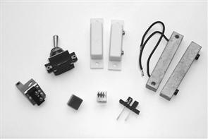
Figure 21.4 Various switch sensors
Sensors can be categorized as either active or passive. An active sensor generates a current or voltage output. A passive transducer requires a source of current or voltage and it modifies this in some way (e.g., by virtue of a change in the sensor’s resistance). The result may still be a voltage or current but it is not generated by the sensor on its own.
Sensors can also be classed as either digital or analog. The output of a digital sensor can exist in only two discrete states, either “on” or “off”, “low” or “high”, “logic 1” or “logic 0”, etc. The output of an analog sensor can take any one of an infinite number of voltage or current levels. It is thus said to be continuously variable. Table 21.3 provides details of some common types of sensor.

Figure 21.5 Resistive linear position sensor

Figure 21.6 Various temperature and gas sensors
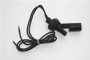
Figure 21.7 Liquid level float switch

Figure 21.8 Various optical and light sensors

Figure 21.9 Liquid flow sensor (digital output)
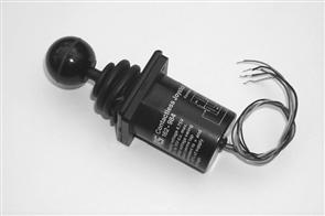
Figure 21.10 Contactless joystick
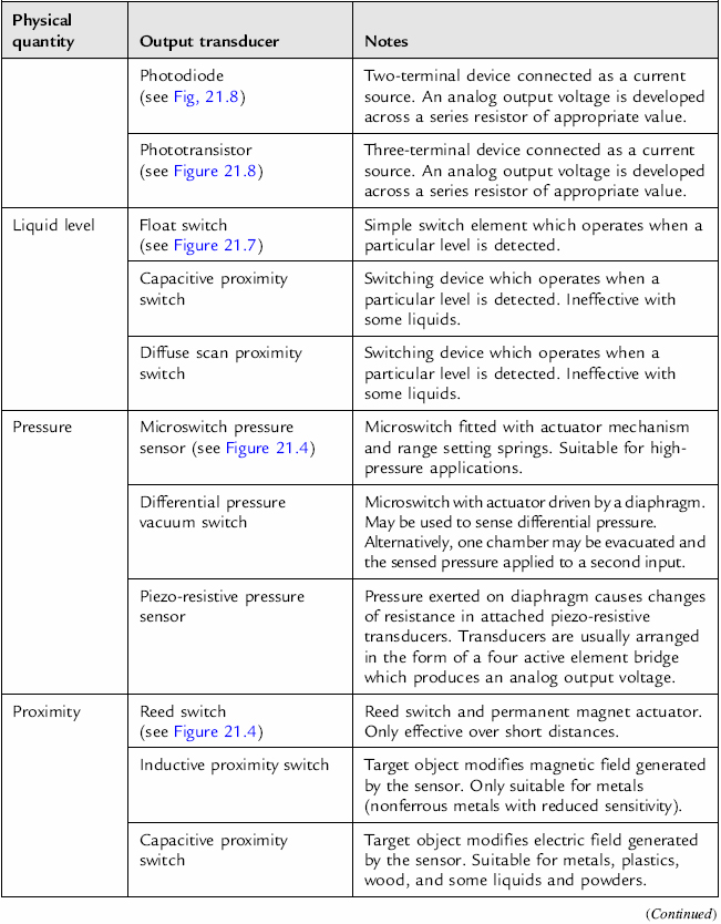
Table 21.3 Some examples of output transducers

21.4 Switches
Switches can be readily interfaced to electronic circuits in order to provide manual inputs to the system. Simple toggle and push-button switches are generally available with normally open (NO), normally closed (NC), or changeover contacts. In the latter case, the switch may be configured as either an NO or an NC type, depending upon the connections used.
Toggle, lever, rocker, rotary, slide, and push-button types are all commonly available in a variety of styles. Illuminated switches and key switches are also available for special applications. The choice of switch type will obviously depend upon the application and operational environment.
An NO switch or push-button may be interfaced to a logic circuit using nothing more than a single pull-up resistor as shown in Figure 21.11.

Figure 21.11 Interfacing a normally open switch or push-button to a digital input port
The relevant bit of the input will then return 0 when the switch contacts are closed (i.e., when the switch is operated or where the pushbutton is depressed). When the switch is inactive, the logic input will return 1.
Unfortunately, this simple method of interfacing has a limitation when the state of a switch is being sensed regularly (e.g., during program execution). However, a typical application which is unaffected by this problem is that of using one or more PCB mounted switches (e.g., a DIL switch package) to configure a logic system in one of a number of preset modes. In such cases, the switches would be set once only and the software would read the state of the switches and use the values returned to initially configure the system. Thereafter, the state of the switches would then only be changed in order to modify the operational parameters of the system (e.g., when changing input sensors or output transducers). A typical DIL switch input interface to a digital input port is shown in Figure 21.12.
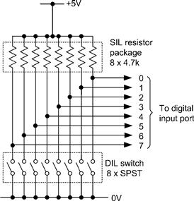
Figure 21.12 Interfacing a DIL switch input to a digital input port
As mentioned earlier, the simple circuit of Figure 21.11 is unsuitable for use when the state of the switch is regularly changing. The reason for this is that the switching action of most switches is far from “clean” (i.e., the switch contacts make and break several times whenever the switch is operated). This may not be a problem when the state of a switch remains static during program execution but it can give rise to serious problems when dealing with, for example, an operator switch bank or keypad.
The contact “bounce” that occurs when a switch is operated results in rapid making and breaking of the switch until it settles into its new state. Figure 21.13 shows the waveform generated by the simple switch input circuit of Figure 21.11 as the contacts close. The spurious states can cause problems if the switch is sensed during the period in which the switch contacts are in motion, and hence steps must be taken to minimize the effects of bounce. This may be achieved by using some extra circuitry in the form of a debounce circuit or by including appropriate software delays (of typically 4 to 20 ms) so that spurious switching states are ignored. We shall discuss these two techniques separately.
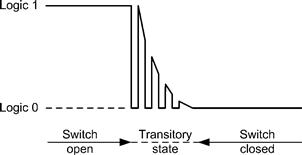
Figure 21.13 Typical waveform produced by a switch closure
Immunity to transient switching states is generally enhanced by the use of active-low inputs (i.e., a logic 0 state at the input is used to assert the condition required). The debounce circuit shown in Figure 21.14 is adequate for most toggle, slide and push-button type switches. The value of the 100Ω resistor takes into account the low-state sink current required by IC1 (normally 1.6 mA for standard TTL and 400 μA for LS-TTL). This resistor should not be allowed to exceed approximately 470Ω in order to maintain a valid logic 0 input state. The values quoted generate an approximate 1 ms delay (during which the switch contacts will have settled into their final state). It should be noted that, on power-up, this circuit generates a logic 1 level for approximately 1 ms before the output reverts to a logic 0 in the inactive state. The circuit obeys the following state table:
| Switch condition | Logic output |
| closed | 1 |
| open | 0 |

Figure 21.14 Simple debounce circuit
An alternative, but somewhat more complex, switch de-bouncing arrangement is shown in Figure 21.15. Here a single-pole double-throw (SPDT) changeover switch is employed. This arrangement has the advantage of providing complementary outputs and it obeys the following state table:
| Switch condition | Q |
| Q → 1 | 1 |
| Q → 0 | 0 |
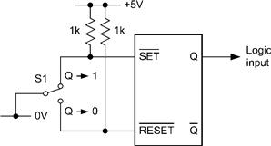
Figure 21.15 Debounce circuit based on an RS bistable
Rather than use an integrated circuit RS bistable in the configuration of Figure 21.15 it is often expedient to make use of “spare” two-input NAND or NOR gates arranged to form bistables using the circuits shown in Figs 21.16(A) and 21.16(B), respectively. Figure 21.17 shows a rather neat extension of this theme in the form of a touch-operated switch. This arrangement is based on a 4011 CMOS quad two-input NAND gate (though only two gates of the package are actually used in this particular configuration).
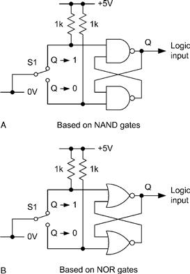
Figure 21.16 Alternative switch debounce circuits: (A) based on NAND gates; (B) based on NOR gates
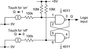
Figure 21.17 Touch-operated switch
Finally, it is some times necessary to generate a latching action from a normally-open push-button switch. Figure 21.18 shows an arrangement in which a 74LS73 JK bistable is clocked from the output of a debounced switch.
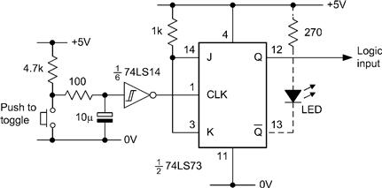
Figure 21.18 Latching action switch
Pressing the switch causes the bistable to change state. The bistable then remains in that state until the switch is depressed a second time. If desired, the complementary outputs provided by the bistable may be used to good effect by allowing the unused output to drive an LED. This will become illuminated whenever the Q output is high.
21.5 Semiconductor Temperature Sensors
Semiconductor temperature sensors are ideal for a wide range of temperature-sensing applications. The popular AD590 semiconductor temperature sensor, for example, produces an output current that is proportional to absolute temperature and which increases at the rate of 1 μA/K. The characteristic of the device is illustrated in Figure 21.19. The AD590 is laser trimmed to produce a current of 298.2 μA (±2.5 μA) at a temperature of 298.2°C (i.e., 25°C). A typical interface between the AD590 and an analog input is shown in Figure 21.20.

Figure 21.19 AD590 semiconductor temperature sensor characteristic

Figure 21.20 Typical input interface for the AD590 temperature sensor (the output voltage will increase at the rate of 10 mV per °C
21.6 Thermocouples
Thermocouples comprise a junction of dissimilar metals which generate an e.m.f. proportional to the temperature differential which exists between the measuring junction and a reference junction. Since the measuring junction is usually at a greater temperature than that of the reference junction, it is sometimes referred to as the hot junction. Furthermore, the reference junction (i.e., the cold junction) is often omitted in which case the sensing junction is simply terminated at the signal conditioning board. This board is usually maintained at, or near, normal room temperatures.
Thermocouples are suitable for use over a very wide range of temperatures (from −100°C to +1100°C). Industry standard “type K” thermocouples comprise a positive arm (conventionally colored brown) manufactured from nickel/chromium alloy while the negative arm (conventionally colored blue) is manufactured from nickel/aluminum.
The characteristic of a type K thermocouple is defined in BS 4937 Part 4 of 1973 (International Thermocouple Reference Tables) and this standard gives tables of e.m.f. versus temperature over the range 0°C to +1100. In order to minimize errors, it is usually necessary to connect thermocouples to appropriate signal conditioning using compensated cables and matching connectors. Such cables and connectors are available from a variety of suppliers and are usually specified for use with type K thermocouples. A selection of typical thermocouple probes for high temperature measurement was shown earlier in Figure 21.2.
21.7 Threshold Detection
Analog sensors are sometimes used in situations where it is only necessary to respond to a pre-determined threshold value. In effect, a two-state digital output is required. In such cases a simple one-bit analog-to-digital converter based on a comparator can be used. Such an arrangement is, of course, very much simpler and more cost-effective than making use of a conventional analog input port!
Simple threshold detectors for light level and temperature are shown in Figure 21.21, 21.22, and 21.24. These circuits produce TTL-compatible outputs suitable for direct connection to a logic circuit or digital input port.

Figure 21.21 Light-level threshold detector based on a light-dependent resistor (LDR)
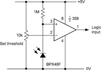
Figure 21.22 Light level threshold detector based on a photodiode

Figure 21.23 Comparison of the spectral response of an LDR and some common photodiodes
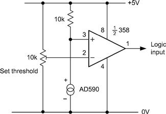
Figure 21.24 Temperature threshold detector based on an AD590 semiconductor temperature sensor
Figure 21.21 shows a light level threshold detector based on a comparator and light-dependent resistor (LDR). This arrangement generates a logic 0 input whenever the light level exceeds the threshold setting, and vice versa. Figure 21.22 shows how light level can be sensed using a photodiode. This circuit behaves in the same manner as the LDR equivalent but it is important to be aware that circuit achieves peak sensitivity in the near infrared region. Figure 21.23 shows how the spectral response of a typical light-dependent resistor (NORP12) compares with that of a conventional photodiode (BPX48). Note that the BPX48 can also be supplied with an integral daylight filter (BPX48F).
Figure 21.24 shows how temperature thresholds can be sensed using the AD590 sensor described earlier. This arrangement generates a logic 0 input whenever the temperature level exceeds the threshold setting, and vice versa.
21.8 Outputs
Having dealt at some length with input sensors, we shall now focus our attention on output devices (such as relays, loudspeakers, and LED indicators) and the methods used for interfacing them. Integrated circuit output drivers are available for more complex devices, such as LCD displays and stepper motor. However, many simple applications will only require a handful of components in order to provide an effective interface.
21.9 LED Indicators
Indicators based on light emitting diodes (LEDs) are inherently more reliable than small filament lamps and also consume considerably less power. They are ideal for providing visual status and warning displays. LEDs are available in a variety of styles and colors and “high brightness” types can be employed where high-intensity displays are required.
A typical red LED requires a current of around 10 mA to provide a reasonably bright display and such a device may be directly driven from a buffered digital output port. Different connections are used depending upon whether the LED is to be illuminated for a logic 0 or logic 1 state. Several possibilities are shown in Figure 21.25.
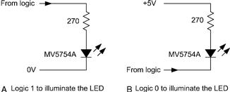
Figure 21.25 Driving an LED from a buffered logic gate or digital I/O port
Where drive current is insufficient to operate an LED, an auxiliary transistor can be used as shown in Figure 21.26. The LED will operate when the output from a logic circuit card is taken to logic 1 and the operating current should be approximately 15 mA (thereby providing a brighter display than the arrangements previously described). The value of LED series resistance will be dependent upon the supply voltage and can be selected from the data shown in Table 21.4.

Figure 21.26 Using an auxiliary transistor to drive an LED where current drive is limited
Table 21.4 Typical waveform produced by a switch closure
| Voltage | Series resistance (all 0.25W) |
| 3V to 4V | 100Ω |
| 4V to 5V | 150Ω |
| 5V to 8V | 220Ω |
| 8V to 12V | 470Ω |
| 12V to 15V | 820Ω |
| 15V to 20V | 1.2kΩ |
| 20V to 28V | 1.5kΩ |
21.10 Driving High-Current Loads
Due to the limited output current and voltage capability of most standard logic devices and I/O ports, external circuitry will normally be required to drive anything other than the most modest of loads. Figure 21.27 shows some typical arrangements for operating various types of medium- and high-current load. Figure 21.27(B) shows how an NPN transistor can be used to operate a low-power relay. Where the relay requires an appreciable operating current (say, 150 mA, or more) a plastic encapsulated Darlington power transistor should be used as shown in Figure 21.27(B). Alternatively, a power MOSFET may be preferred, as shown in Figure 21.27(C). Such devices offer very low values of “on” resistance coupled with a very high “off ” resistance. Furthermore, unlike conventional bipolar transistors, a power FET will impose a negligible load on an I/O port. Figure 21.27(D) shows a filament lamp driver based on a plastic Darlington power transistor. This circuit will drive lamps rated at up to 24V, 500 mA. Finally, where visual indication of the state of a relay is desirable it is a simple matter to add an LED indicator to the driver stage, as shown in Figure 21.28.

Figure 21.27 Typical medium- and high-current driver circuits: (A) transistor low-current relay driver; (B) Darlington medium/high-current relay driver; (C) MOSFET relay driver; (D) Darlington low-voltage filament lamp driver
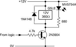
Figure 21.28 Showing how an LED indicator can easily be added to a relay driver
21.11 Audible Outputs
Where simple audible warnings are required, miniature piezoelectric transducers may be used. Such devices operate at low voltages (typically in the range 3V to 15V) and can be interfaced with the aid of a buffer, open-collector logic gate, or transistor. Figure 21.29(A)–(C) show typical interface circuits which produce an audible output when the port output line is at logic 1.
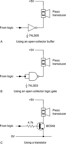
Figure 21.29 Audible output driver circuits
Where a pulsed rather than continuous audible alarm is required, a circuit of the type shown in Figure 21.30 can be employed. This circuit is based on a standard 555 timer operating in astable mode and operates at approximately 1 Hz. A logic 1 from the port output enables the 555 and activates the pulsed audio output.
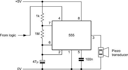
Figure 21.30 Audible alarm circuit based on a 555 astable oscillator and a piezoelectric transducer
Finally, the circuit shown in Figure 21.31 can be used where a conventional moving-coil loudspeaker is to be used in preference to a piezoelectric transducer. This circuit is again based on the 555 timer and provides a continuous output at approximately 1 kHz whenever the port output is at logic 1.

Figure 21.31 Audible alarm circuit based on a 555 astable oscillator and a 40Ω loudspeaker
21.12 Motors
Circuit arrangements used for driving DC motors generally follow the same lines as those described earlier for use with relays. As an example, the circuits shown in Figure 21.32 show how a Darlington driver and a power MOSFET can be used to drive a low-voltage DC motor. These circuits are suitable for use with DC motors rated at up to l2V with stalled currents of up to 3A. In both cases, a logic 1 from the output port will operate the motor.

Figure 21.32 Motor driver circuits
21.13 Driving Mains Connected Loads
Control systems are often used in conjunction with mains connected loads. Modern solid-state relays (SSRs) offer superior performance and reliability when compared with conventional relays in such applications. SSRs are available in a variety of encapsulations (including DIL, SIL, flat-pack, and plug-in octal) and may be rated for RMS currents between lA and 40A.
In order to provide a high degree of isolation between input and output, SSRs are optically coupled. Such devices require minimal input currents (typically 5 mA, or so, when driven from 5V) and they can thus be readily interfaced with an I/O port that offers sufficient drive current. In other cases, it may be necessary to drive the SSR from an unbuffered I/O port using an open-collector logic gate. Typical arrangements are shown in Figure 21.33. Finally, it is important to note that, when an inductive load is to be controlled, a snubber network should be fitted, as shown in Figure 21.34.

Figure 21.33 Interface circuits for driving solid-state relays

Figure 21.34 Using a snubber circuit with an inductive load