
Chapter 9. Understanding EIGRP Concepts
This chapter covers the following exam topics:
2.0 Routing Technologies
2.2 Compare and contrast distance vector and link-state routing protocols
2.3 Compare and contrast interior and exterior routing protocols
2.6 Configure, verify, and troubleshoot EIGRP for IPv4 (excluding authentication, filtering, manual summarization, redistribution, stub)
This chapter takes an in-depth look at a second option for an IPv4 routing protocol: the Enhanced Interior Gateway Routing Protocol, or EIGRP. This Cisco-proprietary routing protocol uses configuration commands much like Open Shortest Path First (OSPF), with the primary difference being that EIGRP configuration does not need to refer to an area. However, EIGRP does not use link-state (LS) logic, instead using some advanced distance vector (DV) logic. So, this chapter discusses quite a bit of detail about how routing protocols work and how EIGRP works before moving on to EIGRP configuration.
This chapter breaks the topics into two major sections. The first looks at some distance vector concepts, comparing some of the basic features of RIPv2 with the more advanced features of EIGRP. The second major section looks at the specifics of EIGRP operation, including EIGRP neighbors, exchanging routing information, and calculating the currently best routes to reach each possible subnet.
“Do I Know This Already?” Quiz
Take the quiz (either here, or use the PCPT software) if you want to use the score to help you decide how much time to spend on this chapter. The answers are at the bottom of the page following the quiz, and the explanations are in DVD Appendix C and in the PCPT software.
1. Which of the following distance vector features prevents routing loops by causing the routing protocol to advertise only a subset of known routes, as opposed to the full routing table, under normal stable conditions?
a. Route poisoning
b. Poison reverse
c. DUAL
d. Split horizon
2. Which of the following distance vector features prevents routing loops by advertising an infinite metric route when a route fails?
a. Dijkstra SPF
b. DUAL
c. Split horizon
d. Route poisoning
3. Routers A and B use EIGRP. How does router A watch for the status of router B so that router A can react if router B fails?
a. By using EIGRP Hello messages, with A needing to receive periodic Hello messages to believe B is still working.
b. By using EIGRP update messages, with A needing to receive periodic update messages to believe B is still working.
c. Using a periodic ping of B’s IP address based on the EIGRP neighbor timer.
d. None of the other answers are correct.
4. Which of the following affect the calculation of EIGRP metrics when all possible default values are used? (Choose two answers.)
a. Bandwidth
b. Delay
c. Load
d. Reliability
e. MTU
f. Hop count
5. Which of the following is true about the concept of EIGRP feasible distance?
a. A route’s feasible distance is the calculated metric of a feasible successor route.
b. A route’s feasible distance is the calculated metric of the successor route.
c. The feasible distance is the metric of a route from a neighboring router’s perspective.
d. The feasible distance is the EIGRP metric associated with each possible route to reach a subnet.
6. Which of the following is true about the concept of EIGRP reported distance?
a. A route’s reported distance is the calculated metric of a feasible successor route.
b. A route’s reported distance is the calculated metric of the successor route.
c. A route’s reported distance is the metric of a route from a neighboring router’s perspective.
d. The reported distance is the EIGRP metric associated with each possible route to reach a subnet.
Answers to the “Do I Know This Already?” quiz:
Foundation Topics
EIGRP and Distance Vector Routing Protocols
IPv4’s long history has resulted in many competing interior gateway protocols (IGP). Each of those different IPv4 IGPs differs in some ways, including the underlying routing protocol algorithms like link state and distance vector. This first section of the chapter looks at how EIGRP acts like distance vector routing protocols to some degree, while at the same time, EIGRP does not fit easily into any category at all.
In particular, this first section positions EIGRP against the other common IPv4 routing protocols. Then this section looks at basic DV concepts as implemented with RIP. Using the simpler RIP to learn the basics helps the discussion focus on the DV concepts. This section ends then with a discussion of how EIGRP uses DV features but in a more efficient way than RIP uses them.
Introduction to EIGRP
Historically speaking, the first IPv4 routing protocols used DV logic. RIP Version 1 (RIPv1) was the first popularly used IP routing protocol, with the Cisco-proprietary Interior Gateway Routing Protocol (IGRP) being introduced a little later, as shown in Figure 9-1.

By the early 1990s, business and technical factors pushed the IPv4 world toward a second wave of better routing protocols. RIPv1 and IGRP had some technical limitations, even though they were great options for the technology levels of the 1980s. The world needed better routing protocols due to the widespread adoption and growth of TCP/IP in enterprise networks in the 1990s. Many enterprises migrated away from older vendor-proprietary networks to instead use networks built with routers, LANs, and TCP/IP. These businesses needed better performance from their routing protocols, including better metrics and better convergence. All these factors led to the introduction of a new wave of IPv4 interior routing protocols: RIP Version 2 (RIPv2), OSPF, and EIGRP.
Even today, EIGRP and OSPF remain the two primary competitors as the IPv4 routing protocol to use in a modern enterprise IPv4 internetwork. RIPv2 has fallen away as a serious competitor, in part due to its less robust hop-count metric, and in part due to its slower (worse) convergence time. Even today, you can walk in to most corporate networks and find either EIGRP or OSPF as the routing protocol used throughout the network.
So, with so many IPv4 routing protocols, how does a network engineer choose which routing protocol to use? Well, consider two key points about EIGRP that drive engineers toward wanting to use it:

![]() EIGRP uses a robust metric based on both link bandwidth and link delay, so routers make good choices about the best route to use (see Figure 9-2).
EIGRP uses a robust metric based on both link bandwidth and link delay, so routers make good choices about the best route to use (see Figure 9-2).

![]() EIGRP converges quickly, meaning that when something changes in the internetwork, EIGRP quickly finds the currently best loop-free routes to use.
EIGRP converges quickly, meaning that when something changes in the internetwork, EIGRP quickly finds the currently best loop-free routes to use.
For example, RIP uses a basic metric of hop count, meaning the number of routers between the destination subnet and the local router. The hop count metric causes RIP to choose the least-hop route, even if those links are slow links, so RIP may choose an arguably poor route as the best route. EIGRP’s metric calculation uses a math formula that avoids routes with slow links by giving those routes worse (higher) metrics. Figure 9-2 shows an example.
Traditionally, from the introduction of EIGRP in the 1990s until 2013, the one big negative about EIGRP was that Cisco kept the protocol as a Cisco-proprietary protocol. As a result, to run Cisco’s EIGRP, you had to buy Cisco routers. In an interesting change, Cisco published EIGRP as an informational RFC, meaning that now other vendors can choose to implement EIGRP as well. In the past, many companies chose to use OSPF rather than EIGRP to give themselves options for what router vendor to use for future router hardware purchases. In the future, it might be that you can buy some routers from Cisco, some from other vendors, and still run EIGRP on all routers.
Today, EIGRP and OSPF remain the two best options for IPv4 interior routing protocols. Both converge quickly. Both use a good metric that considers link speeds when choosing the route. EIGRP can be much simpler to implement. Many reasonable network engineers have made these comparisons over the years, with some choosing OSPFv2 and others choosing EIGRP.
Basic Distance Vector Routing Protocol Features
EIGRP does not fit cleanly into the category of DV routing protocols or LS routing protocols. However, it most closely matches DV protocols. The next topic explains the basics of DV routing protocols as originally implemented with RIP, to give a frame of reference of how DV protocols work. In particular, the next examples show routes that use RIP’s simple hop-count metric, which, although a poor option in real networks today, is a much simpler option for learning than EIGRP’s more complex metric.
The Concept of a Distance and a Vector
The term distance vector describes what a router knows about each route. At the end of the process, when a router learns about a route to a subnet, all the router knows is some measurement of distance (the metric) and the next-hop router and outgoing interface to use for that route (a vector, or direction).
Figure 9-3 shows a view of both the vector and the distance as learned with RIP. The figure shows the flow of RIP messages that cause R1 to learn some IPv4 routes, specifically three routes to reach subnet X:
![]() The four-hop route through R2
The four-hop route through R2
![]() The three-hop route through R5
The three-hop route through R5
![]() The two-hop route through R7
The two-hop route through R7

DV protocols learn two pieces of information about a possible route to reach a subnet: the distance (metric) and the vector (the next-hop router). In this case, R1 learns three routes to reach subnet X. When only one route for a single subnet exists, the router chooses that one route. However, with the three possible routes in this case, R1 picks the two-hop route through next-hop Router R7, because that route has the lowest RIP metric.
While Figure 9-3 shows how R1 learns the routes with RIP updates, Figure 9-4 gives a better view into R1’s distance vector logic. R1 knows three routes, each with
Distance: The metric for a possible route
Vector: The direction, based on the next-hop router for a possible route

Note that R1 knows no other topology information about the internetwork. Unlike LS protocols, RIP’s DV logic has no idea about the overall topology, instead just knowing about next-hop routers and metrics.
Full Update Messages and Split Horizon
DV routing protocols have a couple of functions that require messages between neighboring routers.
First, routers need to send routing information inside some message, so that the sending router can advertise routing information to neighboring routers. For instance, in Figure 9-3, R1 received RIP messages to learn routes. As discussed in Chapter 7, OSPF calls those messages Link-State Updates (LSU). RIP and EIGRP both call their messages an update message.
In addition, routers need to monitor whether each neighboring router is still working or not; routers do so by sending and receiving regular messages with each neighbor. By quickly realizing when a neighboring router fails, routers can more quickly converge to use any still-available routes.
All routing protocols use some mechanism to monitor the state of neighboring routers. OSPF uses Hello messages, on a relatively short time interval (default 10 seconds on many interfaces). EIGRP uses a Hello message and process as well. However, old basic DV protocols such as RIP do not use a separate Hello type of message, instead using the same update message both to advertise routing information and be aware of whether the neighboring router is still alive. In other words, the function of advertising routing information, and the function of monitoring neighbor state, is done with the same update message.
These older basic DV routing protocols such as RIP send periodic full routing updates based on a relatively short time interval. Full update means that a router advertises all its routes, using one or more RIP update messages, no matter whether the route has changed or not. Periodic means that the router sends the message based on a short timed period (30 seconds with RIP).
Figure 9-5 illustrates this concept in an internetwork with two routers, three LAN subnets, and one WAN subnet. The figure shows both routers’ full routing tables, plus listing the periodic full updates sent by each router.

This figure shows a lot of information, so take the time to work through the details. For example, consider what Router R1 learns for subnet 172.30.22.0/24, which is the subnet connected to R2’s G0/1 interface:
1. R2 interface G0/1 has an IP address, and is in an up/up state.
2. R2 adds a connected route for 172.30.22.0/24, off interface G0/1, to R2’s routing table.
3. R2 advertises its route for 172.30.22.0/24 to R1, with metric 1, meaning that R1’s metric to reach this subnet will be metric 1 (hop count 1).
4. R1 adds a route for subnet 172.30.22.0/24, listing it as a RIP learned route with metric 1.
Also, take a moment to focus more on the route learned at Step 4: the bold route in R1’s routing table. This route is for 172.30.22.0/24, as learned from R2. It lists R1’s local S0/0 interface as the outgoing interface, because R1 receives the update on that interface. It also lists R2’s serial IP address of 172.30.1.2 as next-hop router because that’s the IP address from which R1 learned the route.
Next, look at the bottom of the figure, which shows the RIP update message being used to monitor neighbor state. The routers repeat the exact same update message based on 30-second timers. Note that in this internetwork, if nothing changed for a year, with RIP, every 30 seconds, the routers would repeat this same routing information to each other. Why? If a router fails to receive the update messages for a defined time period, the local router knows the silent neighbor has failed.
Finally, the figure shows an example of split horizon. Note that both routers list all four subnets in their IP routing tables, yet the RIP update messages do not list four subnets. The reason? Split horizon. Split horizon is a DV feature that tells the routing protocol to not advertise some routes in an update sent out an interface. Which routes? The routes that list that same interface as the outgoing interface. Those routes that are not advertised on an interface usually include the routes learned in routing updates received on that interface.
Split horizon is difficult to learn by reading words, and much easier to learn by seeing an example. Figure 9-6 continues the same example as 9-5, but focusing on R1’s RIP update sent out R1’s S0/0 interface to R2. This figure shows R1’s routing table with three light-colored routes, all of which list S0/0 as the outgoing interface. When building the RIP update to send out S0/0, split-horizon rules tell R1 to ignore those light-colored routes, because all three routes list S0/0 as the outgoing interface. Only the bold route, which does not list S0/0 as an outgoing interface, can be included in the RIP update sent out S0/0.

Route Poisoning
DV protocols help prevent routing loops by ensuring that every router learns that the route has failed, through every means possible, as quickly as possible. One of these features, route poisoning, helps all routers know for sure that a route has failed.
Route poisoning refers to the practice of advertising a failed route, but with a special metric value called infinity. Routers consider routes advertised with an infinite metric to have failed. Figure 9-7 shows an example of route poisoning with RIP, with R2’s G0/1 interface failing, meaning that R2’s route for 172.30.22.0/24 has failed. RIP defines infinity as 16.

Figure 9-7 shows the following process:
1. R2’s G0/1 interface fails.
2. R2 removes its connected route for 172.30.22.0/24 from its routing table.
3. R2 advertises 172.30.22.0 with an infinite metric (which for RIP is 16).
4. Depending on other conditions, R1 either immediately removes the route to 172.30.22.0 from its routing table, or marks the route as unusable (with an infinite metric) for a few minutes before removing the route.
By the end of this process, Router R1 knows for sure that its old route for subnet 172.30.22.0/24 has failed, which helps R1 not introduce any looping IP routes.
Each routing protocol has its own definition of an infinite metric. RIP uses 16, as shown in the figure, with 15 being a valid metric for a usable route. EIGRP has long used 232 – 1 as infinity (a little over 4 billion) with an option for a wider (larger) metric beyond the scope of this chapter. OSPFv2 uses 224 – 1 as infinity.
EIGRP as an Advanced DV Protocol
EIGRP acts a little like a DV protocol, and a little like no other routing protocol. Frankly, over the years, different Cisco documents and different books (mine included) have characterized EIGRP either as its own category, called a balanced hybrid routing protocol, or as some kind of advanced DV protocol.
Regardless of what label you put on EIGRP, the protocol uses several features that work like some other Distance Vector protocols like RIP. The next few pages walk through a few of the similarities and differences between RIP and EIGRP.
EIGRP Sends Partial Update Messages, As Needed
EIGRP does not use a short periodic update timer, sending a full update with all routes, like RIP does. EIGRP instead sends information about each route once, when the router learns the information. Then, the router sends only partial updates.
EIGRP partial updates are EIGRP update messages that list any new or changed information about a route. For instance, when a router interface fails, some routes will be affected. The router sends an immediate partial update message to any other neighboring EIGRP routers, listing new information. Or, when new routes become available, the router sends a partial update, about only the new routes. These update messages are not full updates, because they only contain changed or new information.
The idea works a little like OSPF’s convention of flooding a link-state advertisement (LSA) once inside an area. However, the router that creates an OSPF LSA does reflood that LSA every 30 minutes. EIGRP does not even bother to reflood its routing information. For instance, if the routing information about an EIGRP route does not change for a year, EIGRP will literally remain silent about that route in its update messages for that whole year after it first advertises the route.
EIGRP Maintains Neighbor Status Using Hello
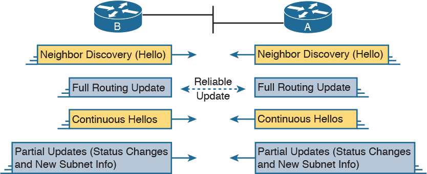
EIGRP does not send full or partial update messages based on a short periodic timer, so EIGRP cannot rely on update messages to monitor the state of EIGRP neighbors. So, using the same basic ideas as OSPF, EIGRP defines a Hello message. The EIGRP Hello message and protocol defines that each router should send a periodic Hello message on each interface, so that all EIGRP routers know that the router is still working. Figure 9-8 shows the idea.

Normally, EIGRP neighbors use the same Hello Interval, which is the time period between each EIGRP Hello. Routers also must receive a Hello from a neighbor within a time called the Hold Interval, with a default setting of three times the Hello Interval.
For instance, imagine both R1 and R2 use default settings of 5 and 15 for their Hello and Hold Intervals. Under normal conditions, R1 receives Hellos from R2 every 5 seconds, well within R1’s Hold Interval (15 seconds) before R1 would consider R2 to have failed. If R2 does fail, R2 no longer sends Hello messages. R1 notices that 15 seconds pass without receiving a Hello from R2, so then R1 can choose new routes that do not use R2 as a next-hop router.
Interestingly, EIGRP does not require two neighboring routers to use the same Hello and Hold intervals, but it makes good sense to use the same Hello and Hold intervals on all routers. Unfortunately, the flexibility to use different settings on neighboring routers makes it possible to prevent the neighbors from working properly, just by the poor choice of Hello and Hold intervals. For instance, if R2 changes its Hello/Hold Intervals to 30/60, respectively, but R1 keeps its Hello/Hold Intervals of 5/15 seconds, R1 will believe R2 has failed on a regular basis. R2 sends Hello messages only every 30 seconds, but R1 expects to receive them within its 15-second Hold Interval.
Summary of Interior Routing Protocol Features
Table 9-2 summarizes the features discussed in this chapter, for RIPv2, EIGRP, and OSPFv2. Following the table, the second major section of this chapter begins, which moves into depth about the specifics of how EIGRP works.

EIGRP Concepts and Operation
EIGRP differs from OSPF in some pretty obvious ways, but in some ways EIGRP acts a lot like OSPF. In fact, EIGRP uses a three-step model similar to OSPF when a router first joins a network. These steps each lead to a list or table: the neighbor table, the topology table, and the routing table. All these processes and tables lead toward building the IPv4 routes in the routing table, as follows:
1. Neighbor discovery: EIGRP routers send Hello messages to discover potential neighboring EIGRP routers and perform basic parameter checks to determine which routers should become neighbors. Neighbors that pass all parameter checks are added to the EIGRP neighbor table.
2. Topology exchange: Neighbors exchange full topology updates when the neighbor relationship comes up, and then only partial updates as needed based on changes to the network topology. The data learned in these updates is added to the router’s EIGRP topology table.
3. Choosing routes: Each router analyzes its respective EIGRP topology tables, choosing the lowest-metric route to reach each subnet. EIGRP places the route with the best metric for each destination into the IPv4 routing table.
This second major section of this chapter discusses the particulars of how EIGRP goes about building its routing table, using these three steps. Although the overall three-step process looks similar to OSPF, the details differ greatly, especially those related to how OSPF uses LS logic to process topology data, whereas EIGRP does not. Also, in addition to these three steps, this section explains some unique logic EIGRP uses when converging and reacting to changes in an internetwork—logic that is not seen with the other types of routing protocols.
EIGRP Neighbors
From the perspective of one router, an EIGRP neighbor is another EIGRP-speaking router, connected to a common subnet, with which the first router is willing to exchange EIGRP topology information. EIGRP uses EIGRP Hello messages to dynamically discover potential neighbors, sending those updates to multicast address 224.0.0.10.
Once another EIGRP router is discovered using Hello messages, routers must perform some basic checking of each potential neighbor before that router becomes an EIGRP neighbor. (A potential neighbor is a router from which an EIGRP Hello has been received.) Then the router checks the following settings to determine whether the router should be allowed to be a neighbor:
![]() It must pass the authentication process if used.
It must pass the authentication process if used.
![]() It must use the same configured autonomous system number (which is a configuration setting).
It must use the same configured autonomous system number (which is a configuration setting).
![]() The source IP address used by the neighbor’s Hello must be in the same subnet as the local router’s interface IP address/mask.
The source IP address used by the neighbor’s Hello must be in the same subnet as the local router’s interface IP address/mask.
![]() The routers' EIGRP K-values must match. (However, Cisco recommends to not change these values.)
The routers' EIGRP K-values must match. (However, Cisco recommends to not change these values.)
EIGRP uses relatively straightforward verification checks for neighbors. First, if authentication is configured, the two routers must be using the same type of authentication and the same authentication key (password). Second, EIGRP configuration includes a parameter called an autonomous system number (ASN), which must be the same on two neighboring routers. Finally, the IP addresses used to send the EIGRP Hello messages—the routers’ respective interface IP addresses—must be in the range of addresses on the other routers’ respective connected subnet.
Once two EIGRP routers become neighbors, the routers use the neighbor relationship in much simpler ways as compared to OSPF. Whereas OSPF neighbors have several interim states and a few stable states, EIGRP simply moves to a working state as soon as the neighbor passes the basic verification checks. At that point, the two routers can begin exchanging topology information using EIGRP update messages.
Exchanging EIGRP Topology Information
EIGRP uses EIGRP update messages to send topology information to neighbors. These update messages can be sent to multicast IP address 224.0.0.10 if the sending router needs to update multiple routers on the same subnet; otherwise, the updates are sent to the unicast IP address of the particular neighbor. (Hello messages are always sent to the 224.0.0.10 multicast address.) The use of multicast packets on LANs allows EIGRP to exchange routing information with all neighbors on the LAN efficiently.
EIGRP sends update messages without UDP or TCP, but it does use a protocol called Reliable Transport Protocol (RTP). RTP provides a mechanism to resend any EIGRP messages that are not received by a neighbor. By using RTP, EIGRP can better avoid loops because a router knows for sure that the neighboring router has received any updated routing information. (The use of RTP is just another example of a difference between basic DV protocols like RIP, which have no mechanism to know whether neighbors receive update messages, and the more advanced EIGRP.)
Note
The acronym RTP also refers to a different protocol, Real-time Transport Protocol (RTP), which is used to transmit voice and video IP packets.
EIGRP neighbors use both full routing updates and partial updates. A full update means that a router sends information about all known routes, whereas a partial update includes only information about recently changed routes. Full updates occur when neighbors first come up. After that, the neighbors send only partial updates in reaction to changes to a route.
Figure 9-9 summarizes many of the details discussed so far in this section, from top to bottom. It first shows neighbor discovery with Hellos, the sending of full updates, the maintenance of the neighbor relationship with ongoing Hellos, and partial updates.
Note that EIGRP refers to the information exchanged in the updates as topology information. The information is not nearly as detailed as OSPF LS topology data, and it does not attempt to describe every router and link in the network. However, it does describe more than just a distance (metric) and vector (next-hop router) for the local router—a local router also learns the metric as used by the next-hop router. This added information is used to help EIGRP converge quickly, without causing loops, as discussed in the upcoming section “EIGRP Convergence.”
Calculating the Best Routes for the Routing Table
EIGRP calculates the metric for routes much differently than any other routing protocol. For instance, with OSPF, anyone with a network diagram and knowledge of the configured OSPF interface costs can calculate the exact OSPF metric (cost) for each route. EIGRP uses a math equation and a composite metric, making the exact metric value hard to predict.
The EIGRP Metric Calculation
The EIGRP composite metric means that EIGRP feeds multiple inputs (called metric components) into the math equation. By default, EIGRP feeds two metric components into the calculation: bandwidth and delay. The result of the calculation is an integer value and is the composite metric for that router.
Note that EIGRP includes other options for how it could calculate the metric, but those options are not normally used. EIGRP supports also using the interface load and interface reliability in the metric calculation. EIGRP also advertises the maximum transmission unit (MTU) associated with the route—that is, the longest IP packet allowed over the route—but does not support using the MTU when calculating the metric. For this book’s purposes, EIGRP uses the default settings, calculating the composite metric based on the bandwidth and delay.
EIGRP’s metric calculation formula actually helps describe some of the key points about the composite metric. (In real life, you seldom if ever need to sit down and calculate what a router will calculate with this formula.) The formula, assuming that the default settings that tell the router to use just bandwidth and delay, is as follows:

In this formula, the term least-bandwidth represents the lowest-bandwidth link in the route, using a unit of kilobits per second. For instance, if the slowest link in a route is a 10-Mbps Ethernet link, the first part of the formula is 107 / 104, which equals 1000. You use 104 in the formula because 10 Mbps is equal to 10,000 Kbps (104 Kbps).
The cumulative-delay value used in the formula is the sum of all the delay values for all outgoing interfaces in the route, with a unit of “tens of microseconds.”
Using these two inputs helps EIGRP pick the best route with a little more balance than does OSPF. Using the least bandwidth lets EIGRP avoid routes with the slowest individual links, which are usually the links with the most congestion. At the same time, the delay part of the equation adds the delay for every link, so that routes with a large number of links will be relatively less desirable than a route with fewer links.
You can set both bandwidth and delay for each link, using the cleverly named bandwidth and delay interface subcommands.
Note
Most show commands, including show ip eigrp topology and show interfaces, list delay settings as the number of microseconds of delay. Note that the EIGRP metric formula uses a unit of tens of microseconds.
An Example of Calculated EIGRP Metrics
Now that you have an idea of how the router’s EIGRP math works, next consider an example that connects what a router learns in an EIGRP update message, local configuration settings, and the calculation of the metric for a single route.
To calculate the metric, a local router must consider the information received from the neighboring router as well as its local interface settings. First, EIGRP update messages list the subnet number and mask, along with all the metric components: the cumulative delay, minimum bandwidth, along with the other usually unused metric components. The local router then considers the bandwidth and delay settings on the interface on which the update was received, and calculates a new metric.
For example, Figure 9-10 shows Router R1 learning about subnet 10.1.3.0/24 from Router R2. The EIGRP update message from R2 lists a minimum bandwidth of 100,000 Kbps, and a cumulative delay of 100 microseconds. R1’s S0/1 interface has an interface bandwidth set to 1544 Kbps—the default bandwidth on a serial link—and a delay of 20,000 microseconds.

Next, consider how R1 thinks about the least-bandwidth part of the calculation. R1 discovers that its S0/1 interface bandwidth (1544 Kbps, or 1.544 Mbps) is less than the advertised minimum bandwidth of 100,000 Kbps, or 100 Mbps. R1 needs to use this new, slower bandwidth in the metric calculation. (If R1’s S0/1 interface had a bandwidth of 100,000 Kbps or more in this case, R1 would instead use the minimum bandwidth listed in the EIGRP update from R2.)
As for interface delay, the router always adds its interface delay to the delay listed in the EIGRP update. However, the unit for delay can be a bit of a challenge. The units, and their use, are as follows:
Unit of microseconds: Listed in the output of show commands such as show interfaces and show ip eigrp topology, and in the EIGRP update messages
Unit of tens-of-microseconds: Used by the interface mode configuration command (delay), with which to set the delay, and in the EIGRP metric calculation
Because of this weird difference in units, when looking at the delay, make sure you keep the units straight. In this particular example:
![]() R1 received an update that lists delay of 100 (microseconds), which R1 converts to the equivalent 10 tens of microseconds before using it in the formula.
R1 received an update that lists delay of 100 (microseconds), which R1 converts to the equivalent 10 tens of microseconds before using it in the formula.
![]() R1 sees its S0/1 interface setting of 20,000 microseconds, which equals 2000 tens of microseconds
R1 sees its S0/1 interface setting of 20,000 microseconds, which equals 2000 tens of microseconds
![]() For the purposes of the calculation, R1 adds 10 tens of microseconds from the update message to 2000 tens of microseconds for the interface for a total delay of 2010 tens of microseconds.
For the purposes of the calculation, R1 adds 10 tens of microseconds from the update message to 2000 tens of microseconds for the interface for a total delay of 2010 tens of microseconds.
This example results in the following metric calculation:

Note
For those of you who repeat this math at home, IOS rounds down the division in this formula to the nearest integer before performing the rest of the formula. In this case, 107 / 1544 is rounded down to 6476, before adding the 2010 and then multiplying by 256.
If multiple possible routes to subnet 10.1.3.0/24 exist, Router R1 also calculates the metric for those routes and chooses the route with the best (lowest) metric to be added to the routing table.
Note
The examples in this chapter show routers with Gigabit interfaces, which default their delay settings to 10 microseconds. However, IOS adjusts the delay based on the actual speed of a LAN interface. In the examples in this chapter and the next, all the LAN interfaces happen to be running at 100 Mbps, making the delay be 100 microseconds.
Caveats with Bandwidth on Serial Links
EIGRP’s robust metric gives it the ability to choose routes that include more router hops but with faster links. However, to ensure that the right routes are chosen, engineers must take care to configure meaningful bandwidth and delay settings. In particular, serial links default to a bandwidth of 1544 and a delay of 20,000 microseconds, as used in the example shown in Figure 9-10. However, IOS cannot automatically change the bandwidth and delay settings based on the Layer 1 speed of a serial link. So, using default bandwidth and delay settings, particularly the bandwidth setting on serial links, can lead to problems.
Figure 9-11 shows the problem with using default bandwidth settings and how EIGRP uses the better (faster) route when the bandwidth is set correctly. The figure focuses on router B’s route to subnet 10.1.1.0/24 in each case. In the left side of the figure, all serial interfaces use defaults, even though the top serial link actually runs at a slow 64 Kbps. The right side of the figure shows the results when the slow serial link’s bandwidth command is changed to reflect the correct (slow) speed.

Generally, a good metric strategy for networks that use EIGRP is to set the WAN bandwidth to match the actual Layer 1 speed, use defaults for LAN interfaces, and EIGRP will usually choose the best routes.
EIGRP Convergence
Now that you have seen the details of how EIGRP forms neighbor relationships, exchanges routing information, and calculates the best route, the rest of this section looks at the most interesting part of EIGRP: EIGRP’s work to converge to a new loop-free route.
Loop avoidance poses one of the most difficult problems with any dynamic routing protocol. DV protocols overcome this problem with a variety of tools, some of which create a large portion of the minutes-long convergence time after a link failure. LS protocols overcome this problem by having each router keep a full topology of the network, so by running a rather involved mathematical model (for example, OSPF’s SPF algorithm), a router can avoid any loops.
EIGRP avoids loops by keeping some basic topological information, while keeping much less information as compared to LS protocols like OSPF. EIGRP keeps a record of each possible next-hop router for alternate routes, and some metric details related to those routes, but no information about the topology beyond the next-hop routers. This sparser topology information does not require the sophisticated Shortest Path First (SPF) algorithm, but it does allow quick convergence to loop-free routes.
Feasible Distance and Reported Distance
First, before getting into how EIGRP converges, you need to know a few additional EIGRP terms. With EIGRP, a local router needs to consider its own calculated metric for each route, but at the same time, the local router considers the next-hop router’s calculated metric for that same destination subnet. And EIGRP has special terms for those metrics, as follows:
![]() Feasible distance (FD): The local router’s composite metric of the best route to reach a subnet, as calculated on the local router
Feasible distance (FD): The local router’s composite metric of the best route to reach a subnet, as calculated on the local router
![]() Reported distance (RD): The next-hop router’s best composite metric for that same subnet
Reported distance (RD): The next-hop router’s best composite metric for that same subnet
As usual, the definition makes more sense with an example. Using the same advertisement as earlier in Figure 9-10, Figure 9-12 shows the two calculations done by R1. One calculation finds R1’s own metric (FD) for its one route for subnet 10.1.3.0/24, as discussed around Figure 9-10. The other uses the metric components in the update received from R2, to calculate what R2 would have calculated for R2’s metric to reach this same subnet. R1’s second calculation based on R2’s information—a slowest bandwidth of 100,000 Kbps and a cumulative delay of 100 microseconds—is R1’s RD for this route.

Following the steps in the figure:
1. R2 calculates its own metric (its FD) for R2’s route for 10.1.3.0/24, based on a bandwidth of 100,000 Kbps and a delay of 100 microseconds.
2. R2 sends the EIGRP update that lists 10.1.3.0/24, with these same metric components.
3. R1 calculates the RD for this route, using the same math R2 used at Step 1, using the information in the update message from Step 2.
4. R1 calculates its own metric, from R1’s perspective, by considering the bandwidth and delay of R1’s S0/1 interface, as discussed earlier around Figure 9-10.
In fact, based on the information in Figure 9-12, R2’s FD to reach subnet 10.1.3.0/24, which is also R1’s RD to reach 10.1.3.0/24, could be easily calculated:

At this point, R1 knows its own calculated metric for the route, called the FD, and R1 knows next-hop Router R2’s metric for R2’s route to that same subnet. R1 calls that R2’s RD.
Now that you have a general idea about the FD and RD concept, consider the EIGRP convergence process. EIGRP convergence has two branches in its logic, based on whether the failed route does or does not have a feasible successor route. The decision of whether a router has a feasible successor route depends on the FD and RD values of the competing routes to reach a given subnet. The next topic defines this concept of a feasible successor route and discusses what happens in that case.
EIGRP Successors and Feasible Successors
EIGRP calculates the metric for each route to reach each subnet. For a particular subnet, the route with the best metric is called the successor, with the router filling the IP routing table with this successor route. (This successor route’s metric is called the feasible distance, as introduced earlier.)
Of the other routes to reach that same subnet—routes whose metrics were larger than the FD for the successor route—EIGRP needs to determine which alternate route can be used immediately if the currently best route fails, without causing a routing loop. EIGRP runs a simple algorithm to identify which routes could be used, keeping these loop-free backup routes in its topology table and using them if the currently best route fails. These alternative, immediately usable routes are called feasible successor routes because they can feasibly be used as the new successor route when the previous successor route fails.
A router determines whether a route is a feasible successor based on the feasibility condition:
If a nonsuccessor route’s RD is less than the FD, the route is a feasible successor route.
Although it is technically correct, this definition is much more understandable with an example. Figure 9-13 begins an example in which router E chooses its best route to subnet 1. Router E learns three routes to subnet 1, with next-hop routers B, C, and D. The figure shows the metrics as calculated on router E, as listed in router E’s EIGRP topology table. Router E finds that the route through router D has the lowest metric, making that router E’s successor route for subnet 1. Router E adds that route to its routing table, as shown. The FD is the metric calculated for this route, a value of 14,000 in this case.

At the same time, EIGRP on router E decides whether either of the other two routes to subnet 1 can be used immediately if the route through router D fails for whatever reason. Only a feasible successor route can be used. To meet the feasibility condition, the alternate route’s RD must be less than the FD of the successor route.
Figure 9-14 demonstrates that one of the two other routes meets the feasibility condition and is therefore a feasible successor route. The figure shows an updated version of Figure 9-13. Router E uses the following logic to determine that the route through router B is not a feasible successor route, but the route through router C is, as follows:
![]() Router E compares the FD of 14,000 to the RD of the route through router B (15,000). Router B’s RD is worse than router E’s FD, so this route is not a feasible successor.
Router E compares the FD of 14,000 to the RD of the route through router B (15,000). Router B’s RD is worse than router E’s FD, so this route is not a feasible successor.
![]() Router E compares the FD of 14,000 to the RD of the route through router C (13,000). Router C’s RD is better than router E’s FD, making this route a feasible successor.
Router E compares the FD of 14,000 to the RD of the route through router C (13,000). Router C’s RD is better than router E’s FD, making this route a feasible successor.

If the route to subnet 1 through router D fails, router E can immediately put the route through router C into the routing table without fear of creating a loop. Convergence occurs almost instantly in this case.
The Query and Reply Process
When a route fails, and the route has no feasible successor, EIGRP uses a distributed algorithm called Diffusing Update Algorithm (DUAL) to choose a replacement route. DUAL sends queries looking for a loop-free route to the subnet in question. When the new route is found, DUAL adds it to the routing table.
The EIGRP DUAL process simply uses messages to confirm that a route exists, and would not create a loop, before deciding to replace a failed route with an alternative route. For instance, in Figure 9-14, imagine that both routers C and D fail. Router E does not have any remaining feasible successor route for subnet 1, but there is an obvious physically available path through router B. To use the route, router E sends EIGRP query messages to its working neighbors (in this case, router B). Router B’s route to subnet 1 is still working fine, so router B replies to router E with an EIGRP reply message, simply stating the details of the working route to subnet 1 and confirming that it is still viable. Router E can then add a new route to subnet 1 to its routing table, without fear of a loop.
Replacing a failed route with a feasible successor takes a very short amount of time, usually less than a second or two. When queries and replies are required, convergence can take slightly longer, but in most networks, convergence can still occur in less than 10 seconds.
Chapter Review
One key to doing well on the exams is to perform repetitive spaced review sessions. Review this chapter’s material using either the tools in the book, DVD, or interactive tools for the same material found on the book’s companion website. Refer to the “Your Study Plan” element for more details. Table 9-3 outlines the key review elements and where you can find them. To better track your study progress, record when you completed these activities in the second column.

