Chapter 1: An Introduction to Query Tuning and Optimization

We have all been there; suddenly, you get a phone call notifying you of an application outage and asking you to urgently join a conference bridge. After joining the call, you are told that the application is so slow that the company is not able to conduct business; it is losing money and, potentially, customers too. And many times, nobody on the call can provide any additional information that can help you find out what the problem is. So, what you should do? Where do you start? And perhaps more important, how do you avoid these problems from reoccurring in the future?

Although an outage can occur for several different reasons, including a hardware failure or an operating system problem, as a database professional, you should be able to proactively tune and optimize your databases and be ready to quickly troubleshoot any problem that may eventually occur. This book will provide you with the knowledge and tools required to do just that. By focusing on SQL Server performance, and more specifically on query tuning and optimization, this book can help you, first, to avoid these performance problems by optimizing your databases and, second, to quickly troubleshoot and fix them if they happen to appear.

One of the best ways to learn how to improve the performance of your databases is not only to work with the technology, but to understand how the technology works, what it can do for you, how to get the most benefit out of it, and even what its limitations are. The most important SQL Server component that impacts the performance of your queries is the SQL Server query processor, which includes the query optimizer and the execution engine. With a perfect query optimizer, you could just submit any query and you would get a perfect execution plan every time. And with a perfect execution engine, each of your queries would run in just a matter of milliseconds. But the reality is that query optimization is a very complex problem, and no query optimizer can find the best plan all the time – at least, not in a reasonable amount of time. For complex queries, there are so many possible execution plans a query optimizer would need to analyze. And even supposing that a query optimizer could analyze all the possible solutions, the next challenge would be to decide which plan to choose. Which one is the most efficient? Choosing the best plan would require estimating the cost of each solution, which, again, is a very complicated task.

Don’t get me wrong: the SQL Server query optimizer does an amazing job and gives you a good execution plan almost all the time. But you still need to understand which information you need to provide to the query optimizer so that it can do a good job, which may include providing the right indexes and adequate statistics, as well as defining the required constraints and a good database design. SQL Server even provides you with tools to help you in some of these areas, including the Database Engine Tuning Advisor (DTA) and the auto-create and auto-update statistics features. But there is still more you can do to improve the performance of your databases, especially when you are building high-performance applications. Finally, you need to understand the cases where the query optimizer may not give you a good execution plan and what to do in those cases.

So, for you to better understand this technology, this chapter will start by providing you with an overview of how the SQL Server query processor works and introducing the concepts that will be covered in more detail in the rest of the book. We will explain the purpose of both the query optimizer and the execution engine and how they may interact with the plan cache so that you can reuse plans as much as possible. Finally, we will learn how to work with execution plans, which are the primary tools we’ll use to interact with the query processor.

We will cover the following topics in this chapter:

• Query processor architecture
• Analyzing execution plans
• Getting plans from a trace or the plan cache
• SET STATISTICS TIME and IO statements

Query Processor Architecture

At the core of the SQL Server database engine are two major components:

• The storage engine: The storage engine is responsible for reading data between the disk and memory in a manner that optimizes concurrency while maintaining data integrity.
• The relational engine (also called the query processor): The query processor, as the name suggests, accepts all queries submitted to SQL Server, devises a plan for their optimal execution, and then executes the plan and delivers the required results.

Queries are submitted to SQL Server using SQL or Structured Query Language (or T-SQL, the Microsoft SQL Server extension to SQL). Because SQL is a high-level declarative language, it only defines what data to get from the database, not the steps required to retrieve that data or any of the algorithms for processing the request. Thus, for each query it receives, the first job of the query processor is to devise, as quickly as possible, a plan that describes the best possible way (or, at the very least, an efficient way) to execute the query. Its second job is to execute the query according to that plan. Each of these tasks is delegated to a separate component within the query processor. The query optimizer devises the plan and then passes it along to the execution engine, which will execute the plan and get the results from the database.

The SQL Server query optimizer is cost-based. It analyzes several candidate execution plans for a given query, estimates the cost of each of these plans, and selects the plan with the lowest cost of the choices considered. Given that the query optimizer cannot consider every possible plan for every query, it must find a balance between the optimization time and the quality of the selected plan.

Therefore, the query optimizer is the SQL Server component that has the biggest impact on the performance of your databases. After all, selecting the right or wrong execution plan could mean the difference between a query execution time of milliseconds and one that takes minutes or even hours. Naturally, a better understanding of how the query optimizer works can help both database administrators and developers write better queries and provide the query optimizer with the information it needs to produce efficient execution plans. This book will demonstrate how you can use your newfound knowledge of the query optimizer’s inner workings; in addition, it will give you the knowledge and tools to troubleshoot the cases when the query optimizer is not giving you a good execution plan.

To arrive at what it believes to be the best plan for executing a query, the query processor performs several different steps; the entire query-processing process is shown in the following diagram:

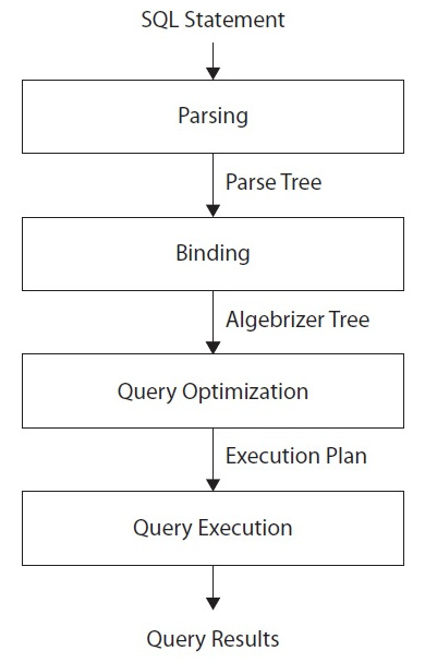
Figure 1.1 – Query processing phases

We will look at this process in more detail in Chapter 3, The Query Optimizer, but let’s just run through the steps briefly now:

1. Parsing and binding: The query is parsed and bound. Assuming the query is valid, the output of this phase is a logical tree, with each node in the tree representing a logical operation that the query must perform, such as reading a particular table or performing an inner join.
2. Query optimization: The logical tree is then used to run the query optimization process, which roughly consists of the following two steps:
   1. Generating possible execution plans: Using the generated logical tree, the query optimizer devises several possible ways to execute the query (that is, several possible execution plans). An execution plan is, in essence, a set of physical operations (such as an Index Seek or a Nested Loop Join) that can be performed to produce the required result, as described by the logical tree.
   2. Assessing the cost of each plan: Although the query optimizer does not generate every possible execution plan, it assesses the resource and time cost of each generated plan (or, more exactly, every considered operation). The plan that the query optimizer deems to have the lowest cost is selected and then passed along to the execution engine.
3. Query execution and plan caching: The query is executed by the execution engine according to the selected plan; the plan may be stored in memory in the plan cache.

Although the query optimization process will be explained in greater detail in Chapter 3, The Query Optimizer, let’s expand a little bit.

Parsing and binding

Parsing and binding are the first operations that are performed when a query is submitted to a SQL Server instance. Parsing makes sure that the T-SQL query has valid syntax and that it translates the SQL query into an initial tree representation: specifically, a tree of logical operators representing the high-level steps required to execute the query in question. Initially, these logical operators will be closely related to the original syntax of the query and will include such logical operations as get data from the Customer table, get data from the Contact table, perform an inner join, and so on. Different tree representations of the query will be used throughout the optimization process, and the logical tree will receive different names until it is finally used to initialize the Memo structure during the optimization process.

Binding is mostly concerned with name resolution. During the binding operation, SQL Server makes sure that all the object names do exist, and it associates every table and column name on the parse tree with its corresponding object in the system catalog. The output of this second process is called an algebrizer tree, which is then sent to the query optimizer to be optimized.

Query optimization

The next step is the optimization process, which involves generating candidate execution plans and selecting the best of these plans according to their cost. As mentioned previously, the SQL Server query optimizer uses a cost-estimation model to estimate the cost of each of the candidate plans.

Query optimization could be also seen, in a simplistic way, as the process of mapping the logical query operations expressed in the original tree representation to physical operations, which can be carried out by the execution engine. So, it’s the functionality of the execution engine that is being implemented in the execution plans being created by the query optimizer; that is, the execution engine implements a certain number of different algorithms, and the query optimizer must choose from these algorithms when formulating its execution plans. It does this by translating the original logical operations into the physical operations that the execution engine is capable of performing. Execution plans show both the logical and physical operations of each operator. Some logical operations, such as sorts, translate into the same physical operation, whereas other logical operations map to several possible physical operations. For example, a logical join can be mapped to a Nested Loop Join, Merge Join, or Hash Join physical operator. However, this is not as simple as a one-to-one operator matching and follows a more complicated process, based on transformation rules, which will be explained in more detail in Chapter 3, The Query Optimizer.

Thus, the final product of the query optimization process is an execution plan: a tree consisting of several physical operators, which contain a selection of algorithms to be performed by the execution engine to obtain the desired results from the database.

Generating candidate execution plans

As stated previously, the basic purpose of the query optimizer is to find an efficient execution plan for your query. Even for relatively simple queries, there may be a large number of different ways to access the data to produce the same result. As such, the query optimizer must select the best possible plan from what may be a very large number of candidate execution plans. Making a wise choice is important because the time taken to return the results to the user can vary wildly, depending on which plan is selected.

The job of the query optimizer is to create and assess as many candidate execution plans as possible, within certain criteria, to find a good enough plan, which may be (but is not necessarily) the optimal plan. We define the search space for a given query as the set of all possible execution plans for that query, in which any possible plan in this search space returns the same results. Theoretically, to find the optimum execution plan for a query, a cost-based query optimizer should generate all possible execution plans that exist in that search space and correctly estimate the cost of each plan. However, some complex queries may have thousands, or even millions, of possible execution plans, and although the SQL Server query optimizer can typically consider a large number of candidate execution plans, it cannot perform an exhaustive search of all the possible plans for every query. If it did, the time taken to assess all of the plans would be unacceptably long and could start to have a major impact on the overall query execution time.

The query optimizer must strike a balance between optimization time and plan quality. For example, if the query optimizer spends 100 milliseconds finding a good enough plan that executes in 5 seconds, then it doesn’t make sense to try to find the perfect or most optimal plan if it is going to take 1 minute of optimization time, plus the execution time. So, SQL Server does not do an exhaustive search. Instead, it tries to find a suitably efficient plan as quickly as possible. As the query optimizer is working within a time constraint, there’s a chance that the selected plan may be the optimal plan, but it is also likely that it may just be something close to the optimal plan.

To explore the search space, the query optimizer uses transformation rules and heuristics. Candidate execution plans are generated inside the query optimizer using transformation rules, and the use of heuristics limits the number of choices considered to keep the optimization time reasonable. The set of alternative plans that’s considered by the query optimizer is referred to as the plan space, and these plans are stored in memory during the optimization process in a component called the Memo. Transformation rules, heuristics, and the Memo component’s structure will be discussed in more detail in Chapter 3, The Query Optimizer.

Plan cost evaluation

Searching or enumerating candidate plans is just one part of the optimization process. The query optimizer still needs to estimate the cost of these plans and select the least expensive one. To estimate the cost of a plan, it estimates the cost of each physical operator in that plan, using costing formulas that consider the use of resources such as I/O, CPU, and memory. This cost estimation depends mostly on both the algorithm used by the physical operator and the estimated number of records that will need to be processed. This estimate is known as the cardinality estimation.

To help with this cardinality estimation, SQL Server uses and maintains query optimization statistics, which contain information describing the distribution of values in one or more columns of a table. Once the cost for each operator is estimated using estimations of cardinality and resource demands, the query optimizer will add up all of these costs to estimate the cost for the entire plan. Rather than go into more detail here, we will cover statistics and cost estimation in more detail in Chapter 6, Understanding Statistics.

Query execution and plan caching

Once the query has been optimized, the resulting plan is used by the execution engine to retrieve the desired data. The generated execution plan may be stored in memory in the plan cache so that it can be reused if the same query is executed again. SQL Server has a pool of memory that is used to store both data pages and execution plans, among other objects. Most of this memory is used to store database pages, and it is called the buffer pool. A smaller portion of this memory contains the execution plans for queries that were optimized by the query optimizer and is referred to as the plan cache (previously known as the procedure cache). The percentage of memory that’s allocated to the plan cache or the buffer pool varies dynamically, depending on the state of the system.

Before optimizing a query, SQL Server first checks the plan cache to see if an execution plan exists for the query or, more exactly, a batch, which may consist of one or more queries. Query optimization is a relatively expensive operation, so if a valid plan is available in the plan cache, the optimization process can be skipped and the associated cost of this step, in terms of optimization time, CPU resources, and so on, can be avoided. If a plan for the batch is not found, the batch is compiled to generate an execution plan for all the queries in the stored procedure, the trigger, or the dynamic SQL batch. Query optimization begins by loading all the interesting statistics. Then, the query optimizer validates if the statistics are outdated. For any outdated statistics, when using the statistics default options, it will update the statistics and proceed with the optimization process.

Once a plan has been found in the plan cache or a new one is created, the plan is validated for schema and data statistics changes. Schema changes are verified for plan correctness. Statistics are also verified: the query optimizer checks for new applicable statistics or outdated statistics. If the plan is not valid for any of these reasons, it is discarded, and the batch or individual query is compiled again. Such compilations are known as recompilations. This process is summarized in the following diagram:

Figure 1.2 – Compilation and recompilation process

Query plans may also be removed from the plan cache when SQL Server is under memory pressure or when certain statements are executed. Changing some configuration options (for example, max degree of parallelism) will clear the entire plan cache. Alternatively, some statements, such as changing the database configuration with certain ALTER DATABASE options, will clear all the plans associated with that particular database.

However, it is also worth noting that reusing an existing plan may not always be the best solution for every instance of a given query, and as a result, some performance problems may appear. For example, depending on the data distribution within a table, the optimal execution plan for a query may differ greatly, depending on the parameters being used to get data from such table. More details about these problems, parameter sniffing, and the plan cache, in general, will be covered in greater detail in Chapter 8, Understanding Plan Caching.

Now that we have a foundation for the query processor architecture, let’s learn how to interact with it using execution plans.

Note

Parameter-sensitive plan optimization, a new feature with SQL Server 2022, will also be covered in Chapter 8, Understanding Plan Caching.

Analyzing execution plans

Primarily, we’ll interact with the query processor through execution plans, which, as mentioned earlier, are ultimately trees consisting of several physical operators that, in turn, contain the algorithms to produce the required results from the database. Given that we will make extensive use of execution plans throughout this book, in this section, we will learn how to display and read them.

You can request either an actual or an estimated execution plan for a given query, and either of these two types can be displayed as a graphic, text, or XML plan. Any of these three formats show the same execution plan – the only difference is how they are displayed and the level of detail they contain.

When an estimated plan is requested, the query is not executed; the plan that’s displayed is simply the plan that SQL Server would most probably use if the query were executed, bearing in mind that a recompile, which we’ll discuss later, may generate a different plan at execution time. However, when an actual plan is requested, you need to execute the query so that the plan is displayed along with the query results. Nevertheless, using an estimated plan has several benefits, including displaying a plan for a long-running query for inspection without actually running the query, or displaying a plan for update operations without changing the database.

Note

Starting with SQL Server 2014 but using SQL Server Management Studio 2016 (version 13 or later), you can also use Live Query Statistics to view the live execution plan of an active query. Live Query Statistics will be covered in Chapter 9, The Query Store.

Graphical plans

You can display graphical plans in SQL Server Management Studio by clicking the Display Estimated Execution Plan button or the Include Actual Execution Plan button from the SQL Editor toolbar. Clicking Display Estimated Execution Plan will show the plan immediately, without executing the query. To request an actual execution plan, you need to click Include Actual Execution Plan and then execute the query and click the Execution plan tab.

As an example, copy the following query to Management Studio Query Editor, select the AdventureWorks2019 database, click the Include Actual Execution Plan button, and execute the following query:

SELECT DISTINCT(City) FROM Person.Address

Then, select the Execution Plan tab in the results pane. This will display the plan shown here:

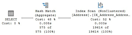
Figure 1.3 – Graphical execution plan

Note

This book contains a large number of sample SQL queries, all of which are based on the AdventureWorks2019 database, although Chapter 11, An Introduction to Data Warehouses, additionally uses the AdventureWorksDW2019 database. All code has been tested on SQL Server 2022 CTP (community technology preview) 2.0. Note that these sample databases are not included in your SQL Server installation but instead can be downloaded from https://docs.microsoft.com/en-us/sql/samples/adventureworks-install-configure. You need to download the family of sample databases for SQL Server 2019.

Note

Although you could run the examples in this book using any recent version of SQL Server Management Studio, it is strongly recommended to use version 19.0 or later to work with SQL Server 2022. Although SQL Server Management Studio is not available on a SQL Server installation and must be downloaded separately, every SQL Server version requires a specific version of SQL Server Management Studio. For example, v19.0 must be added, among other things, if you wish to support Contained Always On Availability Groups or the latest showplan XML schema. This book uses SQL Server Management Studio v19.0 Preview 2.

Each node in the tree structure is represented as an icon that specifies a logical and physical operator, such as the Index Scan and the Hash Aggregate operators, as shown in Figure 1.3. The first icon is a language element called the Result operator, which represents the SELECT statement and is usually the root element in the plan.

Operators implement a basic function or operation of the execution engine; for example, a logical join operation could be implemented by any of three different physical join operators: Nested Loop Join, Merge Join, or Hash Join. Many more operators are implemented in the execution engine. You can find the entire list at http://msdn.microsoft.com/en-us/library/ms191158(v=sql.110).aspx.

The query optimizer builds an execution plan and chooses which operations may read records from the database, such as the Index Scan operator shown in the previous plan. Alternatively, it may read records from another operator, such as the Hash Aggregate operator, which reads records from the Index Scan operator.

Each node in the plan is related to a parent node, connected with arrowheads, where data flows from a child operator to a parent operator and the arrow width is proportional to the number of rows. After the operator performs some function on the records it has read, the results are output to its parent. You can hover your mouse pointer over an arrow to get more information about that data flow, which is displayed as a tooltip. For example, if you hover your mouse pointer over the arrow between the Index Scan and Hash Aggregate operators, shown in Figure 1.3, you will get the data flow information between these operators, as shown here:

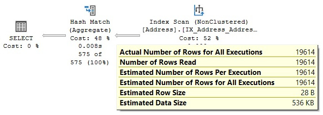
Figure 1.4 – Data flow between the Index Scan and Hash Aggregate operators

By looking at the actual number of rows, you can see that the Index Scan operator is reading 19,614 rows from the database and sending them to the Hash Aggregate operator. The Hash Aggregate operator is, in turn, performing some operation on this data and sending 575 records to its parent, which you can also see by placing your mouse pointer over the arrow between the Hash Aggregate operator and the SELECT icon.

Basically, in this plan, the Index Scan operator is reading all 19,614 rows from an index, and the Hash Aggregate operator is processing these rows to obtain the list of distinct cities, of which there are 575, which will be displayed in the Results window in Management Studio. Also, notice how you can see the estimated number of rows, which is the query optimizer’s cardinality estimation for this operator, as well as the actual number of rows. Comparing the actual and the estimated number of rows can help you detect cardinality estimation errors, which can affect the quality of your execution plans, as will be discussed in Chapter 6, Understanding Statistics.

To perform their job, physical operators implement at least the following three methods:

• Open() causes an operator to be initialized and may include setting up any required data structures.
• GetRow() requests a row from the operator.
• Close() performs some cleanup operations and shuts down the operator once it has performed its role.

An operator requests rows from other operators by calling its GetRow() method, which also means that execution in a plan starts from left to right. Because GetRow() produces just one row at a time, the actual number of rows that’s displayed in the execution plan is also the number of times the method was called on a specific operator, plus an additional call to GetRow(), which is used by the operator to indicate the end of the result set. In the previous example, the Hash Aggregate operator calls the Open() method once, the GetRow() operator 19,615 times, and the Close() operator once on the Index Scan operator.

Note

For now, and for most of this book, we will be explaining the traditional query-processing mode in which operators process only one row at a time. This processing mode has been used in all versions of SQL Server, at least since SQL Server 7.0, when the current query optimizer was built and released. Later, in Chapter 11, An Introduction to Data Warehouses, we will touch on the new batch-processing mode, introduced with SQL Server 2012, in which operators process multiple rows at a time and it is used by operators related to the columnstore indexes.

In addition to learning more about the data flow, you can also hover your mouse pointer over an operator to get more information about it. For example, the following screenshot shows information about the Index Scan operator; notice that it includes, among other things, a description of the operator and data on estimated costing information, such as the estimated I/O, CPU, operator, and subtree costs:

Figure 1.5 – Tooltip for the Index Scan operator

Some of these properties are explained in the following table; others will be explained later in this book:

Table 1.1 – Operator properties

Note

It is worth mentioning that the cost included in these operations is just internal cost units that are not meant to be interpreted in other units, such as seconds or milliseconds. Chapter 3, The Query Optimizer, explains the origin of these cost units.

You can also see the relative cost of each operator in the plan as a percentage of the overall plan, as shown previously in Figure 1.3. For example, the cost of the Index Scan operator is 52 percent of the cost of the entire plan. Additional information from an operator or the entire query can be obtained by using the Properties window. So, for example, choosing the SELECT icon and selecting the Properties window from the View menu (or pressing F4) will show some properties for the entire query, as shown in the following screenshot:

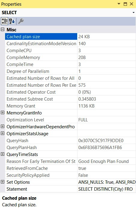
Figure 1.6 – The Properties window for the query

The following table lists the most important properties of a plan, most of which are shown in the preceding screenshot. Some other properties may be available, depending on the query (for example, Parameter List, MissingIndexes, or Warnings):

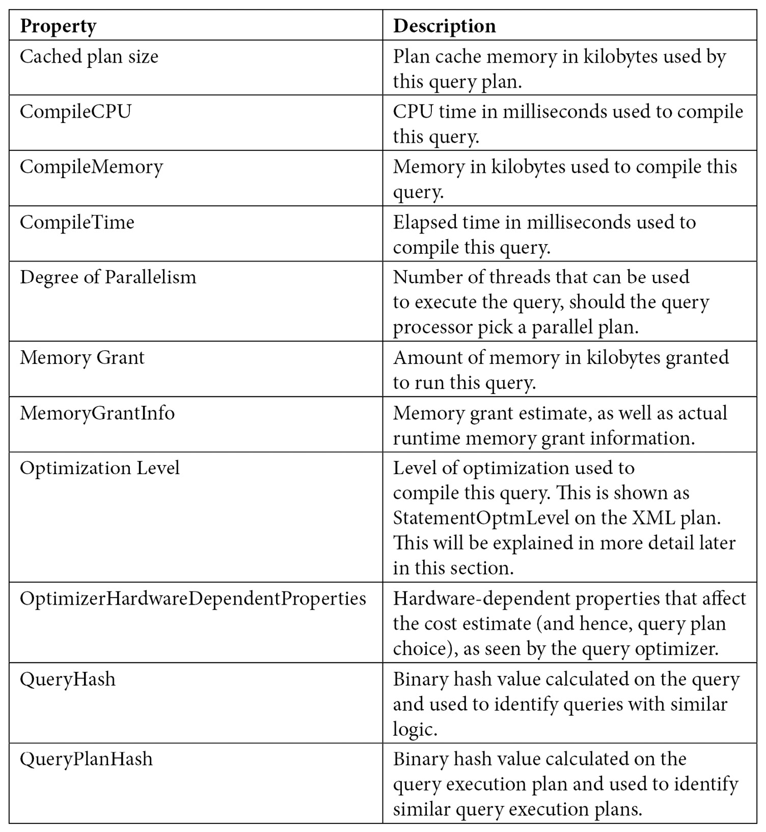
Table 1.2 – Query properties

XML plans

Once you have displayed a graphical plan, you can also easily display it in XML format. Simply right-click anywhere on the execution plan window to display a pop-up menu, as shown in Figure 1.7, and select Show Execution Plan XML…. This will open the XML editor and display the XML plan. As you can see, you can easily switch between a graphical and an XML plan.

If needed, you can save graphical plans to a file by selecting Save Execution Plan As… from the pop-up menu shown in Figure 1.6. The plan, usually saved with a .sqlplan extension, is an XML document containing the XML plan but can be read by Management Studio into a graphical plan. You can load this file again by selecting File and then Open in Management Studio to immediately display it as a graphical plan, which will behave exactly as it did previously. XML plans can also be used with the USEPLAN query hint, which will be explained in Chapter 12, Understanding Query Hints:

Figure 1.7 – Pop-up menu on the execution plan window

The following table shows the different statements you can use to obtain an estimated or actual execution plan in text, graphic, or XML format:

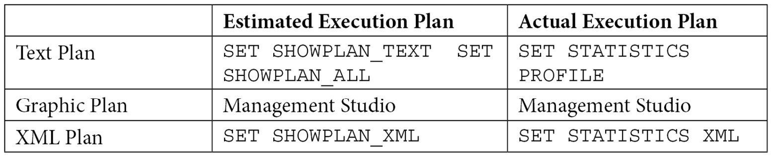
Table 1.3 – Statements for displaying query plans

NOTE

When you run any of the statements listed in the preceding screenshot using the ON clause, it will apply to all subsequent statements until the option is manually set to OFF again.

To show an XML plan, you can use the following commands:

SET SHOWPLAN_XML ON

GO

SELECT DISTINCT(City) FROM Person.Address

GO

SET SHOWPLAN_XML OFF

This will display a single-row, single-column (titled Microsoft SQL Server 2005 XML Showplan) result set containing the XML data that starts with the following:

<ShowPlanXML xmlns="http://schemas.microsoft.com/sqlserver/2004 ...

Clicking the link will show you a graphical plan. Then, you can display the XML plan by following the same procedure explained earlier.

You can browse the basic structure of an XML plan via the following exercise. A very simple query can create the basic XML structure, but in this example, we will see a query that can provide two additional parts: the missing indexes and parameter list elements. Run the following query and request an XML plan:

SELECT * FROM Sales.SalesOrderDetail

WHERE OrderQty = 1

Collapse <MissingIndexes>, <OptimizerStatsUsage>, <RelOp>, <WaisStats>, and <ParameterList> by clicking the minus sign (-) on the left so that you can easily see the entire structure. You should see something similar to the following:

Figure 1.8 – XML execution plan

As you can see, the main components of the XML plan are the <StmtSimple>, <StatementSetOptions>, and <QueryPlan> elements. These three elements include several attributes, some of which were already explained when we discussed the graphical plan. In addition, the <QueryPlan> element also includes other elements, such as <MissingIndexes>, <MemoryGrantInfo>, <OptimizerHardwareDependentProperties>, <RelOp>, <ParameterList>, and others not shown in Figure 1.8, such as <Warnings>, which will be also discussed later in this section. <StmtSimple> shows the following for this example:

<StmtSimple StatementCompId="1" StatementEstRows="68089" StatementId="1"

StatementOptmLevel="FULL" CardinalityEstimationModelVersion="70"

StatementSubTreeCost="1.13478" StatementText="SELECT * FROM

[Sales].[SalesOrderDetail] WHERE [OrderQty]=@1" StatementType="SELECT"

QueryHash="0x42CFD97ABC9592DD" QueryPlanHash="0xC5F6C30459CD7C41"

RetrievedFromCache="false">

<QueryPlan> shows the following:

<QueryPlan DegreeOfParallelism="1" CachedPlanSize="32" CompileTime="3"

CompileCPU="3" CompileMemory="264">

As mentioned previously, the attributes of these and other elements were already explained when we discussed the graphical plan. Others will be explained later in this section or in other sections of this book.

Text plans

As shown in Table 1.3, there are two commands to get estimated text plans: SET SHOWPLAN_TEXT and SET SHOWPLAN_ALL. Both statements show the estimated execution plan, but SET SHOWPLAN_ALL shows some additional information, including the estimated number of rows, estimated CPU cost, estimated I/O cost, and estimated operator cost. However, recent versions of the documentation indicate that all text versions of execution plans will be deprecated in a future version of SQL Server, so it is recommended that you use the XML versions instead.

You can use the following code to display a text execution plan:

SET SHOWPLAN_TEXT ON

GO

SELECT DISTINCT(City) FROM Person.Address

GO

SET SHOWPLAN_TEXT OFF

GO

This code will display two result sets, with the first one returning the text of the T-SQL statement. In the second result set, you will see the following text plan (edited to fit the page), which shows the same Hash Aggregate and Index Scan operators displayed earlier in Figure 1.3:

|--Hash Match(Aggregate, HASH:([Person].[Address].[City]), RESIDUAL …

|--Index Scan(OBJECT:([AdventureWorks].[Person].[Address]. [IX_Address …

SET SHOWPLAN_ALL and SET STATISTICS PROFILE can provide more detailed information than SET SHOWPLAN_TEXT. Also, as shown in Table 1.3, you can use SET SHOWPLAN_ALL to get an estimated plan only and SET STATISTICS PROFILE to execute the query. Run the following example:

SET SHOWPLAN_ALL ON

GO

SELECT DISTINCT(City) FROM Person.Address

GO

SET SHOWPLAN_ALL OFF

GO

The output is shown in the following screenshot:

Figure 1.9 – SET SHOWPLAN_ALL output

Because SET STATISTICS PROFILE executes the query, it provides an easy way to look for cardinality estimation problems because you can easily visually compare multiple operators at a time, which could be complicated to do on a graphical or XML plan. Now, run the following code:

SET STATISTICS PROFILE ON

GO

SELECT * FROM Sales.SalesOrderDetail

WHERE OrderQty * UnitPrice > 25000

GO

SET STATISTICS PROFILE OFF

The output is shown in the following screenshot:

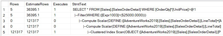
Figure 1.10 – SET STATISTICS PROFILE output

Note that the EstimateRows column was manually moved in Management Studio to be next to the column rows so that you can easily compare the actual against the estimated number of rows. For this particular example, you can see a big difference in cardinality estimation on the Filter operator of 36,395.1 estimated versus five actual rows.

Plan properties

One interesting way to learn about the components of an execution plan, including ones of future versions of SQL Server, is to look at the showplan schema. XML plans comply with a published XSD schema, and you can see the current and older versions of this showplan schema at http://schemas.microsoft.com/sqlserver/2004/07/showplan/. You can also find the address or URL at the beginning of each XML execution plan. At the time of writing, accessing that location on a web browser will show you links where you can access the showplan schemas for all the versions of SQL Server since version 2005 (when XML plans were introduced), as shown in the following screenshot. As you can see, a new showplan schema is introduced with every new release and, in some cases, with a new Service Pack.

The only exception could be SQL Server 2008 R2, which even when it is a new version, shares the same schema as SQL Server 2008. A showplan schema for SQL Server 2022 hasn’t been published at the time of writing:

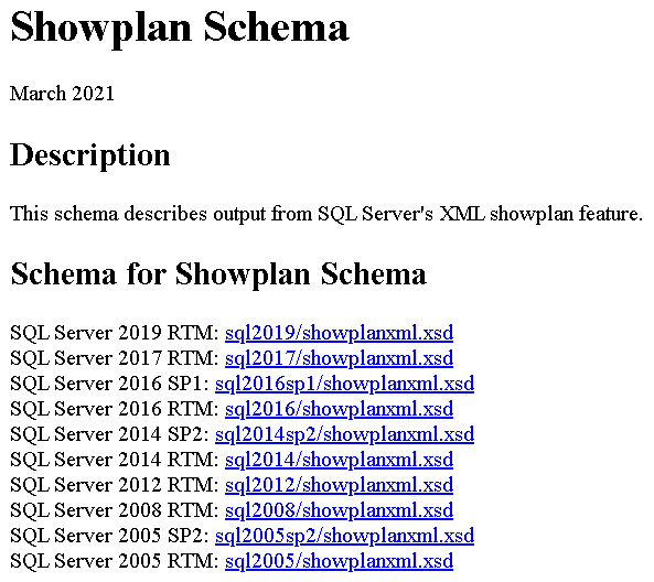
Figure 1.11 – Showplan schema available definitions

Covering all the elements and attributes of an execution plan would take a lot of pages; instead, we will only cover some of the most interesting ones here. Table 1.2 includes descriptions of query properties. We will use this section to describe some of those properties in more detail.

You can see all these properties, as mentioned earlier, by choosing the SELECT icon on a graphical plan and selecting the Properties window from the View menu. An example of the properties of a query was shown earlier in Figure 1.6. The most common operators that are used in execution plans will be covered in more detail in Chapter 4, The Execution Engine.

StatementOptmLevel

Although these attributes refer to concepts that will be explained in more detail later in this book, it’s worth introducing them here. StatementOptmLevel is the query optimization level, which can be either TRIVIAL or FULL. The optimization process may be expensive to initialize and run for very simple queries that don’t require any cost estimation, so to avoid this expensive operation for these simple queries, SQL Server uses the trivial plan optimization. If a query does not apply for a trivial optimization, a full optimization will have to be performed. For example, in SQL Server 2019, the following query will produce a trivial plan:

SELECT * FROM Sales.SalesOrderHeader

WHERE SalesOrderID = 43666

You can use the undocumented (and therefore unsupported) trace flag 8757 to test the behavior if you want to disable the trivial plan optimization:

SELECT * FROM Sales.SalesOrderHeader

WHERE SalesOrderID = 43666

OPTION (QUERYTRACEON 8757)

The QUERYTRACEON query hint is used to apply a trace flag at the query level. After running the previous query, SQL Server will run a full optimization, which you can verify by setting StatementOptmLevel to FULL in the resulting plan. You should note that although the QUERYTRACEON query hint is widely known, at the time of writing, it is only supported in a limited number of scenarios. At the time of writing, the QUERYTRACEON query hint is only supported when using the trace flags documented in the following article: http://support.microsoft.com/kb/2801413.

Note

This book shows many undocumented and unsupported features. This is so that you can use them in a test environment for troubleshooting purposes or to learn how the technology works. However, they are not meant to be used in a production environment and are not supported by Microsoft. We will identify when a statement or trace flag is undocumented and unsupported.

StatementOptmEarlyAbortReason

On the other hand, the StatementOptmEarlyAbortReason, or "Reason For Early Termination Of Statement Optimization," attribute can have the GoodEnoughPlanFound, TimeOut, and MemoryLimitExceeded values and only appears when the query optimizer prematurely terminates a query optimization (in older versions of SQL Server, you had to use undocumented trace flag 8675 to see this information). Because the purpose of the query optimizer is to produce a good enough plan as quickly as possible, the query optimizer calculates two values, depending on the query at the beginning of the optimization process. The first of these values is the cost of a good enough plan according to the query, while the second one is the maximum time to spend on the query optimization. During the optimization process, if a plan with a cost lower than the calculated cost threshold is found, the optimization process stops, and the found plan will be returned with the GoodEnoughPlanFound value. If, on the other hand, the optimization process is taking longer than the calculated maximum time threshold, optimization will also stop and the query optimizer will return the best plan found so far, with StatementOptmEarlyAbortReason containing the TimeOut value. The GoodEnoughPlanFound and TimeOut values do not mean that there is a problem, and in all three cases, including MemoryLimitExceeded, the plan that’s produced will be correct. However, in the case of MemoryLimitExceeded, the plan may not be optimal. In this case, you may need to simplify your query or increase the available memory in your system. These and other details of the query optimization process will be covered in Chapter 3, The Query Optimizer.

For example, even when the following query may seem complex, it still has an early termination and returns Good Enough Plan Found:

SELECT pm.ProductModelID, pm.Name, Description, pl.CultureID,

cl.Name AS Language

FROM Production.ProductModel AS pm

JOIN Production.ProductModelProductDescriptionCulture AS pl

ON pm.ProductModelID = pl.ProductModelID

JOIN Production.Culture AS cl

ON cl.CultureID = pl.CultureID

JOIN Production.ProductDescription AS pd

ON pd.ProductDescriptionID = pl.ProductDescriptionID

ORDER BY pm.ProductModelID

CardinalityEstimationModelVersion

The CardinalityEstimationModelVersion attribute refers to the version of the cardinality estimation model that’s used by the query optimizer. SQL Server 2014 introduced a new cardinality estimator, but you still have the choice of using the old one by changing the database compatibility level or using trace flags 2312 and 9481. More details about both cardinality estimation models will be covered in Chapter 6, Understanding Statistics.

Degree of parallelism

This is the number of threads that can be used to execute the query, should the query processor pick a parallel plan. If a parallel plan is not chosen, even when the query estimated cost is greater than the defined "cost threshold for parallelism," which defaults to 5, an additional attribute, NonParallelPlanReason, will be included. NonParallelPlanReason will be covered next.

Starting with SQL Server 2022, DOP_FEEDBACK, a new database configuration option, automatically identifies parallelism inefficiencies for repeating queries based on elapsed time and waits and lowers the degree of parallelism if parallelism usage is deemed inefficient. The degree of parallelism feedback feature will be covered in more detail in Chapter 10, Intelligent Query Processing.

NonParallelPlanReason

The NonParallelPlanReason optional attribute of the QueryPlan element, which was introduced with SQL Server 2012, contains a description of why a parallel plan may not be chosen for the optimized query. Although the list of possible values is not documented, the following are popular and easy to obtain:

SELECT * FROM Sales.SalesOrderHeader

WHERE SalesOrderID = 43666

OPTION (MAXDOP 1)

Because we are using MAXDOP 1, it will show the following:

NonParallelPlanReason="MaxDOPSetToOne"

It will use the following function:

SELECT CustomerID,('AW' + dbo.ufnLeadingZeros(CustomerID))

AS GenerateAccountNumber

FROM Sales.Customer

ORDER BY CustomerID

This will generate the following output:

NonParallelPlanReason="CouldNotGenerateValidParallelPlan"

Now, let’s say you try to run the following code on a system with only one CPU:

SELECT * FROM Sales.SalesOrderHeader

WHERE SalesOrderID = 43666

OPTION (MAXDOP 8)

You will get the following output:

<QueryPlan NonParallelPlanReason="EstimatedDOPIsOne"

OptimizerHardwareDependentProperties

Finally, also introduced with SQL Server 2012, the showplan XSD schema has the OptimizerHardwareDependentProperties element, which provides hardware-dependent properties that can affect the query plan choice. It has the following documented attributes:

• EstimatedAvailableMemoryGrant: An estimate of what amount of memory (KB) will be available for this query at execution time to request a memory grant.
• EstimatedPagesCached: An estimate of how many pages of data will remain cached in the buffer pool if the query needs to read it again.
• EstimatedAvailableDegreeOfParallelism: An estimate of the number of CPUs that can be used to execute the query, should the query optimizer pick a parallel plan.

For example, take a look at the following query:

SELECT DISTINCT(CustomerID)

FROM Sales.SalesOrderHeader

This will result in the following output:

<OptimizerHardwareDependentProperties EstimatedAvailableMemoryGrant="101808"

EstimatedPagesCached="8877" EstimatedAvailableDegreeOfParallelism="2" />

OptimizerStatsUsage

Starting with SQL Server 2017 and SQL Server 2016 SP2, it is now possible to identify the statistics that are used by the query optimizer to produce an execution plan. This can help you troubleshoot any cardinality estimation problems or may show you that the statistics size sample may be inadequate, or that the statistics are old.

The OptimizerStatsUsage element may contain information about one or more statistics. The following code is from an XML plan and shows the name of the statistics object and some other information, such as the sampling percent, the internal modification counter, and the last time the statistics object was last updated. Statistics will be covered in greater detail in Chapter 6, Understanding Statistics:

<StatisticsInfo 

Database="[AdventureWorks2019]" 

Schema="[Production]" 

Table="[ProductDescription]"

Statistics="[PK_ProductDescription_ProductDescriptionID]" 

ModificationCount="0" 

SamplingPercent="100" 

LastUpdate="2017-10-27T14:33:07.32" />

QueryTimeStats

This property shows the same information that’s returned by the SET STATISTICS TIME statement, which will be explained in more detail at the end of this chapter. Additional statistics are returned if the query contains user-defined functions. In such cases, the UdfCpuTime and UdfElapsedTime elements will also be included, which are the same CPU and elapsed time measured in milliseconds for user-defined functions that are included in the query. These elements can be very useful in cases where you want to see how much performance impact a UDF has on the total execution time and cost of the query.

The following example is also from an XML plan:

<QueryTimeStats CpuTime="6" ElapsedTime="90" />

MissingIndexes

The MissingIndexes element includes indexes that could be useful for the executed query. During query optimization, the query optimizer defines what the best indexes for a query are and if these indexes do not exist, it will make this information available on the execution plan. In addition, SQL Server Management Studio can show you a missing index warning when you request a graphical plan and even show you the syntax to create such indexes.

Alternatively, SQL Server will aggregate the missing indexes information since SQL Server was started and will make it available on the Missing Indexes DMVs. The missing indexes feature will be covered in more detail in Chapter 5, Working with Indexes.

For example, another fragment from an XML plan is shown here:

<MissingIndexes>

  <MissingIndexGroup Impact="99.6598">

    <MissingIndex Database="[AdventureWorks2019]" Schema="[Sales]" Table="[SalesOrderDetail]">

      <ColumnGroup Usage="EQUALITY">

        <Column Name="[CarrierTrackingNumber]" ColumnId="3" />

      </ColumnGroup>

    </MissingIndex>

  </MissingIndexGroup>

</MissingIndexes>

WaitStats

SQL Server tracks wait statistics information any time a query is waiting on anything and makes this information available in several ways. Analyzing wait statistics is one of the most important tools for troubleshooting performance problems. This information has been available even from the very early releases of SQL Server. Starting with SQL Server 2016 Service Pack 1, however, this information is also available at the query level and included in the query execution plan. Only the top 10 waits are included.

The following is an example:

<WaitStats>

  <Wait WaitType="ASYNC_NETWORK_IO" WaitTimeMs="58" WaitCount="35" />

  <Wait WaitType="PAGEIOLATCH_SH" WaitTimeMs="1" WaitCount="6" />

</WaitStats>

For more information about wait statistics, see the SQL Server documentation or my book High-Performance SQL Server.

Trace flags

A trace flag is a mechanism that’s used to change the behavior of SQL Server. Note, however, that some of these trace flags may impact query optimization and execution. As an additional query performance troubleshooting mechanism, starting with SQL Server 2016 Service Pack 1 (and later, with SQL Server 2014 Service Pack 3 and SQL Server 2012 Service Pack 4), trace flags that can impact query optimization and execution are included in the query plan.

For example, let’s assume you’ve enabled the following trace flags:

DBCC TRACEON (2371, -1)

DBCC TRACEON (4199, -1)

You may get the following entry on your query XML execution plan:

<TraceFlags IsCompileTime="true">

  <TraceFlag Value="2371" Scope="Global" />

  <TraceFlag Value="4199" Scope="Global" />

</TraceFlags>

<TraceFlags IsCompileTime="false">

  <TraceFlag Value="2371" Scope="Global" />

  <TraceFlag Value="4199" Scope="Global" />

</TraceFlags>

This shows that both trace flags were active during optimization and execution times, indicated by the IsCompileTime values of true and false, respectively. Scope could be Global, as shown in our example, or Session, if you’re using, for example, DBCC TRACEON without the -1 argument or using the QUERYTRACEON hint.

Don’t forget to disable these trace flags if you tested them in your system:

DBCC TRACEOFF (2371, -1)

DBCC TRACEOFF (4199, -1)

Warnings on execution plans

Execution plans can also show warning messages. Plans that contain these warnings should be carefully reviewed because they may be a sign of a performance problem. Before SQL Server 2012, only the ColumnsWithNoStatistics and NoJoinPredicate warnings were available. The SQL Server 2012 showplan schema added six more iterator- or query-specific warnings to make a total of 13 in SQL Server 2019. As mentioned earlier, no showplan schema for SQL Server 2022 has been published at the time of writing. The entire list can be seen here:

• SpillOccurred
• ColumnsWithNoStatistics
• SpillToTempDb
• Wait
• PlanAffectingConvert
• SortSpillDetails
• HashSpillDetails
• ExchangeSpillDetails
• MemoryGrantWarning
• NoJoinPredicate
• SpatialGuess
• UnmatchedIndexes
• FullUpdateForOnlineIndexBuild

Let’s examine some of them in this section.

Note

You can inspect this list yourself by opening the showplan schema document located at http://schemas.microsoft.com/sqlserver/2004/07/showplan, as explained in the previous section, and search for the WarningsType section.

ColumnsWithNoStatistics

This warning means that the query optimizer tried to use statistics, but none were available. As explained earlier in this chapter, the query optimizer relies on statistics to produce an optimal plan. Follow these steps to simulate this warning:

1. Run the following statement to drop the existing statistics for the VacationHours column, if available:

   DROP STATISTICS HumanResources.Employee._WA_Sys_0000000C_70DDC3D8

2. Next, temporarily disable the automatic creation of statistics at the database level:

   ALTER DATABASE AdventureWorks2019 SET AUTO_CREATE_STATISTICS OFF

3. Then, run the following query:

   SELECT * FROM HumanResources.Employee

   WHERE VacationHours = 48

You will get the partial plan shown in the following screenshot:

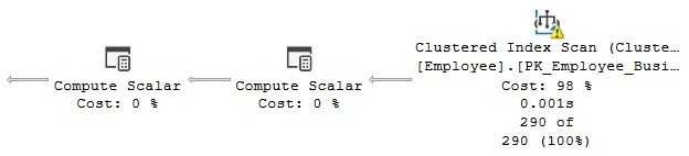
Figure 1.12 – Plan showing a ColumnsWithNoStatistics warning

Notice the warning (the symbol with an exclamation mark) on the Clustered Index Scan operator. If you look at its properties, you will see Columns With No Statistics: [AdventureWorks2019].[HumanResources].[Employee].VacationHours.

Note

Throughout this book, we may decide to show only part of the execution plan. Although you can see the entire plan on SQL Server Management Studio, our purpose is to improve the quality of the image by just showing the required operators.

Don’t forget to reenable the automatic creation of statistics by running the following command. There is no need to create the statistics object that was dropped previously because it can be created automatically if needed:

ALTER DATABASE AdventureWorks2019 SET AUTO_CREATE_STATISTICS ON

NoJoinPredicate

A possible problem while using the old-style ANSI SQL-89 join syntax is accidentally missing the join predicate and getting a NoJoinPredicate warning. Let’s suppose you intend to run the following query but forgot to include the WHERE clause:

SELECT * FROM Sales.SalesOrderHeader soh, Sales.SalesOrderDetail sod

WHERE soh.SalesOrderID = sod.SalesOrderID

The first indication of a problem could be that the query takes way too long to execute, even for small tables. Later, you will see that the query also returns a huge result set.

Sometimes, a way to troubleshoot a long-running query is to just stop its execution and request an estimated plan instead. If you don’t include the join predicate (in the WHERE clause), you will get the following plan:

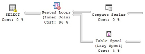
Figure 1.13 – Plan with a NoJoinPredicate warning

This time, you can see the warning on the Nested Loop Join as "No Join Predicate" with a different symbol. Notice that you cannot accidentally miss a join predicate if you use the ANSI SQL-92 join syntax because you get an error instead, which is why this syntax is recommended. For example, missing the join predicate in the following query will return an incorrect syntax error:

SELECT * FROM Sales.SalesOrderHeader soh JOIN Sales.SalesOrderDetail sod

-- ON soh.SalesOrderID = sod.SalesOrderID

Note

You can still get, if needed, a join whose result set includes one row for each possible pairing of rows from the two tables, also called a Cartesian product, by using the CROSS JOIN syntax.

PlanAffectingConvert

This warning shows that type conversions were performed that may impact the performance of the resulting execution plan. Run the following example, which declares the nvarchar variable and then uses it in a query to compare against a varchar column, CreditCardApprovalCode:

DECLARE @code nvarchar(15)

SET @code = '95555Vi4081'

SELECT * FROM Sales.SalesOrderHeader

WHERE CreditCardApprovalCode = @code

The query returns the following plan:

Figure 1.14 – Plan with a PlanAffectingConvert warning

The following two warnings are shown on the SELECT icon:

• The type conversion in the (CONVERT_IMPLICIT(nvarchar(15),[AdventureWorks2019].[Sales].[SalesOrderHeader].[CreditCardApprovalCode],0)) expression may affect CardinalityEstimate in the query plan choice.
• Type conversion in the (CONVERT_IMPLICIT(nvarchar(15),[AdventureWorks2019].[Sales].[SalesOrderHeader].[CreditCardApprovalCode],0)=[@code]) expression may affect SeekPlan in the query plan choice.

The recommendation is to use similar data types for comparison operations.

SpillToTempDb

This warning shows that an operation didn’t have enough memory and had to spill data to disk during execution, which can be a performance problem because of the extra I/O overhead. To simulate this problem, run the following example:

SELECT * FROM Sales.SalesOrderDetail

ORDER BY UnitPrice

This is a very simple query, and depending on the memory available on your system, you may not get the warning in your test environment, so you may need to try with a larger table instead. The plan shown in Figure 1.15 will be generated.

This time, the warning is shown on the Sort operator, which in my test included the message Operator used tempdb to spill data during execution with spill level 2 and 8 spilled thread(s), Sort wrote 2637 pages to and read 2637 pages from tempdb with granted memory 4096KB and used memory 4096KB. The XML plan also shows this:

<SpillToTempDb SpillLevel="2" SpilledThreadCount="8" />

<SortSpillDetails GrantedMemory="4096" UsedMemory="4096" WritesToTempDb="2637" ReadsFromTempDb="2637" />

This is shown here:

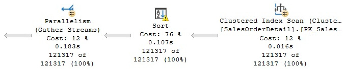
Figure 1.15 – Plan with a SpillToTempDb warning

UnmatchedIndexes

Finally, the UnmatchedIndexes element can show that the query optimizer was unable to match a filtered index for a particular query (for example, when it is unable to see the value of a parameter). Suppose you create the following filtered index:

CREATE INDEX IX_Color ON Production.Product(Name, ProductNumber)

WHERE Color = 'White'

Then, you run the following query:

DECLARE @color nvarchar(15)

SET @color = 'White'

SELECT Name, ProductNumber FROM Production.Product

WHERE Color = @color

The IX_Color index is not used at all, and you will get a warning on the plan, as shown here:

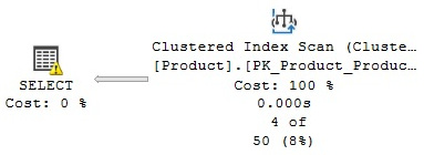
Figure 1.16 – Plan with an UnmatchedIndexes warning

Unfortunately, if you inspect the SELECT item in the graphical plan, it will not show any information about the warning at all. You will have to see the following on the XML plan (or by looking at the UnmatchedIndexes property of the SELECT operator’s properties window):

<UnmatchedIndexes>

<Parameterization>

<Object Database="[AdventureWorks2019]" Schema="[Production]"

Table="[Product]" Index="[IX_Color]" />

</Parameterization>

</UnmatchedIndexes>

<Warnings UnmatchedIndexes="true" />

However, the following query will use the index:

SELECT Name, ProductNumber FROM Production.Product

WHERE Color = 'White'

Filtered indexes and the UnmatchedIndexes element will be covered in detail in Chapter 5, Working with Indexes. For now, remove the index we just created:

DROP INDEX Production.Product.IX_Color

Note

Many exercises in this book will require you to make changes in the AdventureWorks databases. Although the database is reverted to its original state at the end of every exercise, you may also consider refreshing a copy of the database after several changes or tests, especially if you are not getting the expected results.

Getting plans from a trace or the plan cache

So far, we have been testing getting execution plans by directly using the query code in SQL Server Management Studio. However, this method may not always produce the plan you want to troubleshoot or the plan creating the performance problem. One of the reasons for this is that your application might be using a different SET statement option than SQL Server Management Studio and producing an entirely different execution plan for the same query. This behavior, where two plans may exist for the same query, will be covered in more detail in Chapter 8, Understanding Plan Caching.

Because of this behavior, sometimes, you may need to capture an execution plan from other locations, for example, the plan cache or current query execution. In these cases, you may need to obtain an execution plan from a trace, for example, using SQL trace or extended events, or the plan cache using the sys.dm_exec_query_plan dynamic management function (DMF) or perhaps using some collected data, as in the case of SQL Server Data Collector. Let’s take a look at some of these sources.

sys.dm_exec_query_plan DMF

As mentioned earlier, when a query is optimized, its execution plan may be kept in the plan cache. The sys.dm_exec_query_plan DMF can be used to return such cached plans, as well as any plan that is currently executing. However, when a plan is removed from the cache, it will no longer be available and the query_plan column of the returned table will be null.

For example, the following query shows the execution plans for all the queries currently running in the system. The sys.dm_exec_requests dynamic management view (DMV), which returns information about each request that’s currently executing, is used to obtain the plan_handle value, which is needed to find the execution plan using the sys.dm_exec_query_plan DMF. A plan_handle is a hash value that represents a specific execution plan, and it is guaranteed to be unique in the system:

SELECT * FROM sys.dm_exec_requests

CROSS APPLY sys.dm_exec_query_plan(plan_handle)

The output will be a result set containing the query_plan column, which shows links similar to the one shown in the XML plans section. As explained previously, clicking the link shows you requested the graphical execution plan.

In the same way, the following example shows the execution plans for all cached query plans. The sys.dm_exec_query_stats DMV contains one row per query statement within the cached plan and, again, provides the plan_handle value needed by the sys.dm_exec_query_plan DMF:

SELECT * FROM sys.dm_exec_query_stats

CROSS APPLY sys.dm_exec_query_plan(plan_handle)

Now, suppose you want to find the 10 most expensive queries by CPU usage. You can run the following query to get this information, which will return the average CPU time in microseconds per execution, along with the query execution plan:

SELECT TOP 10 

total_worker_time/execution_count AS avg_cpu_time, plan_handle, query_plan

FROM sys.dm_exec_query_stats

CROSS APPLY sys.dm_exec_query_plan(plan_handle)

ORDER BY avg_cpu_time DESC

SQL Trace/Profiler

You can also use SQL Trace and/or Profiler to capture the execution plans of queries that are currently executing. You can use the Performance event category in Profiler, which includes the following events:

• Performance Statistics
• Showplan All
• Showplan All For Query Compile
• Showplan Statistics Profile
• Showplan Text
• Showplan Text (Unencoded)
• Showplan XML
• Showplan XML For Query Compile
• Showplan XML Statistics Profile

To trace any of these events, run Profiler, connect to your SQL Server instance, click Events Selection, expand the Performance event category, and select any of the required events. You can select all the columns or only a subset of the columns, specify a column filter, and so on. Click Run to start the trace. The following screenshot shows an example of a trace with the Showplan XML event:

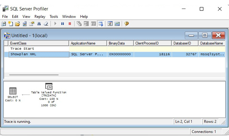
Figure 1.17 – A trace in Profiler showing the Showplan XML event

Optionally, you can create a server trace using a script, and even use Profiler as a scripting tool. To do that, define the events for your trace, run and stop the trace, and select File | Export | Script Trace Definition | For SQL Server 2005 – vNext…. This will produce the code to run a server trace, which will only be required to specify a filename to capture the trace. Part of the generated code is shown here:

/****************************************************/

/* Created by: SQL Server vNext CTP1.0 Profiler */

/* Date: 05/29/2022 08:37:22 AM */

/****************************************************/

-- Create a Queue

declare @rc int

declare @TraceID int

declare @maxfilesize bigint

set @maxfilesize = 5

-- Please replace the text InsertFileNameHere, with an appropriate

-- filename prefixed by a path, e.g., c:MyFolderMyTrace. The .trc extension

-- will be appended to the filename automatically. If you are writing from

-- remote server to local drive, please use UNC path and make sure server has

-- write access to your network share

exec @rc = sp_trace_create @TraceID output, 0, N'InsertFileNameHere', @maxfilesize,

NULL

if (@rc != 0) goto error

-- Client side File and Table cannot be scripted

-- Set the events

declare @on bit

set @on = 1

exec sp_trace_setevent @TraceID, 10, 1, @on

exec sp_trace_setevent @TraceID, 10, 9, @on

exec sp_trace_setevent @TraceID, 10, 2, @on

exec sp_trace_setevent @TraceID, 10, 66, @on

exec sp_trace_setevent @TraceID, 10, 10, @on

exec sp_trace_setevent @TraceID, 10, 3, @on

exec sp_trace_setevent @TraceID, 10, 4, @on

exec sp_trace_setevent @TraceID, 10, 6, @on

exec sp_trace_setevent @TraceID, 10, 7, @on

exec sp_trace_setevent @TraceID, 10, 8, @on

exec sp_trace_setevent @TraceID, 10, 11, @on

exec sp_trace_setevent @TraceID, 10, 12, @on

exec sp_trace_setevent @TraceID, 10, 13, @on

You may notice SQL Server vNext in a couple of places and even CTP1.0 being incorrectly shown. This was tested with SQL Server Profiler v19.0 Preview 2 and SQL Server 2022 CTP 2.0.

Note

As of SQL Server 2008, all non-XML events mentioned earlier, such as Showplan All, Showplan Text, and so on, are deprecated. Microsoft recommends using the XML events instead. SQL Trace has also been deprecated as of SQL Server 2012. Instead, Microsoft recommends using extended events.

For more details about using Profiler and SQL Trace, please refer to the SQL Server documentation.

Note

The SQL Server documentation used to be referred to as SQL Server Books Online, which was a component that could be optionally installed on your server. Recently, you are more likely to find such documentation on the web, such as at docs.microsoft.com/en-us/sql.

Extended events

You can also use extended events to capture execution plans. Although in general, Microsoft recommends using extended events over SQL Trace, as mentioned earlier, the events to capture execution plans are expensive to collect on the current releases of SQL Server. The documentation shows the following warning for all three extended events available to capture execution plans: Using this event can have a significant performance overhead so it should only be used when troubleshooting or monitoring specific problems for brief periods of time.

You can create and start an extended events session by using CREATE EVENT SESSION and ALTER EVENT SESSION. You can also use the new graphic user interface introduced in SQL Server 2012. Here are the events related to execution plans:

• query_post_compilation_showplan: Occurs after a SQL statement is compiled. This event returns an XML representation of the estimated query plan that is generated when the query is compiled.
• query_post_execution_showplan: Occurs after a SQL statement is executed. This event returns an XML representation of the actual query plan.
• query_pre_execution_showplan: Occurs after a SQL statement is compiled. This event returns an XML representation of the estimated query plan that is generated when the query is optimized.

For example, let’s suppose you want to start a session to trace the query_post_execution_showplan event. You could use the following code to create the extended event session:

CREATE EVENT SESSION [test] ON SERVER

ADD EVENT sqlserver.query_post_execution_showplan(

ACTION(sqlserver.plan_handle)

WHERE ([sqlserver].[database_name]=N'AdventureWorks2019'))

ADD TARGET package0.ring_buffer

WITH (STARTUP_STATE=OFF)

GO

More details about extended events will be covered in Chapter 2, Troubleshooting Queries. In the meantime, you can notice that the ADD EVENT argument shows the event name (in this case, query_post_execution_showplan), ACTION refers to global fields you want to capture in the event session (in this case, plan_handle), and WHERE is used to apply a filter to limit the data you want to capture. The [sqlserver].[database_name]=N'AdventureWorks2019' predicate indicates that we want to capture events for the AdventureWorks2019 database only. TARGET is the event consumer, and we can use it to collect the data for analysis. In this case, we are using the ring buffer target. Finally, STARTUP_STATE is one of the extended event options, and it is used to specify whether or not this event session is automatically started when SQL Server starts.

Once the event session has been created, you can start it using the ALTER EVENT SESSION statement, as shown in the following example:

ALTER EVENT SESSION [test]

ON SERVER

STATE=START

You can use the Watch Live Data feature, introduced with SQL Server 2012, to view the data that’s been captured by the event session. To do that, expand the Management folder in Object Explorer | Extended Events | Sessions, right-click the extended event session, and select Watch Live Data.

You can also run the following code to see this data:

SELECT

event_data.value('(event/@name)[1]', 'varchar(50)') AS event_name,

event_data.value('(event/action[@name="plan_handle"]/value)[1]',

'varchar(max)') as plan_handle,

event_data.query('event/data[@name="showplan_xml"]/value/*') as showplan_xml,

event_data.value('(event/action[@name="sql_text"]/value)[1]',

'varchar(max)') AS sql_text

FROM( SELECT evnt.query('.') AS event_data

FROM

( SELECT CAST(target_data AS xml) AS target_data

FROM sys.dm_xe_sessions AS s

JOIN sys.dm_xe_session_targets AS t

ON s.address = t.event_session_address

WHERE s.name = 'test'

AND t.target_name = 'ring_buffer'

) AS data

CROSS APPLY target_data.nodes('RingBufferTarget/event') AS xevent(evnt)

) AS xevent(event_data)

Once you’ve finished testing, you need to stop and delete the event session. Run the following statements:

ALTER EVENT SESSION [test]

ON SERVER

STATE=STOP

GO

DROP EVENT SESSION [test] ON SERVER

Finally, some other SQL Server tools can allow you to see plans, including the Data Collector. The Data Collector was introduced with SQL Server 2008 and will be covered in Chapter 2, Troubleshooting Queries.

Removing plans from the plan cache

You can use a few different commands to remove plans from the plan cache. These commands, which will be covered in more detail in Chapter 8, Understanding Plan Caching, can be useful during your testing and should not be executed in a production environment unless the requested effect is desired. The DBCC FREEPROCCACHE statement can be used to remove all the entries from the plan cache. It can also accept a plan handle or a SQL handle to remove only specific plans, or a Resource Governor pool name to remove all the cache entries associated with it. The DBCC FREESYSTEMCACHE statement can be used to remove all the elements from the plan cache or only the elements associated with a Resource Governor pool name. DBCC FLUSHPROCINDB can be used to remove all the cached plans for a particular database.

Finally, although not related to the plan cache, the DBCC DROPCLEANBUFFERS statement can be used to remove all the buffers from the buffer pool. You can use this statement in cases where you want to simulate a query starting with a cold cache, as we will do in the next section.

SET STATISTICS TIME and IO statements

We will close this chapter with two statements that can give you additional information about your queries and that you can use as an additional tuning technique. These can be a great complement to execution plans to get additional information about your queries’ optimization and execution. One common misunderstanding we sometimes see is developers trying to compare plan cost to plan performance. You should not assume a direct correlation between a query-estimated cost and its actual runtime performance. Cost is an internal unit used by the query optimizer and should not be used to compare plan performance; SET STATISTICS TIME and SET STATISTICS IO can be used instead. This section explains both statements.

You can use SET STATISTICS TIME to see the number of milliseconds required to parse, compile, and execute each statement. For example, run the following command:

SET STATISTICS TIME ON

Then, run the following query:

SELECT DISTINCT(CustomerID)

FROM Sales.SalesOrderHeader

To see the output, you will have to look at the Messages tab of the Edit window, which will show an output similar to the following:

SQL Server parse and compile time:

CPU time = 16 ms, elapsed time = 226 ms.

SQL Server Execution Times:

CPU time = 16 ms, elapsed time = 148 ms.

parse and compile time refers to the time SQL Server takes to optimize the SQL statement, as explained earlier. You can get similar information by looking at the QueryTimeStats query property, as shown earlier in this chapter. SET STATISTICS TIME will continue to be enabled for any subsequently executed queries. You can disable it like so:

SET STATISTICS TIME OFF

As mentioned previously, parse and compile information can also be seen on the execution plan, as shown here:

<QueryPlan DegreeOfParallelism="1" CachedPlanSize="16" CompileTime="226"

CompileCPU="9" CompileMemory="232">

If you only need the execution time of each query, you can see this information in Management Studio Query Editor.

SET STATISTICS IO displays the amount of disk activity generated by a query. To enable it, run the following statement:

SET STATISTICS IO ON

Run the following statement to clean all the buffers from the buffer pool to make sure that no pages for this table are loaded in memory:

DBCC DROPCLEANBUFFERS

Then, run the following query:

SELECT * FROM Sales.SalesOrderDetail

WHERE ProductID = 870

You will see an output similar to the following:

Table 'SalesOrderDetail'. Scan count 1, logical reads 1246, physical reads 3,

read-ahead reads 1277, lob logical reads 0, lob physical reads 0,

lob read-ahead reads 0.

Here are the definitions of these items, which all use 8K pages:

• Logical reads: Number of pages read from the buffer pool.
• Physical reads: Number of pages read from disk.
• Read-ahead reads: Read-ahead is a performance optimization mechanism that anticipates the needed data pages and reads them from disk. It can read up to 64 contiguous pages from one data file.
• Lob logical reads: Number of large object (LOB) pages read from the buffer pool.
• Lob physical reads: Number of LOB pages read from disk.
• Lob read-ahead reads: Number of LOB pages read from disk using the read-ahead mechanism, as explained earlier.

Now, if you run the same query again, you will no longer get physical and read-ahead reads. Instead, you will get an output similar to the following:

Table 'SalesOrderDetail'. Scan count 1, logical reads 1246, physical reads 0,

read-ahead reads 0, lob logical reads 0, lob physical reads 0,

lob read-ahead reads 0.

Scan count is defined as the number of seeks or scans started after reaching the leaf level (that is, the bottom level of an index). The only case when Scan count will return 0 is when you’re seeking only one value on a unique index, as shown in the following example:

SELECT * FROM Sales.SalesOrderHeader

WHERE SalesOrderID = 51119

If you try running the following query, in which SalesOrderID is defined in a non-unique index and can return more than one record, you will see that Scan count now returns 1:

SELECT * FROM Sales.SalesOrderDetail

WHERE SalesOrderID = 51119

Finally, in the following example, the scan count is 4 because SQL Server must perform four seeks:

SELECT * FROM Sales.SalesOrderHeader

WHERE SalesOrderID IN (51119, 43664, 63371, 75119)

Summary

In this chapter, we showed you how a better understanding of what the query processor does behind the scenes can help both database administrators and developers write better queries, as well as provide the query optimizer with the information it needs to produce efficient execution plans. In the same way, we showed you how to use your newfound knowledge of the query processor’s inner workings and SQL Server tools to troubleshoot cases when your queries are not performing as expected. Based on this, the basics of the query optimizer, the execution engine, and the plan cache were explained. These SQL Server components will be covered in greater detail later in this book.

Because we will be using execution plans throughout this book, we also introduced you to how to read them, their more important properties, and how to obtain them from sources such as the plan cache and a server trace. This should have given you enough background to follow along with the rest of this book. Query operators were also introduced but will be covered in a lot more detail in Chapter 4, The Execution Engine, and other sections of this book.

In the next chapter, we will explore additional tuning tools and techniques, such as using SQL Trace, extended events, and DMVs, to find out which queries are consuming the most resources or investigate some other performance-related problems.