Chapter 5: Working with Indexes
Indexing is one of the most important techniques used in query tuning and optimization. By using the right indexes, SQL Server can speed up your queries and drastically improve the performance of your applications. In this chapter, we will introduce indexes and show you how SQL Server uses them, how you can provide better indexes, and how you can verify that your execution plans are using these indexes correctly. There are several kinds of indexes in SQL Server. This chapter focuses on clustered and nonclustered indexes and discusses several topics, including covering indexes, filtered indexes, how to choose a clustered index key, and index fragmentation. Chapter 11, An Introduction to Data Warehouses, covers columnstore indexes in detail. Memory-optimized nonclustered indexes and hash indexes are covered in Chapter 7, In-Memory OLTP. Other types of indexes, such as XML, spatial, and full-text indexes, are outside the scope of this book.
This chapter also includes sections about the Database Engine Tuning Advisor (DTA) and the Missing Indexes feature, which will show you how you can use the query optimizer itself to provide index-tuning recommendations. However, it is important to emphasize that, no matter what index recommendations these tools give, it is ultimately up to the database administrator or developer to do their own index analysis, test these recommendations thoroughly, and finally decide which of these recommendations to implement.
Finally, the sys.dm_db_index_usage_stats DMV is introduced as a tool to identify existing indexes that are not being used by your queries. Indexes that are not being used will provide no benefit to your databases, use valuable disk space, and slow down your update operations, so they should be considered for removal.
This chapter covers the following topics:
- Introduction to indexes
- Creating indexes
- Understanding index operations
- The Database Engine Tuning Advisor
- Missing indexes
- Index fragmentation
- Unused indexes
Introduction to indexes
As mentioned in Chapter 4, The Execution Engine, SQL Server can use indexes to perform seek and scan operations. Indexes can be used to speed up the execution of a query by quickly finding records, without performing table scans, by delivering all of the columns requested by the query without accessing the base table (that is, covering the query, which we will return to later), or by providing a sorted order, which will benefit queries with GROUP BY, DISTINCT, or ORDER BY clauses.
Part of the query optimizer’s job is to determine whether an index can be used to resolve a predicate in a query. This is basically a comparison between an index key and a constant or variable. In addition, the query optimizer needs to determine whether the index covers the query—that is, whether the index contains all of the columns required by the query (in which case it is referred to as a covering index). The query optimizer needs to confirm this because a nonclustered index usually contains only a subset of the columns in the table.
SQL Server can also consider using more than one index and joining them to cover all of the columns required by the query. This operation is called “index intersection.” If it’s not possible to cover all of the columns required by the query, SQL Server may need to access the base table, which could be a clustered index or a heap, to obtain the remaining columns. This is called a bookmark lookup operation (which could be a key lookup or an RID lookup operation, as explained in Chapter 4, The Execution Engine). However, because a bookmark lookup requires random I/O, which is a very expensive operation, its usage can be effective only for a relatively small number of records.
Also, keep in mind that although one or more indexes could be used, that does not mean that they will finally be selected in an execution plan, as this is always a cost-based decision. So, after creating an index, make sure you verify that the index is in fact used in a plan and, of course, that your query is performing better, which is probably the primary reason why you are defining an index. An index that is not being used by any query will just take up valuable disk space and may negatively affect the performance of update operations without providing any benefit. It is also possible that an index that was useful when it was originally created is no longer used by any query now; this could be a result of changes in the database, the data, or even the query itself. To help you avoid this situation, the last section in this chapter shows you how you can identify which indexes are no longer being used by any of your queries. Let’s get started with creating indexes in the next section.
Creating indexes
Let’s start this section with a summary of some basic terminology used in indexes, some of which may already have been mentioned in previous chapters of the book, as follows:
- Heap: A heap is a data structure where rows are stored without a specified order. In other words, it is a table without a clustered index.
- Clustered index: In SQL Server, you can have the entire table logically sorted by a specific key in which the bottom, or leaf level, of the index contains the actual data rows of the table. Because of this, only one clustered index per table is possible. The data pages in the leaf level are linked in a doubly linked list (that is, each page has a pointer to the previous and next pages). Both clustered and nonclustered indexes are organized as B-trees.
- Nonclustered index: A nonclustered index row contains the index key values and a pointer to the data row on the base table. Nonclustered indexes can be created on both heaps and clustered indexes. Each table can have up to 999 nonclustered indexes, but usually, you should keep this number to a minimum. A nonclustered index can optionally contain non-key columns when using the INCLUDE clause, which is particularly useful when covering a query.
- Unique index: As the name suggests, a unique index does not allow two rows of data to have identical key values. A table can have one or more unique indexes, although it should not be very common. By default, unique indexes are created as nonclustered indexes unless you specify otherwise.
- Primary key: A primary key is a key that uniquely identifies each record in the table and creates a unique index, which, by default, will also be a clustered index. In addition to the uniqueness property required for the unique index, its key columns are required to be defined as NOT NULL. By definition, only one primary key can be defined on a table.
Although creating a primary key is straightforward, something not everyone is aware of is that when a primary key is created, by default, it is created using a clustered index. This can be the case, for example, when using Table Designer in SQL Server Management Studio (Table Designer is accessed when you right-click Tables and select New Table…) or when using the CREATE TABLE and ALTER TABLE statements, as shown next. If you run the following code to create a primary key, where the CLUSTERED or NONCLUSTERED keywords are not specified, the primary key will be created using a clustered index as follows:
CREATE TABLE table1 (
col1 int NOT NULL,
col2 nchar(10) NULL,
CONSTRAINT PK_table1 PRIMARY KEY(col1)
)
Or it can be created using the following code:
CREATE TABLE table1
(
col1 int NOT NULL,
col2 nchar(10) NULL
)
GO
ALTER TABLE table1 ADD CONSTRAINT
PK_table1 PRIMARY KEY
(
col1
)
The code generated by Table Designer will explicitly request a clustered index for the primary key, as in the following code (but this is usually hidden and not visible to you):
ALTER TABLE table1 ADD CONSTRAINT
PK_table1 PRIMARY KEY CLUSTERED
(
col1
)
Creating a clustered index along with a primary key can have some performance consequences, as we will see later on in this chapter, so it is important to understand that this is the default behavior. Obviously, it is also possible to have a primary key that is a nonclustered index, but this needs to be explicitly specified. Changing the preceding code to create a nonclustered index will look like the following code, where the CLUSTERED clause was changed to NONCLUSTERED:
ALTER TABLE table1 ADD CONSTRAINT
PK_table1 PRIMARY KEY NONCLUSTERED
(
col1
)
After the preceding code is executed, PK_table1 will be created as a unique nonclustered index.
Although the preceding code created an index as part of a constraint definition (in this case, a primary key), most likely, you will be using the CREATE INDEX statement to define indexes. The following is a simplified version of the CREATE INDEX statement:
CREATE [UNIQUE ] [ CLUSTERED | NONCLUSTERED ] INDEX index_name
ON <object> ( column [ ASC | DESC ] [ ,...n ] )
[ INCLUDE ( column_name [ ,...n ] ) ]
[ WHERE <filter_predicate> ]
[ WITH ( <relational_index_option> [ ,...n ] ) ]
The UNIQUE clause creates a unique index in which no two rows are permitted to have the same index key value. CLUSTERED and NONCLUSTERED define clustered and nonclustered indexes, respectively. The INCLUDE clause allows you to specify non-key columns to be added to the leaf level of the nonclustered index. The WHERE <filter_predicate> clause allows you to create a filtered index that will also create filtered statistics. Filtered indexes and the INCLUDE clause will be explained in more detail later on in this section. The WITH <relational_index_option> clause specifies the options to use when the index is created, such as FILLFACTOR, SORT_IN_TEMPDB, DROP_EXISTING, or ONLINE.
In addition, the ALTER INDEX statement can be used to modify an index and perform operations such as disabling, rebuilding, and reorganizing indexes. The DROP INDEX statement will remove the specified index from the database. Using DROP INDEX with a nonclustered index will remove the index data pages from the database. Dropping a clustered index will not delete the index data but keep it stored as a heap instead.
Let’s do a quick exercise to show some of the concepts and T-SQL statements mentioned in this section. Create a new table by running the following statement:
SELECT * INTO dbo.SalesOrderDetail
FROM Sales.SalesOrderDetail
Let’s use the sys.indexes catalog view to inspect the table properties as follows:
SELECT * FROM sys.indexes
WHERE object_id = OBJECT_ID('dbo.SalesOrderDetail')As shown in the following results (not all the columns are listed), a heap will be created as described in the type and type_desc columns. A heap always has an index_id value of 0:

Let’s create a nonclustered index as follows:
CREATE INDEX IX_ProductID ON dbo.SalesOrderDetail(ProductID)
The sys.indexes catalog now shows the following, where you can see that in addition to the heap, we now have a nonclustered index with index_id as 2. Nonclustered indexes can have index_id values between 2 and 250 and between 256 and 1,005. This range covers the maximum of 999 nonclustered indexes mentioned earlier. The values between 251 and 255 are reserved as follows:

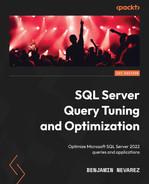
Now create a clustered index as follows:
CREATE CLUSTERED INDEX IX_SalesOrderID_SalesOrderDetailID
ON dbo.SalesOrderDetail(SalesOrderID, SalesOrderDetailID)
Note that instead of a heap, now we have a clustered index and the index_id value is now 1. A clustered index always has an index_id value of 1. Internally, the nonclustered index has been rebuilt to now use a cluster key pointer rather than a row identifier (RID).

Dropping the nonclustered index will remove the index pages entirely, leaving only the clustered index as follows:
DROP INDEX dbo.SalesOrderDetail.IX_ProductID
But notice that deleting the clustered index, which is considered the entire table, does not delete the underlying data; it simply changes the table structure to be a heap as follows:
DROP INDEX dbo.SalesOrderDetail.IX_SalesOrderID_SalesOrderDetailID

For more details about the CREATE INDEX, ALTER INDEX, and DROP INDEX statements, refer to the SQL Server documentation.
As shown in Figure 5.1, a clustered index is organized as a B-tree, which consists of a root node (the top node of the B-tree), leaf nodes (the bottom-level nodes, which contain the data pages of the table), and intermediate levels (the nodes between the root and leaf nodes). To find a specific record on a clustered index B-tree, SQL Server uses the root- and intermediate-level nodes to navigate to the leaf node, as the root and intermediate nodes contain index pages and a pointer to either an intermediate-level page or a leaf node page. To put this in perspective, and based on the example in Figure 5.1, with only one intermediate level, SQL Server is required to read three pages to find a specific row. A table with a larger number of records could have more than one intermediate level, requiring SQL Server to read four or more pages to find a row. This is the operation performed by an Index Seek operator, and it is very effective when only one row is required or when a partial scan can be used to satisfy the query.
However, this operation can be very expensive when it needs to be performed for many records, each one requiring access to at least three pages. This is the problem we usually face when we have a nonclustered index that does not cover the query and needs to look at the clustered index for the remaining columns required by the table. In this case, SQL Server has to navigate on both the B-tree of the nonclustered index and the clustered index. The query optimizer places a high cost on these operations, and this is why sometimes when a large number of records is required by the query, SQL Server decides to perform a clustered index scan instead. More details about these operations are provided in Chapter 4, The Execution Engine.

Figure 5.1 – Structure of a clustered index
Clustered indexes versus heaps
One of the main decisions you have to make when creating a table is whether to use a clustered index or a heap. Although the best solution may depend on your table definition and workload, it is usually recommended that each table be defined with a clustered index, and this section will show you why. Let’s start with a summary of the advantages and disadvantages of organizing tables as clustered indexes or heaps. Some of the good reasons to leave a table as a heap are the following:
- When the heap is a very small table. Although, a clustered index could work fine for a small table, too.
- When an RID is smaller than a candidate clustered index key. As introduced in Chapter 4, individual rows in a heap are identified by an RID, which is a row locator that includes information such as the database file, page, and slot numbers to allow a specific record to be easily located. An RID uses 8 bytes and, in many cases, could be smaller than a clustered index key. Because every row in every nonclustered index contains the RID or the clustered index key to point to the corresponding record on the base table, a smaller size could greatly benefit the number of resources used.
You definitely want to use a clustered index in the following cases:
- You frequently need to return data in a sorted order or query ranges of data. In this case, you would need to create the clustered index key in the column’s desired order. You may need the entire table in a sorted order or only a range of the data. Examples of the last operation, called a partial ordered scan, were provided in Chapter 4.
- You frequently need to return data grouped together. In this case, you would need to create the clustered index key on the columns used by the GROUP BY clause. As you learned in Chapter 4, to perform aggregate operations, SQL Server requires sorted data, and if it is not already sorted, a likely expensive sort operation may need to be added.
In the white paper SQL Server Best Practices Article, available at http://technet.microsoft.com/en-us/library/cc917672.aspx, the authors performed a series of tests to show the difference in performance while using heaps and clustered indexes. Although these tests may or may not resemble your own schema, workload, or application, you could use them as a guideline to estimate the impact on your application.
The test used a clustered index with three columns as the clustered index key and no other nonclustered index and compared it with a heap with only one nonclustered index defined using the same three columns. You can look at the paper for more details about the test, including the test scenarios. The interesting results shown by the six tests in the research are as follows:
- The performance of INSERT operations on a table with a clustered index was about 3 percent faster than performing the same operation on a heap with a corresponding nonclustered index. The reason for this difference is that even though inserting data into the heap had 62.8 percent fewer page splits/second, writing into the clustered index required a single write operation, whereas inserting the data on the heap required two—one for the heap and another for the nonclustered index.
- The performance of UPDATE operations on a nonindexed column in a clustered index was 8.2 percent better than performing the same operation on a heap with a corresponding nonclustered index. The reason for this difference is that updating a row on the clustered index only required an Index Seek operation, followed by an update of the data row; however, for the heap, it required an Index Seek operation using the nonclustered index, followed by an RID lookup to find the corresponding row on the heap, and finally an update of the data row.
- The performance of DELETE operations on a clustered index was 18.25 percent faster than performing the same operation on a heap with a corresponding nonclustered index. The reason for this difference is that, similar to the preceding UPDATE case, deleting a row on the clustered index only required an Index Seek operation, followed by a delete of the data row; however, for the heap, it required an Index Seek operation using the nonclustered index, followed by an RID lookup to find the corresponding row on the heap, and finally a delete. In addition, the row on the nonclustered index had to be deleted as well.
- The performance of a single-row SELECT operation on a clustered index was 13.8 percent faster than performing the same operation on a heap with a corresponding nonclustered index. This test assumes that the search predicate is based on the index keys. Again, finding a row in a clustered index only required a seek operation, and once the row was found, it contained all of the required columns. In the case of the heap, once again, it required an Index Seek operation using the nonclustered index, followed by an RID lookup to find the corresponding row on the heap.
- The performance of a SELECT operation on a range of rows on a clustered index was 29.41 percent faster than performing the same operation on a heap with a corresponding nonclustered index. The specific query selected 228 rows. Once again, a Clustered Index Seek operation helped to find the first record quickly, and, because the rows are stored in the order of the indexed columns, the remaining rows would be on the same pages or contiguous pages. As mentioned earlier, selecting a range of rows, called a partial ordered scan, is one of the cases where using a clustered index is definitely a superior choice to using a heap, because fewer pages must be read. Also, keep in mind that in this scenario, the cost of performing multiple lookups may be so high in some cases that the query optimizer may decide to scan the entire heap instead. That is not the case for the clustered index, even if the specified range is large.
- For the disk utilization test following INSERT operations, the test showed little difference between the clustered index and a heap with a corresponding nonclustered index. However, for the disk utilization test following DELETE operations, the clustered index test showed a significant difference between the clustered index and a heap with a corresponding nonclustered index. The clustered index shrunk almost the same amount as the amount of data deleted, whereas the heap shrunk only a fraction of it. The reason for this difference is that empty extents are automatically deallocated in a clustered index, which is not the case for heaps where the extents are held onto for later reuse. Recovering this unused disk space on a heap usually requires additional tasks, such as performing a table rebuild operation (using the ALTER TABLE REBUILD statement).
- For the concurrent INSERT operations, the test showed that as the number of processes that are concurrently inserting data increases, the amount of time per insert also increases. This increase is more significant in the case of the clustered index compared with the heap. One of the main reasons for this was the contention found while inserting data in a particular location. The test showed that the page latch waits per second were 12 percent higher for the clustered index compared with the heap when 20 processes were concurrently inserting data, and this value grew to 61 percent when 50 concurrent processes inserted data. However, the test found that for the case of the 50 concurrent sessions, the overhead per insert was only an average of 1.2 milliseconds per insert operation and was not considered significant.
- Finally, because the heap required a nonclustered index to provide the same seek benefits as the clustered index, the disk space used by the clustered index was almost 35 percent smaller than the table organized as a heap.
The research paper concluded that, in general, the performance benefits of using a clustered index outweigh the negatives according to the tests performed. Finally, it is worth remembering that although clustered indexes are generally recommended, your performance may vary depending on your own table schema, workload, and specific configuration, so you may want to test both choices carefully.
Clustered index key
Deciding which column or columns will be part of the clustered index key is also a very important design consideration because they need to be chosen carefully. As a best practice, indexes should be unique, narrow, static, and ever-increasing. But remember that, as with other general recommendations, this may not apply to all cases, so you should also test thoroughly for your database and workload. Let’s explain why these may be important and how they may affect the performance of your database as follows:
- Unique: If a clustered index is not defined using the UNIQUE clause, SQL Server will add a 4-byte uniquifier to each record, increasing the size of the clustered index key. As a comparison, an RID used by nonclustered indexes on heaps is only 8 bytes long.
- Narrow: As mentioned earlier in this chapter, because every row in every nonclustered index contains, in addition to the columns defining the index, the clustered index key to point to the corresponding row on the base table, a small-sized key could greatly benefit the number of resources used. A small key size will require less storage and memory, which will also benefit performance. Again, as a comparison, an RID used by nonclustered indexes on heaps is only 8 bytes long.
- Static or nonvolatile: Updating a clustered index key can have some performance consequences, such as page splits and fragmentation created by the row relocation within the clustered index. In addition, because every nonclustered index contains the clustered index key, the changing rows in the nonclustered index will have to be updated as well to reflect the new clustered key value.
- Ever-increasing: A clustered index key would benefit from having ever-increasing values instead of having more random values, such as in the last name column, for example. Having to insert new rows based on random entry points creates page splits and therefore fragmentation. However, you need to be aware that, in some cases, having ever-increasing values can also cause contention, as multiple processes could be written on the last page of a table.
Covering indexes
A covering index is a very simple but very important concept in query optimization where an index can solve or is able to return all of the columns requested by a query without accessing the base table at all. For example, the following query is already covered by an existing index, IX_SalesOrderHeader_CustomerID, as you can see in the plan in Figure 5.2:
SELECT SalesOrderID, CustomerID FROM Sales.SalesOrderHeader
WHERE CustomerID = 16448
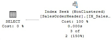
Figure 5.2 – A covering index
In the plan, we can see that there is no need to access the base table at all. If we slightly change the query to also request the SalesPersonID column, this time there is no index that covers the query, and the plan in Figure 5.3 is produced instead, as follows:
SELECT SalesOrderID, CustomerID, SalesPersonID FROM Sales.SalesOrderHeader
WHERE CustomerID = 16448
Figure 5.3 – A plan with a key lookup operation
The plan shows that IX_SalesOrderHeader_CustomerID was used to quickly locate the required record, but because the index didn’t include SalesPersonID, a lookup operation to the clustered index was required as well. Keep in mind that trying to cover the query does not mean that you need to add another column to the index key unless you must also perform search operations using that column. Instead, you could use the INCLUDE clause of the CREATE or ALTER INDEX statements to add the additional column. At this point, you may decide to just update an existing index to include the required column, but in the following example, we will create another one:
CREATE INDEX IX_SalesOrderHeader_CustomerID_SalesPersonID
ON Sales.SalesOrderHeader(CustomerID)
INCLUDE (SalesPersonID)
If you run the query again, the query optimizer will use a plan similar to the one shown previously in Figure 5.2 with just an Index Seek operation, this time with the new IX_SalesOrderHeader_CustomerID_SalesPersonID index and no need to access the base table at all. However, notice that creating many indexes on a table can also be a performance problem because multiple indexes need to be updated on each update operation, not to mention the additional disk space required.
Finally, to clean up, drop the temporarily created index as follows:
DROP INDEX Sales.SalesOrderHeader.IX_SalesOrderHeader_CustomerID_SalesPersonID
Filtered indexes
You can use filtered indexes in queries where a column only has a small number of relevant values. This can be the case, for example, when you want to focus your query on some specific values in a table where a column has mostly NULL values and you need to query the non-NULL values. Handily, filtered indexes can also enforce uniqueness within the filtered data. Filtered indexes have the benefit of requiring less storage than regular indexes, and maintenance operations on them will be faster as well. In addition, a filtered index will also create filtered statistics, which may have a better quality than a statistics object created for the entire table, as a histogram will be created just for the specified range of values. As covered in more detail in Chapter 6, Understanding Statistics, a histogram can have up to a maximum of 200 steps, which can be a limitation with a large number of distinct values. To create a filtered index, you need to specify a filter using the WHERE clause of the CREATE INDEX statement.
For example, if you look at the plan for the following query, you will see that it uses both IX_SalesOrderHeader_CustomerID to filter on the CustomerID = 13917 predicate plus a key lookup operation to find the records on the clustered index and filter for TerritoryID = 4 (remember from Chapter 4 that in this case, a key lookup is really a Clustered Index Seek operator, which you can directly see if you use the SET SHOWPLAN_TEXT statement):
SELECT CustomerID, OrderDate, AccountNumber FROM Sales.SalesOrderHeader
WHERE CustomerID = 13917 AND TerritoryID = 4
Create the following filtered index:
CREATE INDEX IX_CustomerID ON Sales.SalesOrderHeader(CustomerID)
WHERE TerritoryID = 4
If you run the previous SELECT statement again, you will see a similar plan as shown in Figure 5.4, but in this case, using the just-created filtered index. Index Seek is doing a seek operation on CustomerID, but the key lookup no longer has to filter on TerritoryID because IX_CustomerID already filtered that out:
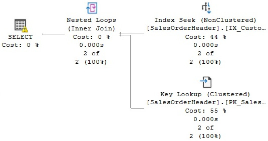
Figure 5.4 – Plan using a filtered index
Keep in mind that although the filtered index may not seem to provide more query performance benefits than a regular nonclustered index defined with the same properties, it will use less storage, will be easier to maintain, and can potentially provide better optimizer statistics because the filtered statistics will be more accurate since they cover only the rows in the filtered index.
However, a filtered index may not be used to solve a query when a value is not known, for example, when using variables or parameters. Because the query optimizer has to create a plan that can work for every possible value in a variable or parameter, the filtered index may not be selected. As introduced in Chapter 1, An Introduction to Query Tuning and Optimization, you may see the UnmatchedIndexes warning in an execution plan in these cases. Using our current example, the following query will show an UnmatchedIndexes warning, indicating that the plan was not able to use the IX_CustomerID index, even when the value requested for TerritoryID was 4, the same used in the filtered index:
DECLARE @territory int
SET @territory = 4
SELECT CustomerID, OrderDate, AccountNumber FROM Sales.SalesOrderHeader
WHERE CustomerID = 13917 AND TerritoryID = @territory
Drop the index before continuing, as follows:
DROP INDEX Sales.SalesOrderHeader.IX_CustomerID
Now that we have learned how to create and use indexes, we will explore some basic operations that can be performed on them.
Understanding index operations
In a seek operation, SQL Server navigates throughout the B-tree index to quickly find the required records without the need for an index or table scan. This is similar to using an index at the end of a book to find a topic quickly, instead of reading the entire book. Once the first record has been found, SQL Server can then scan the index leaf level forward or backward to find additional records. Both equality and inequality operators can be used in a predicate, including =, <, >, <=, >=, <>, !=, !<, !>, BETWEEN, and IN. For example, the following predicates can be matched to an Index Seek operation if there is an index on the specified column or a multicolumn index with that column as a leading index key:
- ProductID = 771
- UnitPrice < 3.975
- LastName = ‘Allen’
- LastName LIKE ‘Brown%’
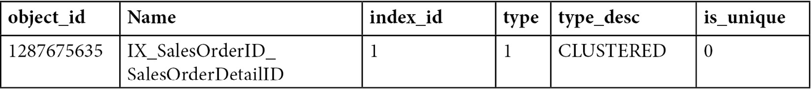
As an example, look at the following query, which uses an Index Seek operator and produces the plan in Figure 5.5:
SELECT ProductID, SalesOrderID, SalesOrderDetailID
FROM Sales.SalesOrderDetail
WHERE ProductID = 771

Figure 5.5 – Plan using an Index Seek
The SalesOrderDetail table has a multicolumn index with ProductID as the leading column. The Index Seek operator properties, which you can inspect in a graphical plan, include the following Seek predicate on the ProductID column, which shows that SQL Server was effectively able to use the index to seek on this column:
Seek Keys[1]: Prefix: [AdventureWorks2019].[Sales]. [SalesOrderDetail].ProductID = Scalar Operator (CONVERT_IMPLICIT(int,[@1],0))
An index cannot be used to seek on some complex expressions, expressions using functions, or strings with a leading wildcard character, as in the following predicates:
- ABS(ProductID) = 771
- UnitPrice + 1 < 3.975
- LastName LIKE '%Allen'
- UPPER(LastName) = 'Allen'
Compare the following query to the preceding example; by adding an ABS function to the predicate, SQL Server is no longer able to use an Index Seek operator and instead chooses to do an Index Scan, as shown in the plan in Figure 5.6:
SELECT ProductID, SalesOrderID, SalesOrderDetailID
FROM Sales.SalesOrderDetail
WHERE ABS(ProductID) = 771

Figure 5.6 – Plan using an Index Scan
If you look at the properties of the Index Scan operator, for example, in a graphical plan, you could verify that the following predicate is used:
abs([AdventureWorks2019].[Sales].[SalesOrderDetail].[ProductID])=CONVERT_IMPLICIT(int,[@1],0)
In the case of a multicolumn index, SQL Server can only use the index to seek on the second column if there is an equality predicate on the first column. So, SQL Server can use a multicolumn index to seek on both columns in the following cases, supposing that a multicolumn index exists on both columns in the order presented:
- ProductID = 771 AND SalesOrderID > 34000
- LastName = 'Smith' AND FirstName = 'Ian'
That being said, if there is no equality predicate on the first column, or if the predicate cannot be evaluated on the second column, as is the case in a complex expression, then SQL Server may still only be able to use a multicolumn index to seek on just the first column, as in the following examples:
- ProductID < 771 AND SalesOrderID = 34000
- LastName > 'Smith' AND FirstName = 'Ian'
- ProductID = 771 AND ABS(SalesOrderID) = 34000
However, SQL Server is not able to use a multicolumn index for an Index Seek in the following examples because it is not even able to search on the first column:
- ABS(ProductID) = 771 AND SalesOrderID = 34000
- LastName LIKE ‘%Smith’ AND FirstName = 'Ian'
Finally, run the following query and take a look at the Index Seek operator properties:
SELECT ProductID, SalesOrderID, SalesOrderDetailID
FROM Sales.SalesOrderDetail
WHERE ProductID = 771 AND ABS(SalesOrderID) = 45233
The Seek predicate is using only the ProductID column as follows:
Seek Keys[1]: Prefix: [AdventureWorks2019].[Sales].[SalesOrderDetail].ProductID =
Scalar Operator (CONVERT_IMPLICIT(int,[@1],0)
An additional predicate on the SalesOrderID column is evaluated like any other scan predicate as follows:
abs([AdventureWorks2019].[Sales].[SalesOrderDetail]. [SalesOrderID])=[@2]
In summary, this shows that, as we expected, SQL Server was able to perform a seek operation on the ProductID column, but, because of the use of the ABS function, it was not able to do the same for SalesOrderID. The index was used to navigate directly to find the rows that satisfy the first predicate but then had to continue scanning to validate the second predicate.
The Database Engine Tuning Advisor
Currently, all major commercial database vendors include a physical database design tool to help with the creation of indexes. However, when these tools were first developed, there were just two main architectural approaches considered for how the tools should recommend indexes. The first approach was to build a stand-alone tool with its own cost model and design rules. The second approach was to build a tool that could use the query optimizer cost model.
A problem with building a stand-alone tool is the requirement for duplicating the cost module. On top of that, having a tool with its own cost model, even if it’s better than the query optimizer’s cost model, may not be a good idea because the optimizer still chooses its plan based on its own model.
The second approach, using the query optimizer to help with physical database design, was proposed in the database research community as far back as 1988. Because it is the query optimizer that chooses the indexes for an execution plan, it makes sense to use the query optimizer itself to help find which missing indexes would benefit existing queries. In this scenario, the physical design tool would use the optimizer to evaluate the cost of queries given a set of candidate indexes. An additional benefit of this approach is that, as the optimizer cost model evolves, any tool using its cost model can automatically benefit from it.
SQL Server was the first commercial database product to include a physical design tool, in the shape of the Index Tuning Wizard, which was shipped with SQL Server 7.0 and was later replaced by the DTA in SQL Server 2005. Both tools use the query optimizer cost model approach and were created as part of the AutoAdmin project at Microsoft, the goal of which was to reduce the total cost of ownership (TCO) of databases by making them self-tuning and self-managing. In addition to indexes, the DTA can help with the creation of indexed views and table partitioning.
However, creating real indexes in a DTA tuning session is not feasible; its overhead could affect operational queries and degrade the performance of your database. So how does the DTA estimate the cost of using an index that does not yet exist? Actually, even during regular query optimization, the query optimizer does not use indexes to estimate the cost of a query. The decision on whether to use an index or not relies only on some metadata and statistical information regarding the columns of the index. Index data itself is not needed during query optimization, but will, of course, be required during query execution if the index is chosen.
So, to avoid creating real indexes during a DTA session, SQL Server uses a special kind of index called hypothetical indexes, which were also used by the Index Tuning Wizard. As the name implies, hypothetical indexes are not real indexes; they only contain statistics and can be created with the undocumented WITH STATISTICS_ONLY option of the CREATE INDEX statement. You may not be able to see these indexes during a DTA session because they are dropped automatically when they are no longer needed. However, you could see the CREATE INDEX WITH STATISTICS_ONLY and DROP INDEX statements if you run a SQL Server Profiler session to see what the DTA is doing.
Let’s take a quick tour of some of these concepts. To get started, create a new table on the AdventureWorks2019 database as follows:
SELECT * INTO dbo.SalesOrderDetail
FROM Sales.SalesOrderDetail
Then copy the following query and save it to a file:
SELECT * FROM dbo.SalesOrderDetail
WHERE ProductID = 897
Open a new DTA session. The DTA is found in the Tools menu in SQL Server Management Studio with the full name Database Engine Tuning Advisor. You can optionally run a SQL Server Profiler session if you want to inspect what the DTA is doing. On the Workload File option, select the file containing the SQL statement that you just created and then specify AdventureWorks2019 as both the database to tune and the database for workload analysis. Click the Start Analysis button and, when the DTA analysis finishes, run the following query to inspect the contents of the msdb..DTA_reports_query table:
SELECT * FROM msdb..DTA_reports_query
Running the preceding query shows the following output (edited for space):

Notice that the query returns information such as the query that was tuned as well as the current and recommended cost. The current cost, 1.2471, is easy to obtain by directly requesting an estimated execution plan for the query, as shown in Figure 5.7:
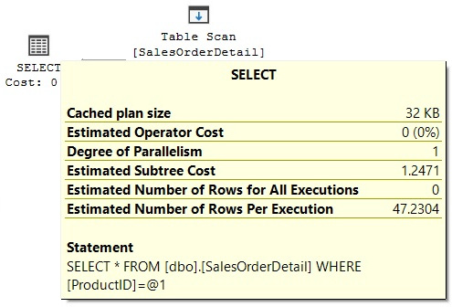
Figure 5.7 – Plan showing the total cost
Since the DTA analysis was completed, the required hypothetical indexes were already dropped. To obtain the indexes recommended by the DTA, click the Recommendations tab and look at the Index Recommendations section, where you can find the code to create any recommended index by clicking the Definition column. In our example, it will show the following code:
CREATE CLUSTERED INDEX [_dta_index_SalesOrderDetail_c_5_1440724185__K5]
ON [dbo].[SalesOrderDetail]
(
[ProductID] ASC
)WITH (SORT_IN_TEMPDB = OFF, DROP_EXISTING = OFF, ONLINE = OFF) ON [PRIMARY]
In the following statement, and for demonstration purposes only, we will go ahead and create the index recommended by the DTA. However, instead of a regular index, we will create it as a hypothetical index by adding the WITH STATISTICS_ONLY clause. Keep in mind that hypothetical indexes cannot be used by your queries and are only useful for the DTA:
CREATE CLUSTERED INDEX cix_ProductID ON dbo.SalesOrderDetail(ProductID)
WITH STATISTICS_ONLY
You can validate that a hypothetical index was created by running the following query:
SELECT * FROM sys.indexes
WHERE object_id = OBJECT_ID('dbo.SalesOrderDetail')AND name = 'cix_ProductID'
The output is as follows (note that the is_hypothetical field shows that this is, in fact, just a hypothetical index):

Remove the hypothetical index by running the following statement:
DROP INDEX dbo.SalesOrderDetail.cix_ProductID
Finally, implement the DTA recommendation, creating the _dta_index_SalesOrderDetail_c_5_1440724185__K5 index, as previously indicated. After implementing the recommendation and running the query again, the clustered index is, in fact, now being used by the query optimizer. This time, the plan shows a Clustered Index Seek operator and an estimated cost of 0.0033652, which is very close to the recommended cost listed when querying the msdb..DTA_reports_query table.
Tuning a workload using the plan cache
In addition to the traditional options for tuning a workload using the File or Table choices, which allow you to specify a script or a table containing the T-SQL statements to tune, starting with SQL Server 2012, you can also specify the plan cache as a workload to tune. In this case, the DTA will select the top 1,000 events from the plan cache based on the total elapsed time of the query (that is, based on the total_elapsed_time column of the sys.dm_exec_query_stats DMV, as explained in Chapter 2). Let’s try an example, and to make it easy to see the results, let’s clear the plan cache and run only one query in SQL Server Management Studio as follows:
DBCC FREEPROCCACHE
GO
SELECT SalesOrderID, OrderQty, ProductID
FROM dbo.SalesOrderDetail
WHERE CarrierTrackingNumber = 'D609-4F2A-9B'
After the query is executed, most likely, it will be kept in the plan cache. Open a new DTA session. In the Workload option, select Plan Cache and specify AdventureWorks2019 as both the database to tune and the database for workload analysis. Click the Start Analysis button. After the analysis is completed, you can select the Recommendations tab and select Index Recommendations, which will include the following recommendations (which you can see by looking at the Definition column):
CREATE NONCLUSTERED INDEX [_dta_index_SalesOrderDetail_5_807673925__K3_1_4_5]
ON [dbo].[SalesOrderDetail]
(
[CarrierTrackingNumber] ASC
)
INCLUDE ([SalesOrderID],
[OrderQty],
[ProductID]) WITH (SORT_IN_TEMPDB = OFF, DROP_EXISTING = OFF, ONLINE = OFF)
ON [PRIMARY]
Finally, drop the table you just created by running the following statement:
DROP TABLE dbo.SalesOrderDetail
Offload of tuning overhead to test server
One of the most interesting and perhaps lesser-known features of the DTA is that you can use it with a test server to tune the workload of a production server. As mentioned earlier, the DTA relies on the query optimizer to make its tuning recommendations, and you can use it to make these optimizer calls to a test server instance without affecting the performance of the production server.
To better understand how this works, let’s first review what kind of information the query optimizer needs to optimize a query. Basically, the most important information it needs to perform an optimization is the following:
- The database metadata (that is, table and column definitions, indexes, constraints, and so on)
- Optimizer statistics (index and column statistics)
- Table size (number of rows and pages)
- Available memory and number of processors
The DTA can gather the database metadata and statistics from the production server and use them to create a similar database, with no data, on a different server. This database is called a shell database. The DTA can also obtain the available memory and number of processors on the production server by using the xp_msver extended stored procedure and use this information for the optimization process. It is important to remember that no data is needed for the optimization process. This process is summarized in Figure 5.8:
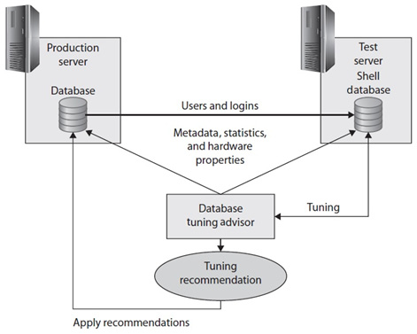
Figure 5.8 – Using a test server and a shell database with the DTA
This process provides the following benefits:
- There is no need to do an expensive optimization on the production server, which can affect its resource usage. The production server is only used to gather initial metadata and the required statistics.
- There is no need to copy the entire database to a test server either (which is especially important for big databases), thus saving disk space and time to copy the database.
- There are no problems where test servers are not as powerful as production servers because the DTA tuning session will consider the available memory and number of processors on the production server.
Let’s now see an example of how to run a tuning session. First of all, the use of a test server is not supported by the DTA graphical user interface, so the use of the dta utility (the command-prompt version of DTA) is required. Configuring a test server also requires an XML input file containing the dta input information. We will be using the following input file (saved as input.xml) for this example. You will need to change production_instance and test_instance where appropriate. These must also be different SQL Server instances, as follows:
<?xml version=”1.0” encoding=”utf-16” ?>
<DTAXML xmlns:xsi=”http://www.w3.org/2001/XMLSchema-instance”
xmlns=”http://schemas.microsoft.com/sqlserver/2004/07/dta”>
<DTAInput>
<Server>
<Name>production_instance</Name>
<Database>
<Name>AdventureWorks2019</Name>
</Database>
</Server>
<Workload>
<File>workload.sql</File>
</Workload>
<TuningOptions>
<TestServer>test_instance</TestServer>
<FeatureSet>IDX</FeatureSet>
<Partitioning>NONE</Partitioning>
<KeepExisting>NONE</KeepExisting>
</TuningOptions>
</DTAInput>
</DTAXML>
The Server and Database elements of the XML file include the production SQL Server instance and database. The Workload element includes the definition of a script containing the workload to tune. TuningOptions includes the TestServer sub-element, which is used to include the name of the test SQL Server instance.
Create the workload.sql file containing a simple query as follows:
SELECT * FROM AdventureWorks2019.Sales.SalesOrderDetail
WHERE ProductID = 898
Run the following command (note the difference in –S and –s because case is important here):
dta -ix input.xml -S production_instance -s session1
If the dta utility is not reachable with your current PATH environment variable, you can find it either on your SQL Server or your SQL Server Management Studio installation. For example, older versions of SQL Server may have it at C:Program FilesMicrosoft SQL Server nnToolsBinn, assuming you installed the software on the C: volume. Our current installation points to C:Program Files (x86)Microsoft SQL Server Management Studio 19Common7.
A successful execution will show the following output:
Microsoft (R) SQL Server Microsoft SQL Server Database Engine Tuning Advisor command line utility
Version 16.0.19056.0 ((SSMS_Rel_19).220520-2253)
Copyright (c) Microsoft. All rights reserved.
Tuning session successfully created. Session ID is 3.
Total time used: 00:00:49
Workload consumed: 100%, Estimated improvement: 88%
Tuning process finished.
This example creates an entire copy of AdventureWorks2019 (with no data) and performs the requested optimization. The shell database is automatically deleted after the tuning session is completed. Optionally, you can keep the shell database (for example, if you want to use it again on another tuning exercise) by using RetainShellDB in the TuningOptions element, as in the following XML fragment:
<TuningOptions>
<TestServer>test_instance</TestServer>
<FeatureSet>IDX</FeatureSet>
<Partitioning>NONE</Partitioning>
<KeepExisting>NONE</KeepExisting>
<RetainShellDB>1</RetainShellDB>
</TuningOptions>
If the shell database already exists when you request a tuning session, the database creation process will be skipped. However, you will have to manually delete this database when it is no longer needed.
Once the tuning session is completed, you can use the DTA graphical user interface as usual to see the recommendations. To do this, open the DTA, open the session you used by double-clicking its session name (session1 in our example), and choose the Recommendations tab if it is not already selected.
Although the DTA automatically gathers the metadata and statistics to build the shell database, we will see how to script the required objects and statistics to tune a simple query. This can be helpful in cases where you don’t want to script the entire database. Scripting database objects is a fairly simple process well known by SQL Server professionals. Something that may be new for many, though, is how to script the statistics. Created scripts make use of the undocumented STATS_STREAM, ROWCOUNT, and PAGECOUNT options of the CREATE/UPDATE STATISTICS statement.
As an example, to optimize the simple query shown earlier, try the following steps in SQL Server Management Studio:
- Expand Databases in Object Explorer.
- Right-click the AdventureWorks2019 database, select Tasks | Generate Scripts, and then click Next.
- Select Select specific database objects.
- Expand Tables.
- Select Sales.SalesOrderDetail and click Next.
- Click Advanced.
- Look for the Script Statistics choice and select Script statistics and histograms.
- Choose True on Script Indexes.
Your Advanced Scripting Options window should look similar to Figure 5.9:

Figure 5.9 – Advanced Scripting Options window
Click OK to finish the wizard and generate the scripts. You will get a script with a few UPDATE STATISTICS statements similar to the following (with the STAT_STREAM value shortened to fit on this page):
UPDATE STATISTICS [Sales].[SalesOrderDetail]([IX_SalesOrderDetail_ProductID])
WITH STATS_STREAM = 0x0100000003000000000000000000000041858B2900000000141A00 …,
ROWCOUNT = 121317, PAGECOUNT = 274
These UPDATE STATISTICS statements are used to update the statistics of existing indexes (obviously, the related CREATE INDEX statements were scripted as well). If the table also has column statistics, it will include CREATE STATISTICS statements instead.
Finally, we will see an example of how to use scripted statistics to obtain plans and cost estimates on an empty table. Running the following query on the regular AdventureWorks2019 database creates the following plan with an estimated number of rows of 9 and a cost of 0.0296836:
SELECT * FROM Sales.SalesOrderDetail
WHERE ProductID = 898
Let’s produce the same plan on a new and empty database. First, create the Sales schema as follows:
CREATE SCHEMA Sales
Following the procedure described earlier, you can script the Sales.SalesOrderDetail table. You will end up with multiple statements, including the following statements (again shortened to fit in this space). Although the script created many statements, the following are the minimum statements required for this exercise:
CREATE TABLE [Sales].[SalesOrderDetail](
[SalesOrderID] [int] NOT NULL,
…
) ON [PRIMARY]
GO
CREATE NONCLUSTERED INDEX [IX_SalesOrderDetail_ProductID] ON [Sales].[SalesOrderDetail]
(
[ProductID] ASC
)
GO
UPDATE STATISTICS [Sales].[SalesOrderDetail]([IX_SalesOrderDetail_ProductID])
WITH STATS_STREAM = 0x0100000003000000000000000000000041858B2900000000141A00 …,
ROWCOUNT = 121317, PAGECOUNT = 274
GO
UPDATE STATISTICS [Sales].[SalesOrderDetail]([PK_SalesOrderDetail_SalesOrderID_SalesOrderDetailID])
WITH STATS_STREAM = 0x0100000002000000000000000000000051752A6300000000431500 …,
ROWCOUNT = 121317, PAGECOUNT = 1237
Run at least the preceding four statements using the scripts you got in the previous step (note that this text does not include the entire statement—it is only shown for reference). After implementing the script on an empty database and running the sample query, you will again get the plan with a cost of 0.0296836 and an estimated number of rows of 9.
Missing indexes
SQL Server provides a second approach that can help you find useful indexes for your existing queries. Although not as powerful as the DTA, this option, called the missing indexes feature, does not require the database administrator to decide when tuning is needed, to explicitly identify what workload represents the load to tune, or to run any tool. This is a lightweight feature that is always on and, like the DTA, was also introduced with SQL Server 2005. Let’s take a look at what it does.
During optimization, the query optimizer defines what the best indexes for a query are and, if these indexes don’t exist, it will make this index information available in the query XML plan (which is also available in a graphical plan in SQL Server Management Studio 2008 or later). Alternatively, it will aggregate this information for optimized queries since the instance was started, and make it all available on the sys.dm_db_missing_index DMVs. Note that just by displaying this information, the query optimizer is not only warning you that it might not be selecting an efficient plan, but it is also showing you which indexes may help to improve the performance of your query. In addition, database administrators and developers should be aware of the limitations of this feature, as described in “Limitations of the Missing Indexes Feature,” at http://msdn.microsoft.com/en-us/library/ms345485(v=sql.105).aspx.
So, with all that in mind, let’s take a quick look to see how this feature works. Create the dbo.SalesOrderDetail table on the AdventureWorks2019 database by running the following statement:
SELECT * INTO dbo.SalesOrderDetail
FROM Sales.SalesOrderDetail
Run the following query and request a graphical or XML execution plan:
SELECT * FROM dbo.SalesOrderDetail
WHERE SalesOrderID = 43670 AND SalesOrderDetailID > 112
This query could benefit from an index on the SalesOrderID and SalesOrderDetailID columns, but no missing indexes information is shown this time. One limitation of the missing indexes feature that this example has revealed is that it does not work with a trivial plan optimization. You can verify that this is a trivial plan by looking at the graphical plan properties, shown as Optimization Level TRIVIAL, or by looking at the XML plan, where StatementOptmLevel is shown as TRIVIAL. You can avoid trivial plan optimization in several ways, as explained in Chapter 3, The Query Optimizer. In our case, we’re just going to create a non-related index by running the following statement:
CREATE INDEX IX_ProductID ON dbo.SalesOrderDetail(ProductID)
What is significant about this is that, although the index created will not be used by our previous query, the query no longer qualifies for a trivial plan. Run the query again, and this time the XML plan will contain the following entry:
<MissingIndexes>
<MissingIndexGroup Impact=”99.7142”>
<MissingIndex Database=”[AdventureWorks2019]” Schema=”[dbo]”
Table=”[SalesOrderDetail]”>
<ColumnGroup Usage=”EQUALITY”>
<Column Name=”[SalesOrderID]” ColumnId=”1” />
</ColumnGroup>
<ColumnGroup Usage=”INEQUALITY”>
<Column Name=”[SalesOrderDetailID]” ColumnId=”2” />
</ColumnGroup>
</MissingIndex>
</MissingIndexGroup>
</MissingIndexes>
The MissingIndexes entry in the XML plan can show up to three groups—equality, inequality, and included—and the first two are shown in this example using the ColumnGroup attribute. The information contained in these groups can be used to create the missing index; the key of the index can be built by using the equality columns, followed by the inequality columns, and the included columns can be added using the INCLUDE clause of the CREATE INDEX statement. Management Studio (versions SQL Server 2008 and later) can build the CREATE INDEX statement for you. In fact, if you look at the graphical plan, you can see a Missing Index warning at the top, including a CREATE INDEX command, as shown in Figure 5.10:

Figure 5.10 – Plan with a Missing Index warning
Notice the impact value of 99.7142. Impact is a number between 0 and 100 that gives you an estimate of the average percentage benefit that the query could obtain if the proposed index were available. You can right-click the graphical plan and select Missing Index Details to see the CREATE INDEX command that can be used to create this desired index as follows:
/*
Missing Index Details from SQLQuery1.sql - (local).AdventureWorks2019
The Query Processor estimates that implementing the following index could
improve the query cost by 99.7142%.
*/
/*
USE [AdventureWorks2019]
GO
CREATE NONCLUSTERED INDEX [<Name of Missing Index, sysname,>]
ON [dbo].[SalesOrderDetail] ([SalesOrderID],[SalesOrderDetailID])
GO
*/
Create the recommended index, after you provide a name for it, by running the following statement:
CREATE NONCLUSTERED INDEX IX_SalesOrderID_SalesOrderDetailID
ON [dbo].[SalesOrderDetail]([SalesOrderID], [SalesOrderDetailID])
If you run our previous SELECT statement again and look at the execution plan, this time you’ll see an Index Seek operator using the index you’ve just created, and both the Missing Index warning and the MissingIndex element of the XML plan are gone.
Finally, remove the dbo.SalesOrderDetail table you’ve just created by running the following statement:
DROP TABLE dbo.SalesOrderDetail
So far, we have discussed how to use indexes to optimize query performance. Let’s end the chapter with a couple of sections about the maintenance of indexes.
Index fragmentation
Although SQL Server automatically maintains indexes after any INSERT, UPDATE, DELETE, or MERGE operation, some index maintenance activities on your databases may still be required, mostly due to index fragmentation. Fragmentation happens when the logical order of pages in an index does not match the physical order in the data file. Because fragmentation can affect the performance of some queries, you need to monitor the fragmentation level of your indexes and, if required, perform reorganize or rebuild operations on them.
It is also worth clarifying that fragmentation may affect only queries performing scans or range scans; queries performing Index Seeks may not be affected at all. The query optimizer does not consider fragmentation either, so the plans it produces will be the same whether you have high fragmentation or no fragmentation at all. The query optimizer does not consider whether the pages in an index are in a physical order or not. However, one of the inputs for the query optimizer is the number of pages used by a table or index, and this number of pages may increase when there is a lot of unused space.
You can use the sys.dm_db_index_physical_stats DMF to analyze the fragmentation level of your indexes; you can query this information for a specific partition or index, or look at all of the indexes on a table, database, or even the entire SQL Server instance. The following example will return fragmentation information for the Sales.SalesOrderDetail of the AdventureWorks2019 database:
SELECT a.index_id, name, avg_fragmentation_in_percent, fragment_count,
avg_fragment_size_in_pages
FROM sys.dm_db_index_physical_stats (DB_ID('AdventureWorks2019'),OBJECT_ID('Sales.SalesOrderDetail'), NULL, NULL, NULL) AS aJOIN sys.indexes AS b ON a.object_id = b.object_id AND a.index_id = b.index_id
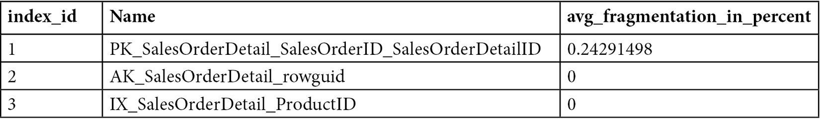
In our copy of AdventureWorks2019, we got the following output (not all the columns are shown to fit the page):

Although the level of fragmentation considered a problem may vary and depend on your database and application, a best practice is to reorganize indexes with more than 10 percent and up to 30 percent fragmentation. An index rebuild operation could be more appropriate if you have fragmentation greater than 30 percent. A fragmentation of 10 percent or less should not be considered a problem.
An index reorganization operation defragments the leaf level of clustered and nonclustered indexes and is always an online operation. When rebuilding an index, you can optionally use the ONLINE = ON clause to perform an online operation for most of the index rebuild operation (a very short phase at the beginning and the end of the operation will not allow concurrent user activity). Rebuilding an index drops and re-creates the index and removes fragmentation by compacting the index pages based on the specified or existing fill factor configuration. The fill factor is a value from 1 to 100 that specifies a percentage that indicates how full the leaf level of each index page must be during index creation or alteration.
To rebuild all of the indexes on the SalesOrderDetail table, use the following statement:
ALTER INDEX ALL ON Sales.SalesOrderDetail REBUILD
Here is the fragmentation in our copy of AdventureWorks2019 after running the preceding statement:
If you need to reorganize the index, which is not the case here, you can use a command such as the following:
ALTER INDEX ALL ON Sales.SalesOrderDetail REORGANIZE
As mentioned earlier, fragmentation can also be removed from a heap by using the ALTER TABLE REBUILD statement. However, this could be an expensive operation because it causes all nonclustered indexes to be rebuilt as the heap RIDs obviously change. Rebuilding an index also has an impact on statistics maintenance. For more details about index and statistics maintenance, see Chapter 6, Understanding Statistics.
Unused indexes
We will end this chapter on indexes by introducing the functionality of the sys.dm_db_index_usage_stats DMV, which you can use to learn about the operations performed by your indexes. It is especially helpful in discovering indexes that are not used by any query or are only minimally used. As we’ve already discussed, indexes that are not being used will provide no benefit to your databases but will use valuable disk space and slow your update operations, so they should be considered for removal.
The sys.dm_db_index_usage_stats DMV stores the number of seek, scan, lookup, and update operations performed by both user and system queries, including the last time each type of operation was performed, and its counters are reset when the SQL Server service starts. Keep in mind that this DMV, in addition to nonclustered indexes, will also include heaps, listed as index_id equal to 0, and clustered indexes, listed as index_id equal to 1. For this section, you may want to just focus on nonclustered indexes, which include index_id values of 2 or greater. Because heaps and clustered indexes contain the table’s data, they may not even be candidates for removal in the first place.
By inspecting the user_seeks, user_scans, and user_lookup values of your nonclustered indexes, you can see how your indexes are being used, and you can also look at the user_updates values to see the number of updates performed on the index. All of this information will help give you a sense of how useful an index actually is. Bear in mind that all we will be demonstrating is how to look up information from this DMV and what sort of situations will trigger different updates to the information it returns.
As an example, run the following code to create a new table with a nonclustered index:
SELECT * INTO dbo.SalesOrderDetail
FROM Sales.SalesOrderDetail
CREATE NONCLUSTERED INDEX IX_ProductID ON dbo.SalesOrderDetail(ProductID)
If you want to keep track of the values for this example, follow these steps carefully, because every query execution may change the index usage statistics. When you run the following query, it will initially contain only one record, which was created because of table access performed when the IX_ProductID index was created:
SELECT DB_NAME(database_id) AS database_name,
OBJECT_NAME(s.object_id) AS object_name, i.name, s.*
FROM sys.dm_db_index_usage_stats s JOIN sys.indexes i
ON s.object_id = i.object_id AND s.index_id = i.index_id
AND OBJECT_ID('dbo.SalesOrderDetail') = s.object_idHowever, the values that we will be inspecting in this exercise—user_seeks, user_scans, user_lookups, and user_updates—are all set to 0. Now run the following query, let’s say, three times:
SELECT * FROM dbo.SalesOrderDetail
This query is using a Table Scan operator, so, if you rerun our preceding query using the sys.dm_db_index_usage_stats DMV, it will show the value 3 on the user_scans column. Note that the index_id column is 0, denoting a heap, and the name of the table is also listed (as a heap is just a table with no clustered index). Run the following query, which uses an Index Seek, twice:
SELECT ProductID FROM dbo.SalesOrderDetail
WHERE ProductID = 773
After the query is executed, a new record will be added for the nonclustered index, and the user_seeks counter will show a value of 2.
Now, run the following query four times, and it will use both Index Seek and RID lookup operators:
SELECT * FROM dbo.SalesOrderDetail
WHERE ProductID = 773
Because user_seeks for the nonclustered index had a value of 2, it will be updated to 6, and the user_lookups value for the heap will be updated to 4.
Finally, run the following query once:
UPDATE dbo.SalesOrderDetail
SET ProductID = 666
WHERE ProductID = 927
Note that the UPDATE statement is doing an Index Seek and a Table Update, so user_seek will be updated for the index, and user_updates will be updated once for both the nonclustered index and the heap. The following is the final output of our query using the sys.dm_db_index_usage_stats DMV (edited for space):

Finally, drop the table you just created as follows:
DROP TABLE dbo.SalesOrderDetail
Summary
In this chapter, we introduced indexing as one of the most important techniques used in query tuning and optimization and covered clustered and nonclustered indexes. In addition, we discussed related topics such as how SQL Server uses indexes, how to choose a clustered index key, and how to fix index fragmentation.
We also explained how you can define the key of your indexes so that they are likely to be considered for seek operations, which can improve the performance of your queries by finding records more quickly. Predicates were analyzed in the contexts of both single and multicolumn indexes, and we also covered how to verify an execution plan to validate that indexes were selected and properly used by SQL Server.
The Database Engine Tuning Advisor and the missing indexes feature, both introduced with SQL Server 2005, were presented to show you how the query optimizer itself can indirectly be used to provide index-tuning recommendations.
Finally, we introduced the sys.dm_db_index_usage_stats DMV and its ability to provide valuable information regarding your nonclustered indexes usage. Although we didn’t discuss all the practicalities of using this DMV, we covered enough for you to be able to easily find nonclustered indexes that are not being used by your SQL Server instance.