Chapter 4: The Execution Engine

At its heart, the execution engine is a collection of physical operators that are software components performing the functions of the query processor. Their purpose is to execute your query efficiently. If we look at it from another perspective, the operations implemented by the execution engine define the choices available to the query optimizer when building execution plans. The execution engine and its operators were briefly covered in previous chapters. Now, we’ll cover some of the most used operators, their algorithms, and their costs in greater detail. In this chapter, we will focus on operators related to data access, joins, aggregations, parallelism, and updates, as these are the ones most commonly used in queries, and also the ones that are used more in this book. Of course, many more operators are implemented by the execution engine, and you can find a complete list and description within the official SQL Server 2022 documentation. This chapter illustrates how the query optimizer decides between the various choices of operators provided by the execution engine. For example, we will see how the query processor chooses between a Nested Loops Join operator and a Hash Join operator and between a Stream Aggregate operator and a Hash Aggregate operator.

In this chapter, we will look at the data access operations, including the operators to perform scans, seeks, and bookmark lookups on database structures, such as heaps, clustered indexes, and nonclustered indexes. The concepts of sorting and hashing are also explained, along with how they impact some of the algorithms of both physical joins and aggregations, which are detailed later. In the same way, the section on joins presents the Nested Loops Join, Merge Join, and Hash Join physical operators. The next section focuses on aggregations and explains the Stream Aggregate and Hash Aggregate operators in detail. The chapter continues with parallelism and explains how it can help to reduce the response time of a query. Finally, the chapter concludes by explaining how the query processor handles update operations.

This chapter covers the following topics:

• Data access operators
• Aggregations
• Joins
• Parallelism
• Updates

Data access operators

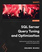
In this section, we will learn about the operations that directly access the database, using either a base table or an index, examples of which include scans and seeks. A scan reads an entire structure, which could be a heap, a clustered index, or a nonclustered index. On the other hand, a seek does not scan an entire structure, but instead efficiently retrieves rows by navigating an index. Therefore, seeks can only be performed on a clustered index or a nonclustered index. Just to make the difference between these structures clear, a heap contains all the table columns, and its data is not stored and sorted in any particular order. Conversely, in a clustered index, the data is stored logically, sorted by the clustering key, and in addition to the clustering key, the clustered index also contains the remaining columns of the table. On the other hand, a nonclustered index can be created on a clustered index or a heap and, usually, contains only a subset of the columns of the table. The operations of these structures are summarized in Table 4.1:

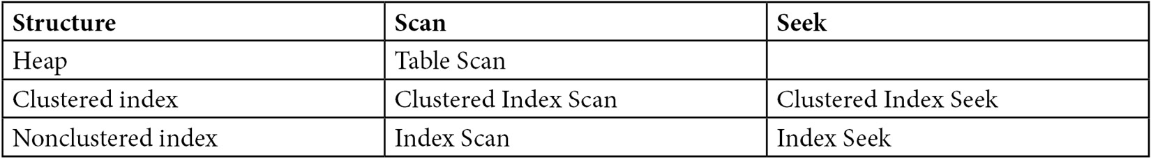
Table 4.1 – Data access operators

Scans

Let’s start with the simplest example—by scanning a heap, which is performed by the Table Scan operator, as shown in Table 4.1. The following query on the AdventureWorks2019 database will use a Table Scan operator, as shown in Figure 4.1:

SELECT * FROM DatabaseLog

Figure 4.1 – A Table Scan operator

Similarly, the following query will show a Clustered Index Scan operator, as shown in the plan of Figure 4.2. The Table Scan and Clustered Index Scan operations are similar in that they both scan the entire base table, but the former is used for heaps and the latter for clustered indexes:

SELECT * FROM Person.Address

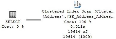
Figure 4.2 – A Clustered Index Scan operator

Many SQL Server users assume that because a Clustered Index Scan operator was used, the data returned will be automatically sorted. The reality is that even when the data in a clustered index has been stored and sorted, using a Clustered Index Scan operator does not guarantee that the results will be sorted unless it has been explicitly requested.

By not automatically sorting the results, the storage engine has the option to find the most efficient way to access this data without worrying about returning it in an ordered set. Examples of these efficient methods used by the storage engine include using an allocation order scan based on Index Allocation Map (IAM) pages and using an index order scan based on the index-linked list. In addition, an advanced scanning mechanism called merry-go-round scanning (which is an Enterprise Edition-only feature) allows multiple query executions to share full table scans so that each execution might join the scan at a different location, thus saving the overhead of each query having to separately read the data.

If you want to know whether your data has been sorted, the Ordered property can show you if the data was returned in a manner ordered by the Clustered Index Scan operator. So, for example, the clustering key of the Person.Address table is AddressID, and if you run the following query and look at the tooltip of the Clustered Index Scan operator in a graphical plan, you could validate that the Ordered property is true:

SELECT * FROM Person.Address

ORDER BY AddressID

This is also shown in the following XML fragment plan:

<IndexScan Ordered="true" ScanDirection="FORWARD" ForcedIndex="false" ForceSeek="false" … >

If you run the same query without the ORDER BY clause, the Ordered property will, unsurprisingly, show false. In some cases, SQL Server can benefit from reading the table in the order specified by the clustered index. Another example is shown in Figure 4.13, where a Stream Aggregate operator can benefit from the fact that a Clustered Index Scan operator can easily obtain the data that has already been sorted.

Next, we will see an example of an Index Scan operator. This example uses a nonclustered index to cover a query; that is, it can solve the entire query without accessing the base table (bearing in mind that a nonclustered index usually contains only a few of the columns of the table). Run the following query, which will show a plan that is similar to Figure 4.3:

SELECT AddressID, City, StateProvinceID

FROM Person.Address

Figure 4.3 – An Index Scan operator

Note that the query optimizer was able to solve this query without even accessing the Person.Address base table, and instead decided to scan the IX_Address_AddressLine1_AddressLine2_City_StateProvinceID_PostalCode index, which comprises fewer pages when compared to the clustered index. The index definition includes AddressLine1, AddressLine2, City, StateProvinceID, and PostalCode, so it can clearly cover columns requested in the query. However, you might be wondering where the index is getting the AddressID column from. When a nonclustered index is created on a table with a clustered index, each nonclustered index row also includes the table clustering key. This clustering key is used to find which record from the clustered index is referred to by the nonclustered index row (a similar approach for nonclustered indexes on a heap will be explained later). In this case, as I mentioned earlier, AddressID is the clustering key of the table, and it is stored in every row of the nonclustered index, which is why the index was able to cover this column in the previous query.

Seeks

Now, let’s look at Index Seeks. These can be performed by both Clustered Index Seek operators and Index Seek operators, which are used against clustered and nonclustered indexes, respectively. An Index Seek operator does not scan the entire index but instead navigates the B-tree index structure to quickly find one or more records. The next query, together with the plan in Figure 4.4, shows an example of a Clustered Index Seek operator. One benefit of a Clustered Index Seek operator, compared to a nonclustered Index Seek operator, is that the former can cover any column of the table. Of course, because the records of a clustered index are logically ordered by its clustering key, a table can only have one clustered index. If a clustered index was not defined, the table will, therefore, be a heap:

SELECT AddressID, City, StateProvinceID FROM Person.Address

WHERE AddressID = 12037

Figure 4.4 – A Clustered Index Seek operator

The next query and Figure 4.5 both illustrate a nonclustered Index Seek operator. Here, it is interesting to note that the base table was not used at all, and it was not even necessary to scan the entire index: there is a nonclustered index on the StateProvinceID parameter, and as mentioned previously, it also contains the clustering key, AddressID:

SELECT AddressID, StateProvinceID FROM Person.Address

WHERE StateProvinceID = 32

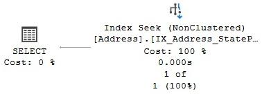
Figure 4.5 – An Index Seek operator

Although both examples that are shown only return one row, an Index Seek operation can also be used to find multiple rows with either equality or nonequality operators, which is called a partially ordered scan. The previous query just returned one row, but you can change it to a new parameter, such as in the following example:

SELECT AddressID, StateProvinceID FROM Person.Address

WHERE StateProvinceID = 9

The query has been auto-parameterized, and the same plan will be used with any other parameter. You can try to force a new optimization and plan (for example, using OPTION (RECOMPILE)), but the same plan will be returned. In this case, the same plan that was shown in Figure 4.5 will be used, and 4,564 rows will be returned without the need to access the base table at all. A partially ordered scan works by using the index to find the first row that qualifies and continues reading the remaining rows, which are all logically together on the same leaf pages of the index. More details about the index structure will be covered in Chapter 5, Working with Indexes. Parameterization is covered in greater detail in Chapter 8, Understanding Plan Caching.

A more complicated example of partially ordered scans involves using a nonequality operator or a BETWEEN clause, such as in the following example:

SELECT AddressID, City, StateProvinceID FROM Person.Address

WHERE AddressID BETWEEN 10000 and 20000

Because the clustered index is defined using AddressID, a plan similar to Figure 4.4 will be used, where a Clustered Index Seek operation will be used to find the first row that qualifies for the filter predicate and will continue scanning the index—row by row—until the last row that qualifies is found. More accurately, the scan will stop on the first row that does not qualify.

Bookmark lookup

Now, the question that comes up is what happens if a nonclustered index is useful for quickly finding one or more records, but does not cover the query? In other words, what happens if the nonclustered index does not contain all the columns requested by the query? In this case, the query optimizer has to decide whether it is more efficient to use the nonclustered index to find these records quickly and then access the base table to obtain the additional fields. Alternatively, it can decide whether it is more optimal to just go straight to the base table and scan it, reading each row and testing to see whether it matches the predicates. For example, in our previous query, an existing nonclustered index covers both the AddressID and StateProvinceID columns. What if we also request the City and ModifiedDate columns in the same query? This is shown in the next query, which returns one record and produces the same plan as Figure 4.6:

SELECT AddressID, City, StateProvinceID, ModifiedDate

FROM Person.Address

WHERE StateProvinceID = 32

Figure 4.6 – A bookmark lookup example

As you can see in the previous example, the query optimizer is choosing the IX_Address_StateProvinceID index to find the records quickly. However, because the index does not cover the additional columns, it also needs to use the base table (in this case, the clustered index) to get that additional information. This operation is called a bookmark lookup, and it is performed by the Key Lookup operator, which was introduced specifically to differentiate a bookmark lookup from a regular Clustered Index Seek operator. The Key Lookup operator only appears on a graphical plan (and then only from SQL Server 2005 Service Pack 2 and onward). Text and XML plans can show whether a Clustered Index Seek operator is performing a bookmark lookup by looking at the LOOKUP keyword and lookup attributes, as shown next. For example, let’s run the following query:

SET SHOWPLAN_TEXT ON

GO

SELECT AddressID, City, StateProvinceID, ModifiedDate

FROM Person.Address

WHERE StateProvinceID = 32

GO

SET SHOWPLAN_TEXT OFF

GO

The output will show the following text plan, including a Clustered Index Seek operator with the LOOKUP keyword at the end:

|--Nested Loops(Inner Join, OUTER REFERENCES …)

|--Index Seek(OBJECT:([Address].[IX_Address_StateProvinceID]),

SEEK:([Address].[StateProvinceID]=(32)) ORDERED FORWARD)

|--Clustered Index Seek(OBJECT:([Address].[PK_Address_AddressID]),

SEEK:([Address].[AddressID]=[Address].[AddressID]) LOOKUP ORDERED FORWARD)

The XML plan shows the same information in the following way:

<RelOp LogicalOp="Clustered Index Seek" PhysicalOp="Clustered Index Seek" …>

…

<IndexScan Lookup="true" Ordered="true" ScanDirection="FORWARD" …>

Bear in mind that although SQL Server 2000 implemented a bookmark lookup using a dedicated operator (called Bookmark Lookup), essentially, the operation is the same.

Now run the same query, but this time, request StateProvinceID equal to 20. This will produce the plan that is shown in Figure 4.7:

SELECT AddressID, City, StateProvinceID, ModifiedDate

FROM Person.Address

WHERE StateProvinceID = 20

Figure 4.7 – A plan switching to a Clustered Index Scan operator

In the preceding execution, the query optimizer has selected a Clustered Index Scan operator and the query has returned 308 records, compared to just a single record for the StateProvinceID value: 32. So, the query optimizer is producing two different execution plans for the same query, with the only difference being the value of the StateProvinceID parameter. In this case, the query optimizer uses the value of the query’s StateProvinceID parameter to estimate the cardinality of the predicate as it tries to produce an efficient plan for that parameter. We will learn more about this behavior, called parameter sniffing, in Chapter 8, Understanding Plan Caching, and Chapter 9, The Query Store. Additionally, we will learn how the estimation is performed in Chapter 6, Understanding Statistics.

This time, the query optimizer estimated that more records could be returned than when StateProvinceID was equal to 32, and it decided that it was cheaper to do a Table Scan than to perform many bookmark lookups. At this stage, you might be wondering what the tipping point is, in other words, at what point the query optimizer decides to change from one method to another. Because a bookmark lookup requires random I/Os, which is very expensive, it would not take many records for the query optimizer to switch from a bookmark lookup to a Clustered Index Scan (or a Table Scan) operator. We already know that when the query returned one record, for StateProvinceID 32, the query optimizer chose a bookmark lookup. Additionally, we saw that when we requested the records for StateProvinceID 20, which returned 308 records, it used a Clustered Index Scan operator. Logically, we can try requesting somewhere between 1 and 308 records to find this switchover point, right?

As you might already suspect, this is a cost-based decision that does not depend on the actual number of records returned by the query—rather, it is influenced by the estimated number of records. We can find these estimates by analyzing the histogram of the statistics object for the IX_Address_StateProvinceID index—something that will be covered in Chapter 6, Understanding Statistics.

We performed this exercise and found that the highest estimated number of records to get a bookmark lookup for this particular example was 62, and the first one to have a Clustered Index Scan operator was 106. Let’s look at both examples here by running the query with the StateProvinceID values of 163 and 71. We will get the plans that are shown in Figure 4.8 and Figure 4.9, respectively:

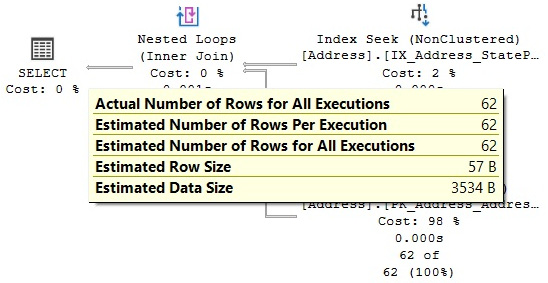
Figure 4.8 – The plan for the StateProvinceID = 163 predicate

The second plan is as follows:

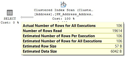
Figure 4.9 – The plan for the StateProvinceID = 71 predicate

Looking at the preceding plans, we can see that, for this specific example, the query optimizer selects a bookmark lookup for an estimated 62 records and changes to a Clustered Index Scan operator when that estimated number of records goes up to 106 (there are no estimated values between 62 and 106 for the histogram of this particular statistics object). Bear in mind that, although here, both the actual and estimated number of rows are the same, the query optimizer makes its decision based on the estimated number of rows. The actual number of rows is only known after the execution plan has been generated and executed, and the results are returned.

Finally, because nonclustered indexes can exist on both heaps and clustered indexes, we can also have a bookmark lookup on a heap. To follow the next example, create an index in the DatabaseLog table, which is a heap, by running the following statement:

CREATE INDEX IX_Object ON DatabaseLog(Object)

Then, run the following query, which will produce the plan shown in Figure 4.10:

SELECT * FROM DatabaseLog

WHERE Object = 'City'

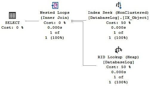
Figure 4.10 – A RID Lookup operator

Note that instead of the Key Lookup operator shown earlier, this plan displays a RID Lookup operator. This is because heaps do not have clustering keys in the same way that clustered indexes do, and instead, they use row identifiers (RIDs). A RID is a row locator that includes information such as the database file, page, and slot numbers to allow a specific record to be easily located. Every row in a nonclustered index created on a heap contains the RID of the corresponding heap record.

To clean up and leave tables in their original state, remove the index you just created:

DROP INDEX DatabaseLog.IX_Object

In this section, we have seen how the execution engine accesses our tables and indexes. In the following sections, we will see the most common operations performed on such data.

Aggregations

Aggregations are operations used in databases to summarize information about some set of data. The result of aggregate operations can be a single value, such as the average salary for a company, or it can be a per-group value, such as the average salary by department. SQL Server has two operators to implement aggregations, Stream Aggregate and Hash Aggregate, and they can be used to solve queries with aggregation functions (such as SUM, AVG, and MAX), or when using the GROUP BY clause and the DISTINCT keyword.

Sorting and hashing

Before introducing the remaining operators of this chapter, let’s discuss sorting and hashing, both of which play a very important role in some of the operators and algorithms of the execution engine. For example, two of the operators covered in this chapter, Stream Aggregate and Merge Join, require data to be already sorted. To provide sorted data, the query optimizer might employ an existing index, or it might explicitly introduce a Sort operator. On the other hand, hashing is used by the Hash Aggregate and Hash Join operators, both of which work by building a hash table in memory. The Hash Join operator only uses memory for the smaller of its two inputs, which is selected by the query optimizer.

Additionally, sorting uses memory and, similar to hashing operations, will also use the tempdb database if there is not enough available memory, which could become a performance problem. Both sorting and hashing are blocking operations (otherwise known as stop-and-go) meaning that they cannot produce any rows until they have consumed all of their input. In reality, this is only true for hashing operations during the time the build input is hashed, as explained later.

Stream Aggregate

Let’s start with the Stream Aggregate operator by using a query with an aggregation function. Queries using an aggregate function (and no GROUP BY clause) are called scalar aggregates, as they return a single value and are always implemented by the Stream Aggregate operator. To demonstrate this, run the following query, which shows the plan from Figure 4.11:

SELECT AVG(ListPrice) FROM Production.Product

Figure 4.11 – A Stream Aggregate operator

A text plan can be useful to show more details about both the Stream Aggregate and Compute Scalar operators. Run the following query:

SET SHOWPLAN_TEXT ON

GO

SELECT AVG(ListPrice) FROM Production.Product

GO

SET SHOWPLAN_TEXT OFF

Here is the displayed text plan:

|--Compute Scalar(DEFINE:([Expr1002]=CASE WHEN [Expr1003]=(0) THEN NULL ELSE

[Expr1004]/CONVERT_IMPLICIT(money,[Expr1003],0) END))

|--Stream Aggregate(DEFINE:([Expr1003]=Count(*), [Expr1004]=SUM([Product].

[ListPrice])))

|--Clustered Index Scan(OBJECT:([Product].[PK_Product_ProductID]))

The same information could be obtained from the graphical plan by selecting the Properties window (by pressing the F4 key) of both the Stream Aggregate and Compute Scalar operators and then opening the Defined Values property.

In any case, note that to implement the AVG aggregation function, the Stream Aggregate operator is computing both a COUNT aggregate and a SUM aggregate, the results of which will be stored in the computed expressions of Expr1003 and Expr1004, respectively. The Compute Scalar operator verifies that there is no division by zero when using a CASE expression. As you can see in the text plan if Expr1003 (which is the value for the count) is zero, the Compute Scalar operator returns NULL; otherwise, it calculates and returns the average by dividing the sum by the count.

Now, let’s see an example of a query—this time, using the GROUP BY clause. The following query produces the plan shown in Figure 4.12:

SELECT ProductLine, COUNT(*) FROM Production.Product

GROUP BY ProductLine

Figure 4.12 – Stream Aggregate using a Sort operator

A Stream Aggregate operator always requires its input to be sorted by the GROUP BY clause predicate. So, in this case, the Sort operator shown in the plan will provide the data sorted by the ProductLine column. After the sorted input has been received, the records for the same group will be next to each other, so the Stream Aggregate operator can now easily count the records for each group.

Note that although the first example in this section, using the AVG function, also used a Stream Aggregate operator, it did not require any sorted input. A query without a GROUP BY clause considers its entire input a single group.

A Stream Aggregate operator can also use an index to have its input sorted, as demonstrated in the following query, which produces the plan shown in Figure 4.13:

SELECT SalesOrderID, SUM(LineTotal)FROM Sales.SalesOrderDetail

GROUP BY SalesOrderID

Figure 4.13 – Stream Aggregate using an existing index

No Sort operator is needed in this plan because the Clustered Index Scan operator provides the data already sorted by SalesOrderID, which is part of the clustering key of the SalesOrderDetail table. As demonstrated in the previous example, the Stream Aggregate operator will consume the sorted data, but this time, it will calculate the sum of the LineTotal column for each group.

Because the purpose of the Stream Aggregate operator is to aggregate values based on groups, its algorithm relies on the fact that its input has already been sorted by the GROUP BY clause predicate; therefore, records from the same group are next to each other. Essentially, in this algorithm, the first record read will create the first group, and its aggregate value will be initialized. Any record read after that will be checked to see whether it matches the current group; if it does match, the record value will be aggregated to this group. On the other hand, if the record doesn’t match the current group, a new group will be created, and its own aggregated value initialized. This process will continue until all the records have been processed.

Hash Aggregate

Now, let’s take a look at the Hash Aggregate operator, shown as Hash Match (Aggregate) on the execution plans. This chapter describes two hash algorithms, Hash Aggregate and Hash Join, which work in a similar way and are, in fact, implemented by the same physical operator: Hash Match. In this section, we will cover the Hash Aggregate operator, while the Joins section will cover the Hash Join operator.

The query optimizer can select a Hash Aggregate operator for big tables where the data is not sorted, there is no need to sort it, and its cardinality estimates only a few groups. For example, the SalesOrderHeader table has no index on the TerritoryID column, so the following query will use a Hash Aggregate operator, as shown in Figure 4.14:

SELECT TerritoryID, COUNT(*)

FROM Sales.SalesOrderHeader

GROUP BY TerritoryID

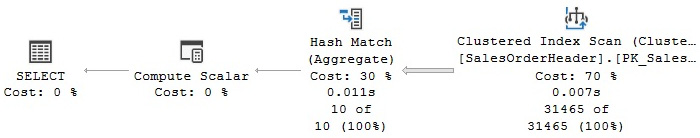
Figure 4.14 – A Hash Aggregate operator

As mentioned earlier, a hash operation builds a hash table in memory. The hash key used for this table is displayed in the Properties window of the Hash Aggregate operator as the Hash Keys Build property, which, in this case, is TerritoryID. Because this table is not sorted by the required column, TerritoryID, every row scanned can belong to any group.

The algorithm for the Hash Aggregate operator is similar to the Stream Aggregate operator, with the exception that, in this case, the input data does not have to be sorted, a hash table is created in memory, and a hash value is calculated for each row that has been processed. For each hash value calculated, the algorithm will check whether a corresponding group already exists in the hash table; if it does not exist, the algorithm will create a new entry for it. In this way, the values for each record are aggregated in this entry on the hash table, and only one row for each group is stored in memory.

Note, again, that a Hash Aggregate operator helps when the data has not been sorted. If you create an index that can provide sorted data, the query optimizer might select a Stream Aggregate operator instead. Run the following statement to create an index, and then execute the previous query again to verify that it uses a Stream Aggregate operator, as shown in Figure 4.15:

CREATE INDEX IX_TerritoryID ON Sales.SalesOrderHeader(TerritoryID)

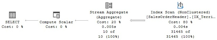
Figure 4.15 – A Stream Aggregate operator using an index

To clean up the changes on the table, drop the index using the following DROP INDEX statement:

DROP INDEX Sales.SalesOrderHeader.IX_TerritoryID

If the input is not sorted and order is explicitly requested in a query, the query optimizer might introduce a Sort operator and a Stream Aggregate operator, as shown earlier. Or it might decide to use a Hash Aggregate operator and then sort the results, as shown in the following query, which produces the plan shown in Figure 4.16. The query optimizer will estimate which operation is the least expensive: sorting the entire input and using a Stream Aggregate operator or using a Hash Aggregate operator and only sorting the aggregated results:

SELECT TerritoryID, COUNT(*)

FROM Sales.SalesOrderHeader

GROUP BY TerritoryID

ORDER BY TerritoryID

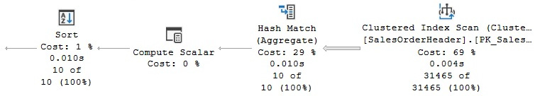
Figure 4.16 – A Hash Aggregate operator followed by a Sort operator

Distinct Sort

Finally, a query using the DISTINCT keyword can be implemented by a Stream Aggregate operator, a Hash Aggregate operator, or a Distinct Sort operator. The Distinct Sort operator is used to both remove duplicates and sort its input. In fact, a query using DISTINCT can be rewritten as a GROUP BY query, and both can generate the same execution plan. If an index to provide sorted data is available, the query optimizer can use a Stream Aggregate operator. If no index is available, SQL Server can introduce a Distinct Sort operator or a Hash Aggregate operator. Let’s look at all three cases here. The following two queries return the same data and produce the same execution plan, as shown in Figure 4.17:

SELECT DISTINCT(JobTitle)

FROM HumanResources.Employee

GO

SELECT JobTitle

FROM HumanResources.Employee

GROUP BY JobTitle

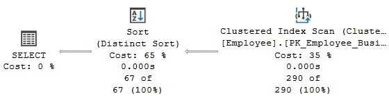
Figure 4.17 – A Distinct Sort operator

Note that the plan is using a Distinct Sort operator. This operator will sort the rows and eliminate any duplicates.

If we create an index, the query optimizer could instead use a Stream Aggregate operator because the plan can take advantage of the fact that the data is already sorted. To test it, run the following CREATE INDEX statement:

CREATE INDEX IX_JobTitle ON HumanResources.Employee(JobTitle)

Then, run the previous two queries again. Both queries will now produce a plan showing a Stream Aggregate operator. Drop the index before continuing by using a DROP INDEX statement:

DROP INDEX HumanResources.Employee.IX_JobTitle

Finally, for a bigger table without an index to provide order, a Hash Aggregate operator can be used, as shown in the two following examples:

SELECT DISTINCT(TerritoryID)

FROM Sales.SalesOrderHeader

GO

SELECT TerritoryID

FROM Sales.SalesOrderHeader

GROUP BY TerritoryID

Both queries produce the same results and will use the same execution plan using a Hash Aggregate operator. Now we will learn about the join operators used by SQL Server.

Joins

In this section, we will talk about the three physical join operators that SQL Server uses to implement logical joins: the Nested Loops Join, Merge Join, and Hash Join operators. It is important to understand that no join algorithm is better than any other and that the query optimizer will select the best join algorithm depending on the specific scenario, as we will explain next.

Nested Loops Join

Let’s start with a query whose purpose is to list employees who are also salespersons. The following query creates the plan shown in Figure 4.18, which uses a Nested Loops Join operator:

SELECT e.BusinessEntityID, TerritoryID

FROM HumanResources.Employee AS e

JOIN Sales.SalesPerson AS s ON e.BusinessEntityID = s.BusinessEntityID

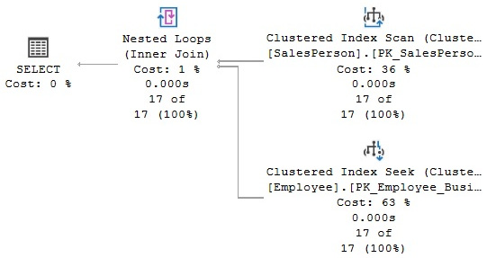
Figure 4.18 – A Nested Loops Join operator

The input shown at the top of the Nested Loops Join plan is known as the outer input, and the one at the bottom is the inner input. The algorithm for the Nested Loops Join operator is very simple: the operator used to access the outer input is executed only once, and the operator used to access the inner input is executed once for every record that qualifies on the outer input. Note that in this example, the plan is scanning the SalesPerson table for the outer input. Because there is no filter on the SalesPerson table, all of its 17 records are returned; therefore, as dictated by the algorithm, the inner input (the Clustered Index Seek operator) is also executed 17 times—once for each row from the outer table.

You can validate this information by looking at the Clustered Index Scan operator properties where you can find the actual number of executions (which, in this case, is 1) and the actual number of rows (which, in this case, is 17). A sample XML fragment is next:

<RelOp EstimateRows="17" PhysicalOp="Clustered Index Scan" … >

  <RunTimeInformation>

    <ActualRows="17" ActualRowsRead="17" ActualExecutions="1" … /> 

  </RunTimeInformation>

</RelOp>

In the same way, the following XML fragment demonstrates that both the actual number of rows and the number of executions are 17:

<RelOp EstimateRows="1" PhisicalOp="Clustered Index Seek" … >

  <RunTimeInformation>

    <ActualRows="17" ActualRowsRead="17" ActualExecutions="17" … /> 

  </RunTimeInformation>

</RelOp>

Let’s change the query to add a filter by TerritoryID:

SELECT e.BusinessEntityID, HireDate

FROM HumanResources.Employee AS e

JOIN Sales.SalesPerson AS s ON e.BusinessEntityID = s.BusinessEntityID

WHERE TerritoryID = 1

This query produces a plan similar to the one shown previously using SalesPerson as the outer input and a Clustered Index Seek operator on the Employee table as the inner input. But this time, the filter on the SalesPerson table is asking for records with TerritoryID equal to 1, and only three records qualify. As a result, the Clustered Index Seek operator, which is the operator on the inner input, is only executed three times. You can verify this information by looking at the properties of each operator, as we did for the previous query.

So, in summary, in the Nested Loops Join algorithm, the operator for the outer input will be executed once and the operator for the inner input will be executed once for every row that qualifies on the outer input. The result of this is that the cost of this algorithm is proportional to the size of the outer input multiplied by the size of the inner input. As such, the query optimizer is more likely to choose a Nested Loops Join operator when the outer input is small, and the inner input has an index on the join key. This join type can be especially effective when the inner input is potentially large, as only a few rows, indicated by the outer input, will be searched.

Merge Join

Now, let’s take a look at a Merge Join example. Run the following query, which produces the execution plan shown in Figure 4.19:

SELECT h.SalesOrderID, s.SalesOrderDetailID, OrderDate

FROM Sales.SalesOrderHeader h

JOIN Sales.SalesOrderDetail s ON h.SalesOrderID = s.SalesOrderID

Figure 4.19 – A Merge Join example

One difference between this and Nested Loops Join is that, in Merge Join, both input operators are only executed once. You can verify this by looking at the properties of both operators, and you’ll find that the number of executions is 1. Another difference is that a Merge Join operator requires an equality operator and its inputs sorted on the join predicate. In this example, the join predicate has an equality operator, which uses the SalesOrderID column, and both clustered indexes are ordered by SalesOrderID.

Benefitting from the fact that both of its inputs are sorted on the join predicate, a Merge Join operator simultaneously reads a row from each input and compares them. If the rows match, they are returned. If the rows do not match, the smaller value can be discarded—because both inputs are sorted, the discarded row will not match any other row on the other input table. This process continues until one of the tables has been completed. Even if there are still rows on the other table, they will clearly not match any rows on the fully scanned table, so there is no need to continue. Because both tables can potentially be scanned, the maximum cost of a Merge Join operator is the sum of scanning both inputs.

If the inputs have not already been sorted, the query optimizer is not likely to choose a Merge Join operator. However, it might decide to sort one or even both inputs if it deems the cost is cheaper than the other alternatives. Let’s follow an exercise to see what happens if we force a Merge Join plan on, for example, a Nested Loops Join plan. If you run the following query, you will notice that it uses a Nested Loops Join operator, as shown in Figure 4.20:

SELECT * FROM Sales.SalesOrderDetail s

JOIN Production.Product p ON s.ProductID = p.ProductID

WHERE SalesOrderID = 43659

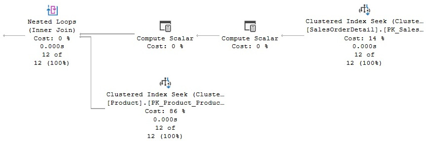
Figure 4.20 – A Nested Loops Join operator

In this case, a good plan is created using efficient Clustered Index Seek operators. If we force a Merge Join operator using a hint, as shown in the following query, the query optimizer has to introduce sorted sources such as Clustered Index Scan and Sort operators, both of which can be seen on the plan shown in Figure 4.21. Of course, these additional operations are more expensive than a Clustered Index Seek operator, and they are only introduced because we instructed the query optimizer to do so:

SELECT * FROM Sales.SalesOrderdetail s

JOIN Production.Product p ON s.ProductID = p.ProductID

WHERE SalesOrderID = 43659

OPTION (MERGE JOIN)

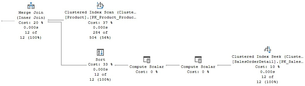
Figure 4.21 – A plan with a hint to use a Merge Join operator

In summary, given the nature of the Merge Join operator, the query optimizer is more likely to choose this algorithm when faced with medium to large inputs, where there is an equality operator on the join predicate, and when the inputs are sorted.

Hash Join

The third join algorithm used by SQL Server is Hash Join. Run the following query to produce the plan displayed in Figure 4.22, and then we’ll take a closer look at the Hash Join operator:

SELECT h.SalesOrderID, s.SalesOrderDetailID FROM Sales.SalesOrderHeader h

JOIN Sales.SalesOrderDetail s ON h.SalesOrderID = s.SalesOrderID

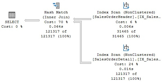
Figure 4.22 – A Hash Join example

In the same way as the Merge Join operator, the Hash Join operator requires an equality operator on the join predicate, but unlike Merge Join, it does not require its inputs to be sorted. In addition, the operations of both inputs are only executed once, which you can verify by looking at the operator properties, as shown earlier. However, a Hash Join operator works by creating a hash table in memory. The query optimizer will use cardinality estimation to detect the smaller of the two inputs, called the build input, and then use it to build a hash table in memory. If there is not enough memory to host the hash table, SQL Server can use a workfile in tempdb, which can impact the performance of the query. A Hash Join operator is a blocking operation, but only during the time the build input is hashed. After the build input has been hashed, the second table, called the probe input, will be read and compared to the hash table using the same mechanism described in the Hash Aggregate section. If the rows are matched, they will be returned, and the results will be streamed through. In the execution plan, the table at the top will be used as the build input and the table at the bottom as the probe input.

Finally, note that a behavior called “role reversal” might appear. If the query optimizer is not able to correctly estimate which of the two inputs is smaller, the build and probe roles may be reversed at execution time, and this will not be shown on the execution plan.

In summary, the query optimizer can choose a Hash Join operator for large inputs where there is an equality operator on the join predicate. Because both tables are scanned, the cost of a Hash Join operator is the sum of scanning both inputs, plus the cost of building the hash table. Now that we have learned about the main joins that we can use in SQL Server, we will explore parallelism, which will help us to run such queries quickly and efficiently.

Parallelism

SQL Server can use parallelism to help execute some expensive queries faster by using several processors simultaneously. However, even when a query might get better performance by using parallel plans, it could still use more resources than a similar serial plan.

For the query optimizer to consider parallel plans, the SQL Server installation must have access to at least two processors or cores or a hyper-threaded configuration. In addition, both the affinity mask and the maximum degree of parallelism advanced configuration options must allow the use of at least two processors, which they do by default. Finally, as explained later in this section, SQL Server will only consider parallelism for serial queries whose cost exceeds the configured cost threshold for parallelism, where the default value is 5.

The affinity mask configuration option specifies which processors are eligible to run SQL Server threads, and the default value of 0 means that all the processors can be used. The maximum degree of the parallelism configuration option is used to limit the number of processors that can be used in parallel plans, and similarly, its default value of 0 allows all available processors to be used. As you can see, if you have the proper hardware, SQL Server allows parallel plans by default, with no additional configuration.

Parallelism will be considered by the query processor when the estimated cost of a serial plan is higher than the value defined in the cost threshold for the parallelism configuration parameter. However, this doesn’t guarantee that parallelism will actually be employed in the final execution plan, as the final decision to parallelize a query (or not) will be based on cost estimations. That is, there is no guarantee that the best parallel plan found will have a lower cost than the best serial plan, so the serial plan might still end up being the selected plan. Parallelism is implemented by the parallelism physical operator, also known as the exchange operator, which implements the Distribute Streams, Gather Streams, and Repartition Streams logical operations.

To create and test parallel plans, we will need to create a couple of large tables in the AdventureWorks2019 database. One of these tables will also be used in the next section. A simple way to do this is to copy the data from Sales.SalesOrderDetail a few times by running the following statements:

SELECT *

INTO #temp

FROM Sales.SalesOrderDetail

UNION ALL SELECT * FROM Sales.SalesOrderDetail

UNION ALL SELECT * FROM Sales.SalesOrderDetail

UNION ALL SELECT * FROM Sales.SalesOrderDetail

UNION ALL SELECT * FROM Sales.SalesOrderDetail

UNION ALL SELECT * FROM Sales.SalesOrderDetail

SELECT IDENTITY(int, 1, 1) AS ID, CarrierTrackingNumber, OrderQty, ProductID,

UnitPrice, LineTotal, rowguid, ModifiedDate

INTO dbo.SalesOrderDetail FROM #temp

SELECT IDENTITY(int, 1, 1) AS ID, CarrierTrackingNumber, OrderQty, ProductID,

UnitPrice, LineTotal, rowguid, ModifiedDate

INTO dbo.SalesOrderDetail2 FROM #temp

DROP TABLE #temp

The following query, using one of the tables we just created, will produce a parallel plan. Because this plan is too big to print in this book, only part of it is displayed in Figure 4.23:

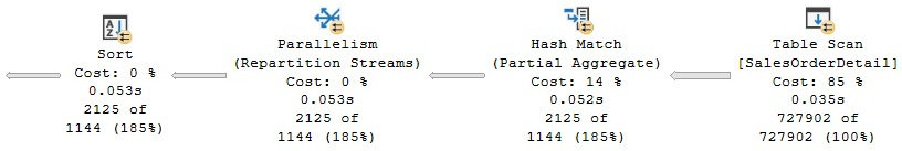
Figure 4.23 – Part of a parallel plan

SELECT ProductID, COUNT(*)

FROM dbo.SalesOrderDetail

GROUP BY ProductID

One benefit of the graphical plans, compared to the text and XML plans, is that you can easily see which operators are being executed in parallel by looking at the parallelism symbol (a small yellow circle with arrows) included in the operator icon.

To see why a parallel plan was considered and selected, you can look at the cost of the serial plan. One way to do this is by using the MAXDOP hint to force a serial plan on the same query, as shown next:

SELECT ProductID, COUNT(*)

FROM dbo.SalesOrderDetail

GROUP BY ProductID

OPTION (MAXDOP 1)

The forced serial plan has a cost of 9.70746. Given that the default cost threshold for the parallelism configuration option is 5, this crosses that threshold. An interesting test you can perform in your test environment is to change the cost threshold for the parallelism option to 10 by running the following statements:

EXEC sp_configure 'cost threshold for parallelism', 10

GO

RECONFIGURE

GO

If you run the same query again, this time without the MAXDOP hint, you will get a serial plan with a cost of 9.70746. Because the cost threshold for parallelism is now 10, the query optimizer did not even try to find a parallel plan. If you have followed this exercise, do not forget to change the cost threshold for the parallelism configuration option back to the default value of 5 by running the following statement:

EXEC sp_configure 'cost threshold for parallelism', 5

GO

RECONFIGURE

GO

The exchange operator

As mentioned earlier, parallelism is implemented by the parallelism physical operator, which is also known as the exchange operator. Parallelism in SQL Server works by splitting a task among two or more copies of the same operator, each copy running in its own scheduler. For example, if you were to ask SQL Server to count the number of records on a small table, it might use a single Stream Aggregate operator to do that. But if you request it to count the number of records in a very large table, SQL Server might use two or more Stream Aggregate operators, with each counting the number of records of a part of the table. These Stream Aggregate operators would run in parallel, each one in a different scheduler and each performing part of the work. This is a simplified explanation, but this section will explain the details.

In most cases, the actual partitioning of data between these operators is handled by the parallelism or exchange operator. Interestingly, most of these operators do not need to be aware that they are being executed in parallel. For example, the Stream Aggregate operator we just mentioned only receives records, counts them, and then returns the results without knowing that other Stream Aggregate operators are also performing the same operation with distinct records of a table. Of course, there are also parallel-aware operators such as Parallel Scan, which we will cover next. To see how it works, run the next query, which creates the parallel plan shown in Figure 4.24:

SELECT * FROM dbo.SalesOrderDetail

WHERE LineTotal > 3234

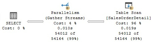
Figure 4.24 – A Parallel Scan query

As mentioned earlier, Parallel Scan is one of the few parallel-aware operators in SQL Server and is based on the work performed by the parallel page supplier, a storage engine process that assigns sets of pages to operators in the plan. In the plan shown, SQL Server will assign two or more Table Scan operators, and the parallel page supplier will provide them with sets of pages. One great advantage of this method is that it does not need to assign an equal number of pages per thread. However, they are assigned on demand, which could help in cases where one CPU might be busy with some other system activities and might not be able to process many records; thus, it does not slow down the entire process. For example, in my test execution, I see two threads—one processing 27,477 and the other 26,535 rows, as shown in the following XML plan fragment (you can also see this information on the graphical plan by selecting the properties of the Table Scan operator and expanding the Actual Number of Rows section):

<RunTimeInformation>

<RunTimeCountersPerThread Thread="1" ActualRows="27477" … />

<RunTimeCountersPerThread Thread="2" ActualRows="26535" … />

<RunTimeCountersPerThread Thread="0" ActualRows="0" … />

</RunTimeInformation>

But of course, this depends on the activity of each CPU. To simulate this, we ran another test while one of the CPUs was busy, and the plan showed one thread processing only 11,746 rows, while the second was processing 42,266. Notice that the plan also shows thread 0, which is the coordinator or main thread, and does not process any rows.

Although the plan in Figure 4.24 only shows a Gather Streams exchange operator, the exchange operator can take two additional functions or logical operations as Distribute Streams and Repartition Stream exchange operators.

A Gather Streams exchange is also called a start parallelism exchange, and it is always at the beginning of a parallel plan or region, considering that execution starts from the far left of the plan. This operator consumes several input streams, combines them, and produces a single output stream of records. For example, in the plan shown in Figure 4.24, the Gather Streams exchange operator consumes the data produced by the two Table Scan operators running in parallel and sends all of these records to its parent operator.

Opposite to a Gather Streams exchange, a Distribute Streams exchange is called a stop parallelism exchange. It takes a single input stream of records and produces multiple output streams. The third exchange logical operation is the Repartition Streams exchange, which can consume multiple streams and produce multiple streams of records.

In the previous example, we saw that Parallel Scan is a parallel-aware operator in which the parallel page supplier assigns sets of pages to operators in the plan. As indicated earlier, most of the time, operators are not aware they are running in parallel, and so it is the job of the exchange operator to send them rows using one of the partitioning types shown in Table 4.2:

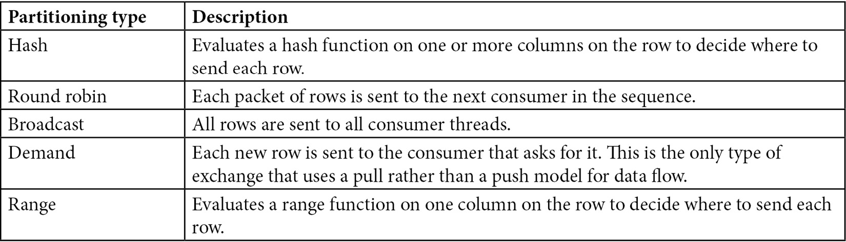
Table 4.2 – Types of partitioning

These types of partitioning are exposed to the user in the Partitioning Type property of execution plans, and they only make sense for Repartition Streams and Distribute Streams exchanges because, as shown in Figure 4.24, a Gather Streams exchange only routes the rows to a single consumer thread. A couple of examples of partitioning types will be shown later in this section.

Finally, another property of the exchange operators is that they preserve the order of the input rows. When they do this, they are called merging or order-preserving exchanges. Otherwise, they are called non-merging or non-order-preserving exchanges. Merging exchanges do not perform any sort operation; rows must be already in sorted order. Because of this, this order-preserving operation only makes sense for Gather Streams and Repartition Streams exchanges. With a Distribute Streams exchange, there is only one producer, so there is nothing to merge. However, it is also worth mentioning that merging exchanges might not scale as well as non-merging exchanges. For example, compare the execution plans of these two versions of the first example in this section, the second one using an ORDER BY clause:

SELECT ProductID, COUNT(*)

FROM dbo.SalesOrderDetail

GROUP BY ProductID

GO

SELECT ProductID, COUNT(*)

FROM dbo.SalesOrderDetail

GROUP BY ProductID

ORDER BY ProductID

Although both plans are almost the same, the second one returns results that have been sorted by using an order-preserving exchange operator. You can verify that by looking at the properties of the Gather Streams exchange operator in a graphical plan, which includes an Order By section. This is also shown in the following XML fragment:

<RelOp LogicalOp="Gather Streams" PhysicalOp="Parallelism" … >

  <Parallelism>

    <OrderBy>

      <OrderByColumn Ascending="true">

        <ColumnReference … Column="ProductID" />

      </OrderByColumn>

    </OrderBy>

Hash partitioning is the most common partitioning type and can be used to parallelize a Merge Join operator or a Hash Join operator, such as in the following example. Run the next query, which will get the plan shown in Figure 4.25:

SELECT * FROM dbo.SalesOrderDetail s1 JOIN dbo.SalesOrderDetail2 s2

ON s1.id = s2.id

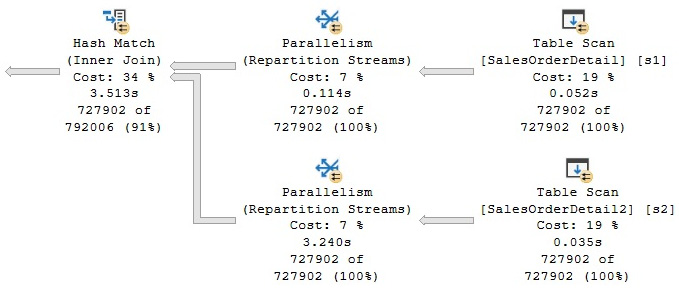
Figure 4.25 – A hash partitioning example

Although not shown here, you can validate that hash partitioning is being used by the Repartition Streams exchanges by looking at the Partitioning Type property of one of these operators in a graphical plan. This is shown in the following XML plan fragment. In this case, hash partitioning distributes the build and probe rows among the individual Hash Join threads:

<RelOp LogicalOp="Repartition Streams" PhysicalOp="Parallelism" … >

  <Parallelism PartitioningType="Hash">

Finally, the following query, which includes a very selective predicate, produces the plan in Figure 4.26 and shows both a start parallelism operator or a Gather Streams exchange and a stop parallelism operator or a Distribute Streams exchange:

SELECT * FROM dbo.SalesOrderDetail s1

JOIN dbo.SalesOrderDetail2 s2 ON s1.ProductID = s2.ProductID

WHERE s1.id = 123

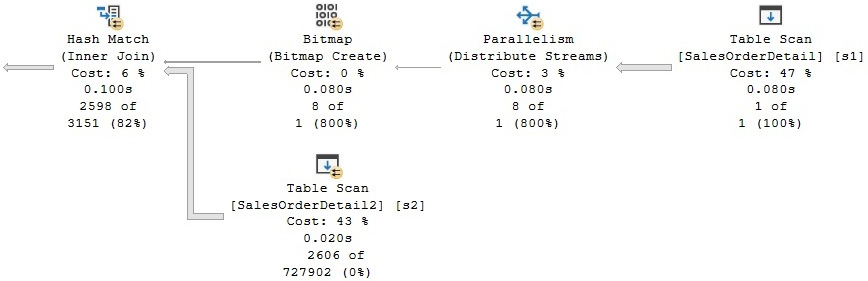
Figure 4.26 – A broadcast partitioning example

The Distribute Streams exchange operator uses broadcast partitioning, as you can verify from the properties of the operator in a graphical plan (look for the partitioning type of Broadcast) and also shown in the following XML fragment. Broadcast partitioning sends the only row that qualifies from table1 to all the Hash Join threads. Additionally, a bitmap operator is used to eliminate most of the rows from table2, which greatly improves the performance of the query:

<RelOp LogicalOp="Distribute Streams" PhysicalOp="Parallelism" … >

  <Parallelism PartitioningType="Broadcast">

We will cover bitmap operators in more detail in Chapter 11, An Introduction to Data Warehouses, where you will see how they are used to optimize the performance of data warehouse queries.

Limitations

You might see cases when you have an expensive query that is not parallelized. There are several SQL Server features that can inhibit a parallel plan from creating a serial plan instead:

• Scalar-valued user-defined functions
• CLR user-defined functions with data access
• Miscellaneous built-in functions such as OBJECT_ID(), ERROR_NUMBER(), and @@TRANCOUNT
• Dynamic cursors

Similarly, there are some other features that force a serial zone within a parallel plan, which can lead to performance problems. These features include the following:

• Multistatement, table-valued, and user-defined functions
• TOP clauses
• Global scalar aggregates
• Sequence functions
• Multiconsumer spools
• Backward scans
• System table scans
• Recursive queries

For example, the following code shows how the first parallel example in this section turns into a serial plan while using a simple user-defined function:

CREATE FUNCTION dbo.ufn_test(@ProductID int)

RETURNS int

AS

BEGIN

RETURN @ProductID

END

GO

SELECT dbo.ufn_test(ProductID), ProductID, COUNT(*)

FROM dbo.SalesOrderDetail

GROUP BY ProductID

As covered in Chapter 1, An Introduction to Query Tuning and Optimization, the NonParallelPlanReason optional attribute of the QueryPlan element contains a high-level description of why a parallel plan might not be chosen for the optimized query, which in this case is CouldNotGenerateValidParallelPlan, as shown in the following XML plan fragment:

<QueryPlan … NonParallelPlanReason="CouldNotGenerateValidParallelPlan" … >

There is an undocumented and, therefore, unsupported trace flag that you could try to force a parallel plan. Trace flag 8649 can be used to set the cost overhead of parallelism to 0, encouraging a parallel plan, which could help in some cases (mostly cost-related). As mentioned earlier, an undocumented trace flag must not be used in a production environment. Just for demonstration purposes, see the following example using a small table (note it is the SalesOrderDetail table in the Sales schema, not the bigger table in the dbo schema that we created earlier):

SELECT ProductID, COUNT(*)

FROM Sales.SalesOrderDetail

GROUP BY ProductID

The previous query creates a serial plan with a cost of 0.429621. Using trace flag 8649, as shown next, we will create a parallel plan with a slightly lower cost of 0.386606 units:

SELECT ProductID, COUNT(*)

FROM Sales.SalesOrderDetail

GROUP BY ProductID

OPTION (QUERYTRACEON 8649)

So far, we have focused on how the query processor solves SELECT queries, so in the next and last section, we will talk about update operations.

Updates

Update operations are an intrinsic part of database operations, but they also need to be optimized so that they can be performed as quickly as possible. In this section, bear in mind that when we say “updates,” in general, we are referring to any operation performed by the INSERT, DELETE, and UPDATE statements, as well as the MERGE statement, which was introduced in SQL Server 2008. In this chapter, I explain the basics of update operations and how they can quickly become complicated, as they need to update existing indexes, access multiple tables, and enforce existing constraints. We will see how the query optimizer can select per-row and per-index plans to optimize UPDATE statements. Additionally, we will describe the Halloween protection problem and how SQL Server avoids it.

Even when performing an update that involves some other areas of SQL Server, such as a transaction, concurrency control, or locking, update operations are still totally integrated within the SQL Server query processor framework. Also, update operations are optimized so that they can be performed as quickly as possible. So, in this section, I will talk about updates from a query-processing point of view. As mentioned earlier, for this section, we refer to any operations performed by the INSERT, DELETE, UPDATE, and MERGE statements as “updates.”

Update plans can be complicated because they need to update existing indexes alongside data. Also, because of objects such as check constraints, referential integrity constraints, and triggers, those plans might have to access multiple tables and enforce existing constraints. Updates might also require the updating of multiple tables when cascading referential integrity constraints or triggers are defined. Some of these operations, such as updating indexes, can have a big impact on the performance of the entire update operation, and we will take a deeper look at that now.

Update operations are performed in two steps, which can be summarized as a read section followed by the update section. The first step provides the details of the changes to apply and which records will be updated. For INSERT operations, this includes the values to be inserted, and for DELETE operations, it includes obtaining the keys of the records to be deleted, which could be the clustering keys for clustered indexes or the RIDs for heaps. However, for update operations, a combination of both the keys of the records to be updated and the data to be inserted is needed. In this first step, SQL Server might read the table to be updated, just like in any other SELECT statement. In the second step, the update operations are performed, including updating indexes, validating constraints, and executing triggers. The entire update operation will fail and roll back if it violates any defined constraint.

Let’s start with an example of a very simple update operation. Inserting a new record on the Person.CountryRegion table using the following query creates a very simple plan, as shown in Figure 4.27:

INSERT INTO Person.CountryRegion (CountryRegionCode, Name)

VALUES ('ZZ', 'New Country')

Figure 4.27 – An insert example

However, the operation gets complicated very quickly when you try to delete the same record by running the following statement, as shown in Figure 4.28:

DELETE FROM Person.CountryRegion

WHERE CountryRegionCode = 'ZZ'

Figure 4.28 – A delete example

As you can see in the preceding plan, in addition to CountryRegion, three additional tables (StateProvince, CountryRegionCurrency, and SalesTerritory) are accessed. The reason behind this is that these three tables have foreign keys referencing CountryRegion, so SQL Server needs to validate that no records exist on these tables for this specific value of CountryRegionCode. Therefore, the tables are accessed and an Assert operator is included at the end of the plan to perform this validation. If a record with the CountryRegionCode value to be deleted exists in any of these tables, the Assert operator will throw an exception and SQL Server will roll back the transaction, returning the following error message:

Msg 547, Level 16, State 0, Line 1

The DELETE statement conflicted with the REFERENCE constraint

"FK_CountryRegionCurrency_CountryRegion_CountryRegionCode". The conflict occurred in database "AdventureWorks2019", table "Sales.CountryRegionCurrency", column 'CountryRegionCode'.

The statement has been terminated.

As you can see, the preceding example shows how update operations can access some other tables not included in the original query—in this case, because of the definition of referential integrity constraints. The updating of nonclustered indexes is covered in the next section.

Per-row and per-index plans

An important operation performed by updates is the modifying and updating of existing nonclustered indexes, which is done by using per-row or per-index maintenance plans (also called narrow and wide plans, respectively). In a per-row maintenance plan, the updates to the base table and the existing indexes are performed by a single operator, one row at a time. On the other hand, in a per-index maintenance plan, the base table and each nonclustered index are updated in separate operations.

Except for a few cases where per-index plans are mandatory, the query optimizer can choose between a per-row plan and a per-index plan based on performance reasons, and an index-by-index basis. Although factors such as the structure and size of the table, along with the other operations performed by the update statement, are all considered, choosing between per-index and per-row plans will mostly depend on the number of records being updated. The query optimizer is more likely to choose a per-row plan when a small number of records is being updated, and a per-index plan when the number of records to be updated increases because this choice scales better. A drawback with the per-row approach is that the storage engine updates the nonclustered index rows using the clustered index key order, which is not efficient when a large number of records needs to be updated.

The following DELETE statement will create a per-row plan, which is shown in Figure 4.29. Some additional queries might be shown on the plan due to the execution of an existing trigger.

Note

In this section, two queries update data from the AdventureWorks2019 database, so perhaps you should request an estimated plan if you don’t want the records to be updated. Also, the BEGIN TRANSACTION and ROLLBACK TRANSACTION statements can be used to create and roll back the transaction. Alternatively, you could perform the updates and later restore a fresh copy of the AdventureWorks2019 database.

DELETE FROM Sales.SalesOrderDetail

WHERE SalesOrderDetailID = 61130

Figure 4.29 – A per-row plan

In addition to updating the clustered index, this delete operation will update two existing nonclustered indexes, IX_SalesOrderDetail_ProductID and AK_SalesOrderDetail_rowguid, which you can verify by looking at the properties of the Clustered Index Delete operator.

To see a per-index plan, we need a table with a large number of rows, so we will be using the dbo.SalesOrderDetail table that we created in the Parallelism section. Let’s add two nonclustered indexes to the table by running the following statements:

CREATE NONCLUSTERED INDEX AK_SalesOrderDetail_rowguid

ON dbo.SalesOrderDetail (rowguid)

CREATE NONCLUSTERED INDEX IX_SalesOrderDetail_ProductID

ON dbo.SalesOrderDetail (ProductID)

As indicated earlier, when a large number of records is being updated, the query optimizer might choose a per-index plan, which the following query will demonstrate, by creating the per-index plan shown in Figure 4.30:

DELETE FROM dbo.SalesOrderDetail WHERE ProductID < 953

Figure 4.30 – A per-index plan

In this per-index update plan, the base table is updated using a Table Delete operator, while a Table Spool operator is used to read the data of the key values of the indexes to be updated and a Sort operator sorts the data in the order of the index. In addition, an Index Delete operator updates a specific nonclustered index in one operation (the name of which you can see in the properties of each operator). Although the table spool is listed twice in the plan, it is the same operator being reused. Finally, the Sequence operator makes sure that each Index Delete operation is performed in sequence, as shown from top to bottom.

You can now delete the tables you have created for these exercises by using the following DROP TABLE statements:

DROP TABLE dbo.SalesOrderDetail

DROP TABLE dbo.SalesOrderDetail2

For demonstration purposes only, you could use the undocumented and unsupported trace flag, 8790, to force a per-index plan on a query, where the number of records being updated is not large enough to produce this kind of plan. For example, the following query on Sales.SalesOrderDetail requires this trace flag to produce a per-index plan; otherwise, a per-row plan will be returned instead:

DELETE FROM Sales.SalesOrderDetail

WHERE SalesOrderDetailID < 43740

OPTION (QUERYTRACEON 8790)

In summary, bear in mind that, except for a few cases where per-index plans are mandatory, the query optimizer can choose between a per-row plan and a per-index plan on an index-by-index basis, so it is even possible to have both maintenance choices in the same execution plan.

Finally, we close this chapter by covering an interesting behavior of update operations, called Halloween protection.

Halloween protection

Halloween protection refers to a problem that appears in certain update operations and was discovered more than 30 years ago by researchers working on the System R project at the IBM Almaden Research Center. The System R team was testing a query optimizer when they ran a query to update the salary column on an Employee table. The UPDATE statement was supposed to give a 10 percent raise to every employee with a salary of less than $25,000.

Even when there were salaries considerably lower than $25,000, to their surprise, no employee had a salary under $25,000 after the update query was completed. They noticed that the query optimizer had selected an index based on the salary column and had updated some records multiple times until they reached the $25,000 salary value. Because the salary index was used to scan the records, when the salary column was updated, some records were moved within the index and were then scanned again later, so those records were updated more than once. The problem was called the Halloween problem because it was discovered on Halloween day, probably in 1976 or 1977.

As I mentioned at the beginning of this section, update operations have a read section followed by an update section, and that is a crucial distinction to bear in mind at this stage. To avoid the Halloween problem, the read and update sections must be completely separated; the read section must be completed in its entirety before the write section is run. In the next example, we will show you how SQL Server avoids the Halloween problem. Run the following statement to create a new table:

SELECT * INTO dbo.Product FROM Production.Product

Run the following UPDATE statement, which produces the execution plan shown in Figure 4.31:

UPDATE dbo.Product SET ListPrice = ListPrice * 1.2

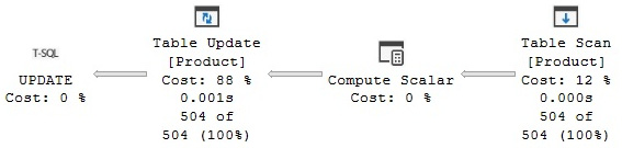
Figure 4.31 – An update without Halloween protection

In this case, no Halloween protection is needed because the statement updates the ListPrice column, which is not part of any index, so updating the data does not move any rows around. Now, to demonstrate the problem, let’s create a clustered index on the ListPrice column, by running the following statement:

CREATE CLUSTERED INDEX CIX_ListPrice ON dbo.Product(ListPrice)

Run the preceding UPDATE statement again. The query will show a similar plan, but this time including a Table Spool operator, which is a blocking operator, separating the read section from the write section. A blocking operator has to read all of the relevant rows before producing any output rows for the next operator. In this example, the table spool separates the Clustered Index Scan operator from the Clustered Index Update operator, as shown in Figure 4.32:

Figure 4.32 – An update with Halloween protection

The spool operator scans the original data and saves a copy of it in a hidden spool table in tempdb before it is updated. Generally, a Table Spool operator is used to avoid the Halloween problem because it is a cheap operator. However, if the plan already includes another operator that can be used, such as Sort, then the Table Spool operator is not needed, and the Sort operator can perform the same blocking job instead.

Finally, drop the table you have just created:

DROP TABLE dbo.Product

Summary

In this chapter, we described the execution engine as a collection of physical operators, which also defines the choices that are available for the query optimizer to build execution plans with. Some of the most commonly used operators of the execution engine were introduced, including their algorithms, relative costs, and the scenarios in which the query optimizer is more likely to choose them. In particular, we looked at operators for data access, aggregations, joins, parallelism, and update operations.

Also, the concepts of sorting and hashing were introduced as a mechanism used by the execution engine to match and process data. Data access operations included the scanning of tables and indexes, the index seeks, and bookmark lookup operations. Aggregation algorithms such as Stream Aggregate and Hash Aggregate were discussed, along with join algorithms such as the Nested Loops Join, Merge Join, and Hash Join operators. Additionally, an introduction to parallelism was presented, closing the chapter with update topics such as per-row and per-index plans and Halloween protection.

Understanding how these operators work, along with what they are likely to cost, will give you a much stronger sense of what is happening under the hood when you investigate how your queries are being executed. In turn, this will help you to find potential problems in your execution plans and to understand when to resort to any of the techniques we describe later in the book..