
Chapter 3: The Query Optimizer
In this chapter, we will cover how the SQL Server Query Optimizer works and introduce the steps it performs in the background. This covers everything, from the time a query is submitted to SQL Server until an execution plan is generated and is ready to be executed. This includes steps such as parsing, binding, simplification, trivial plan optimization, and full optimization. Important components and mechanisms that are part of the Query Optimizer architecture, such as transformation rules and the Memo structure, are also introduced.
The purpose of the Query Optimizer is to provide an optimum execution plan, or at least a good enough execution plan, and to do so, it generates many possible alternatives through the use of transformation rules. These alternative plans are stored for the duration of the optimization process in a structure called the Memo. Unfortunately, a drawback of cost-based optimization is the cost of optimization itself. Given that finding the optimum plan for some queries would take an unacceptably long optimization time, some heuristics are used to limit the number of alternative plans considered instead of using the entire search space—remember that the goal is to find a good enough plan as quickly as possible. Heuristics help the Query Optimizer to cope with the combinatorial explosion that occurs in the search space as queries get progressively more complex. However, the use of transformation rules and heuristics does not necessarily reduce the cost of the available alternatives, so the cost of each candidate plan is also determined, and the best alternative is chosen based on those costs.
This chapter covers the following topics:
- Query optimization research
- Introduction to query processing
- The sys.dm_exec_query_optimizer_info DMV
- Parsing and binding
- Simplification
- Trivial plan
- Joins
- Transformation rules
- The memo
- Statistics
- Full optimization
Query optimization research
Query optimization research dates back to the early 1970s. One of the earliest works describing a cost-based query optimizer was Access Path Selection in a Relational Database Management System, published in 1979 by Pat Selinger et al, to describe the query optimizer for an experimental database management system developed in 1975 at what is now the IBM Almaden Research Center. This database management system, called System R, advanced the field of query optimization by introducing the use of cost-based query optimization, the use of statistics, an efficient method of determining join orders, and the addition of CPU cost to the optimizer’s cost estimation formulae.
Yet, despite being an enormous influence in the field of query optimization research, it suffered a major drawback: its framework could not be easily extended to include additional transformations. This led to the development of more extensible optimization architectures that facilitated the gradual addition of new functionality to query optimizers. The trailblazers in this field were the Exodus Optimizer Generator, defined by Goetz Graefe and David DeWitt, and, later, the Volcano Optimizer Generator, defined by Goetz Graefe and William McKenna. Goetz Graefe then went on to define the Cascades Framework, resolving errors that were present in his previous two endeavors.
What is most relevant for us about this previous research is that SQL Server implemented a new cost-based query optimizer, based on the Cascades Framework, in 1999, when its database engine was re-architected for the release of SQL Server 7.0. The extensible architecture of the Cascades Framework has made it much easier for new functionality, such as new transformation rules or physical operators, to be implemented in the Query Optimizer. We will now check out the what and how of query processing.
Introduction to query processing
The query optimization and execution process was introduced in Chapter 1, An Introduction to Query Tuning and Optimization, and will be explained in more detail throughout this chapter. However, before we get started, we’ll briefly explore the inner workings of the query optimization process, which extends both before and after the Query Optimizer itself. The diagram in Figure 3.1 shows the major phases of the query processing process, and each phase will be explained in more detail in the remaining sections of this chapter.
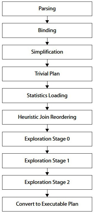
Figure 3.1 – The query-processing process
Parsing and binding are the first operations performed when a query is submitted to a SQL Server database engine. Parsing and binding produce a tree representation of the query, which is then sent to the Query Optimizer to perform the optimization process. At the beginning of this optimization process, this logical tree will be simplified, and the Query Optimizer will check whether the query qualifies for a trivial plan. If it does, a trivial execution plan is returned and the optimization process immediately ends. The parsing, binding, simplification, and trivial plan processes do not depend on the contents of the database (such as the data itself), but only on the database schema and query definition. Because of this, these processes also do not use statistics, cost estimation, or cost-based decisions, all of which are only employed during the full optimization process.
If the query does not qualify for a trivial plan, the Query Optimizer will run the full optimization process, which is executed in up to three stages, and a plan may be produced at the end of any of these stages. In addition, to consider all of the information gathered in the previous phases, such as the query definition and database schema, the full optimization process will use statistics and cost estimation and will then select the best execution plan (within the available time) based solely on that plan’s cost
The Query Optimizer has several optimization phases designed to try to optimize queries as quickly and simply as possible and to not use more expensive and sophisticated options unless absolutely necessary. These phases are called the simplification, trivial plan optimization, and full optimization stages. In the same way, the full optimization phase itself consists of up to three stages, as follows:
- Transaction processing
- Quick plan
- Full optimization phases
These three stages are also simply called search 0, search 1, and search 2 phases, respectively. Plans can be produced in any of these stages, except for the simplification phase, which we will discuss in a moment.
Caution
This chapter contains many undocumented and unsupported features, and they are identified in each section as such. They are included in the book and intended for educational purposes so you can use them to better understand how the Query Optimizer works. These undocumented and unsupported features are not supposed to be used in a production environment. Use them carefully, if possible, and only on your own isolated non-production SQL Server instance.
Now that we have explored query processing, we will now check out a unique DMV that can be used for more insights about the Query Optimizer.
The sys.dm_exec_query_optimizer_info DMV
You can use the sys.dm_exec_query_optimizer_info DMV to gain additional insight into the work being performed by the Query Optimizer. This DMV, which is only partially documented, provides information regarding the optimizations performed on the SQL Server instance. Although this DMV contains cumulative statistics recorded since the given SQL Server instance was started, it can also be used to get optimization information for a specific query or workload, as we’ll see in a moment.
As mentioned, you can use this DMV to obtain statistics regarding the operation of the Query Optimizer, such as how queries have been optimized and how many of them have been optimized since the instance started. This DMV returns three columns:
- Counter: The name of the optimizer event
- Occurrence: The number of occurrences of the optimization event for this counter
- Value: The average value per event occurrence
Thirty-eight counters were originally defined for this DMV when it was originally introduced with SQL Server 2005, and a new counter called merge stmt was added in SQL Server 2008, giving a total of 39, which continues through SQL Server 2022. To view the statistics for all the query optimizations since the SQL Server instance was started, we can just run the following:
SELECT * FROM sys.dm_exec_query_optimizer_info
Here is the partial output we get from one production instance:

The output shows that there have been 691,473 optimizations since the instance was started, that the average elapsed time for each optimization was 0.0078 seconds, and that the average estimated cost of each optimization, in internal cost units, was about 1.398. This particular example shows optimizations of inexpensive queries typical of an OLTP system.
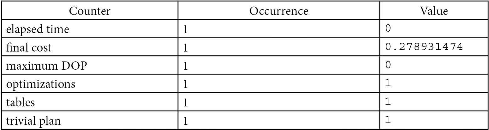
Although the sys.dm_exec_query_optimizer_info DMV was completely documented in the original version of SQL Server 2005 documentation (originally called Books Online), more recent versions of the documentation omit descriptions of nearly half (18 out of 39) of the counters, and instead label them as Internal only. Therefore, in Table 3.1, you can see the currently documented descriptions plus descriptions of the 18 undocumented counters, according to their original documentation, which is still valid for SQL Server 2022:
.jpg)
.jpg)
.jpg)
Table 3.1 – The sys.dm_exec_query_optimizer_info DMV with undocumented counters
The counters can be used in several ways to show important insights about the optimizations being performed in your instance. For example, the next query displays the percentage of optimizations in the instance that includes hints. This information could be useful to show how extensive the use of hints in your databases is, which in turn can demonstrate that your code may be less flexible than anticipated and may require additional maintenance. Hints are explained in detail in the last chapter of this book. Table 3.1 showcases the various counters, which we can find out using the following code as well:
SELECT (SELECT occurrence FROM sys.dm_exec_query_optimizer_info WHERE counter =
‘hints’) * 100.0 / (SELECT occurrence FROM sys.dm_exec_query_optimizer_info
WHERE counter = ‘optimizations’)
As mentioned previously, you can use this DMV in two different ways: you can use it to get information regarding the history of accumulated optimizations on the system since the instance was started, or you can use it to get optimization information for a particular query or a workload. To capture data on the latter, you need to take two snapshots of the DMV—one before optimizing your query and another one after the query has been optimized—and manually find the difference between them. Unfortunately, there is no way to initialize the values of this DMV, which could make this process easier.
However, there may still be several issues to consider when capturing two snapshots of this DMV. First, you need to eliminate the effects of system-generated queries and queries executed by other users that may be running at the same time as your sample query. Try to isolate the query or workload on your own instance, and make sure that the number of optimizations reported is the same as the number of optimizations you are requesting to optimize by checking the optimizations counter. If the former is greater, the data probably includes some of those queries submitted by the system or other users. Of course, it’s also possible that your own query against the sys.dm_exec_query_optimizer_info DMV may count as an optimization.
Second, you need to make sure that query optimization is actually taking place. For example, if you run the same query more than once, SQL Server may simply use an existing plan from the plan cache, without performing any query optimization. You can force an optimization by using the RECOMPILE hint (as shown later), using sp_recompile, or by manually removing the plan from the plan cache. For instance, starting with SQL Server 2008, the DBCC FREEPROCCACHE statement can be used to remove a specific plan, all the plans related to a specific resource pool, or the entire plan cache. It is worth warning you at this point not to run commands to clear the entire plan cache of a production environment.
With all of this in mind, the script shown next will display the optimization information for a specific query, while avoiding all the aforementioned issues. The script has a section to include the query you want the optimization information from:
-- optimize these queries now
-- so they do not skew the collected results
GO
SELECT *
INTO after_query_optimizer_info
FROM sys.dm_exec_query_optimizer_info
GO
SELECT *
INTO before_query_optimizer_info
FROM sys.dm_exec_query_optimizer_info
GO
DROP TABLE before_query_optimizer_info
DROP TABLE after_query_optimizer_info
GO
-- real execution starts
GO
SELECT *
INTO before_query_optimizer_info
FROM sys.dm_exec_query_optimizer_info
GO
-- insert your query here
SELECT *
FROM Person.Address
-- keep this to force a new optimization
OPTION (RECOMPILE)
GO
SELECT *
INTO after_query_optimizer_info
FROM sys.dm_exec_query_optimizer_info
GO
SELECT a.counter,
(a.occurrence - b.occurrence) AS occurrence,
(a.occurrence * a.value - b.occurrence *
b.value) AS value
FROM before_query_optimizer_info b
JOIN after_query_optimizer_info a
ON b.counter = a.counter
WHERE b.occurrence <> a.occurrence
DROP TABLE before_query_optimizer_info
DROP TABLE after_query_optimizer_info
Note that some queries are listed twice in the code. The purpose of this is to optimize them the first time they are executed so that their plan can be available in the plan cache for all the executions after that. In this way, we aim as far as possible to isolate the optimization information from the queries we are trying to analyze. Care must be taken that both queries are exactly the same, including case, comments, and so on, and separated in their own batch for the GO statements.
If you run this script against the AdventureWorks2019 database, the output (after you have scrolled past the output of your query) should look like what is shown next. Note that the times shown obviously may be different from the ones you get in your system, for both this and other examples in this chapter. The output indicates, among other things, that there was one optimization, referencing one table, with a cost of 0.278931474:
Certainly, for this simple query, we could find the same information in some other places, such as in an execution plan. However, as I will show later in this chapter, this DMV can provide optimization information that is not available anywhere else. I will be using this DMV later in this chapter to show you why it is very useful in providing additional insight into the work being performed by the Query Optimizer. With that, we will move on to two of the initial operations that SQL Server executes when you query it.
Parsing and binding
Parsing and binding are the first operations that SQL Server executes when you submit a query to the database engine and are performed by a component called the Algebrizer. Parsing first makes sure that the Transact-SQL (T-SQL) query has a valid syntax and then uses the query information to build a tree of relational operators. By that, I mean the parser translates the SQL query into an algebra tree representation of logical operators, which is called a parse tree. Parsing only checks for valid T-SQL syntax, not for valid table or column names, which are verified in the next phase: binding.
Parsing is similar to the Parse functionality available in Management Studio (by clicking the Parse button on the default toolbar) or the SET PARSEONLY statement. For example, the following query will successfully parse on the AdventureWorks2019 database, even when the listed columns and table do not exist in the said database:
SELECT lname, fname FROM authors
However, if you incorrectly write the SELECT or FROM keyword, like in the next query, SQL Server will return an error message complaining about the incorrect syntax:
SELECT lname, fname FRXM authors
Once the parse tree has been constructed, the Algebrizer performs the binding operation, which is mostly concerned with name resolution. During this operation, the Algebrizer makes sure that all of the objects named in the query do actually exist, confirms that the requested operations between them are valid, and verifies that the objects are visible to the user running the query (in other words, the user has the proper permissions). It also associates every table and column name on the parse tree with their corresponding object in the system catalog. Name resolution for views includes the process of view substitution, where a view reference is expanded to include the view definition—for example, to directly include the tables used in the view. The output of the binding operation, which is called an algebrizer tree, is then sent to the Query Optimizer, as you’ll have guessed, for optimization.
Originally, this tree will be represented as a series of logical operations that are closely related to the original syntax of the query. These include such logical operations as get data from the Customer table, get data from the Contact table, perform an inner join, and so on. Different tree representations of the query will be used throughout the optimization process, and this logical tree will receive different names until it is finally used to initialize the Memo structure, which we will check later.
There is no documented information about these logical trees in SQL Server, but interestingly, the following query returns the names used by those trees:
SELECT * FROM sys.dm_xe_map_values WHERE name = ‘query_optimizer_tree_id’
The query returns the following output:

We will look at some of these logical trees later in this chapter.
For example, the following query will have the tree representation shown in Figure 3.2:
SELECT c.CustomerID, COUNT(*)
FROM Sales.Customer c JOIN Sales.SalesOrderHeader s
ON c.CustomerID = s.CustomerID
WHERE c.TerritoryID = 4
GROUP BY c.CustomerID

Figure 3.2 – Query tree representation
There are also several undocumented trace flags that can allow you to see these different logical trees used during the optimization process. For example, you can try the following query with the undocumented 8605 trace flag. But first, enable the 3604 trace flag, as shown next:
DBCC TRACEON(3604)
The 3604 trace flag allows you to redirect the trace output to the client executing the command, in this case, SQL Server Management Studio. You will be able to see its output on the query window Messages tab:
SELECT ProductID, name FROM Production.Product
WHERE ProductID = 877
OPTION (RECOMPILE, QUERYTRACEON 8605)
NOTE
QUERYTRACEON is a query hint used to apply a trace flag at the query level and was introduced in Chapter 1.
This shows the following output:
*** Converted Tree: ***
LogOp_Project QCOL: [AdventureWorks2012].[Production].[Product].ProductID
QCOL: [AdventureWorks2012].[Production].[Product].Name
LogOp_Select
LogOp_Get TBL: Production.Product Production.Product
TableID=1973582069 TableReferenceID=0 IsRow: COL: IsBaseRow1001
ScaOp_Comp x_cmpEq
ScaOp_Identifier QCOL:
[AdventureWorks2012].[Production].[Product].ProductID
ScaOp_Const TI(int,ML=4) XVAR(int,Not Owned,Value=877)
AncOp_PrjList
The output for these trace flags gets very verbose quickly, even for simple queries; unfortunately, there is no documented information to help understand these output trees and their operations. These operations are, in fact, relational algebra operations. For example, the Select operation, shown as LogOp_Select, selects the records that satisfy a given predicate and should not be confused with the SQL SELECT statement. The SELECT operation is more like the WHERE clause in a SQL statement. The Project operation, shown as LogOp_Project, is used to specify the columns required in the result. In the query, we are only requesting ProductID and Name, and you can verify those columns on the LogOp_Project operation. You can read more about relational algebra operations in Database System Concepts by Abraham Silberschatz, Henry F. Korth, and S. Sudarshan (McGraw-Hill, 2010).
Now that we have a basic understanding of the created logical trees, in the next section, we will show you how SQL Server tries to simplify the current input tree.
Simplification
Query rewrites or, more exactly, tree rewrites are performed at this stage to reduce the query tree into a simpler form to make the optimization process easier. Some of these simplifications include the following:
- Subqueries are converted into joins, but because a subquery does not always translate directly to an inner join, outer join and group-by operations may be added as necessary.
- Redundant inner and outer joins may be removed. A typical example is the Foreign Key Join elimination, which occurs when the SQL Server can detect that some joins may not be needed, as foreign key constraints are available and only columns of the referencing table are requested. An example of Foreign Key Join elimination is shown later.
- Filters in WHERE clauses are pushed down in the query tree to enable early data filtering as well as potentially better matching of indexes and computed columns later in the optimization process (this simplification is known as predicate pushdown).
- Contradictions are detected and removed. Because these parts of the query are not executed at all, SQL Server saves resources such as I/O, locks, memory, and CPU, thus making the query execute faster. For example, the Query Optimizer may know that no records can satisfy a predicate even before touching any page of data. A contradiction may be related to a check constraint or may be related to the way the query is written. Both scenarios will be shown in the next section.
The output of the simplification process is a simplified logical operator tree. Let’s see a couple of examples of the simplification process, starting with contradiction detection.
Contradiction detection
For this example, I need a table with a check constraint, and, handily, the Employee table has the following check constraint definition (obviously, there is no need to run the code; the constraint already exists):
ALTER TABLE HumanResources.Employee WITH CHECK ADD CONSTRAINT
CK_Employee_VacationHours CHECK (VacationHours>=-40 AND VacationHours<=240)
This check constraint makes sure that the number of vacation hours is a number between –40 and 240. Therefore, if I request the following:
SELECT * FROM HumanResources.Employee WHERE VacationHours > 80
SQL Server will use a Clustered Index Scan operator, as shown in Figure 3.3:
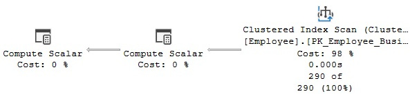
Figure 3.3 – Plan without contradiction detection
However, if I request all employees with more than 300 vacation hours, because of this check constraint, the Query Optimizer must immediately know that no records qualify for the predicate. Run the following query:
SELECT * FROM HumanResources.Employee WHERE VacationHours > 300
As expected, the query will return no records, but this time, it will produce a very different execution plan, as shown in Figure 3.4:
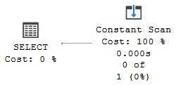
Figure 3.4 – Contradiction detection example
Note that, this time, instead of a Clustered Index Scan, SQL Server is using a Constant Scan operator. The Constant Scan operator introduces one or more constant rows into a query and has virtually no cost. Because there is no need to access the table at all, SQL Server saves resources such as I/O, locks, memory, and CPU, thus making the query execute faster.
Now, let’s see what happens if I disable the check constraint. Run the following statement:
ALTER TABLE HumanResources.Employee NOCHECK CONSTRAINT CK_Employee_VacationHours
This time, running the previous SELECT query once again uses a Clustered Index Scan operator, as the Query Optimizer can no longer use the check constraint to guide its decisions. In other words, it has to scan the entire table, which at this point, has no records that qualify for the VacationHours > 300 predicate.
Don’t forget to enable the constraint again by running the following statement:
ALTER TABLE HumanResources.Employee WITH CHECK CHECK CONSTRAINT
CK_Employee_VacationHours
The second type of contradiction case is when the query itself explicitly contains a contradiction. Take a look at the following query:
SELECT * FROM HumanResources.Employee WHERE VacationHours > 10
AND VacationHours < 5
In this case, no check constraint is involved; both predicates are valid, and each will individually return records. But, they contradict each other when they are run together with an AND operator. As a result, the query returns no records and the plan shows a Constant Scan operator similar to the plan in Figure 3.4.
This may just look like a badly written query that just needs to be fixed. But, remember that some predicates may already be included in, for example, view definitions, and the developer of the query calling the view may be unaware of them. For example, a view may include the VacationHours > 10 predicate, and a developer may call the view using the VacationHours < 5 predicate. Because both predicates contradict each other, a Constant Scan operator will be used again instead. A contradiction may be also difficult to detect by the developer on some complex queries, which we all have in our production environments, even if the contradicting predicates are in the same query.
The following example illustrates the view scenario. Create the following view:
CREATE VIEW VacationHours
AS
SELECT * FROM HumanResources.Employee WHERE VacationHours > 10
Run the following statement using our new view:
SELECT * FROM VacationHours
Nothing out of the ordinary so far. But, the following statement will show again a contradiction detection, even when you cannot see the problem directly in the call to the view. Again, the plan will have a Constant Scan operator as shown in Figure 3.4:
SELECT * FROM VacationHours
WHERE VacationHours < 5
Note
You may try some simple similar queries on your own and not get a contradiction detection behavior. In some cases, a trivial plan may block this behavior.
Now, let’s see the logical trees created during contradiction detection, again using the undocumented 8606 trace flag (enable the 3604 trace flag if needed):
SELECT * FROM HumanResources.Employee WHERE VacationHours > 300
OPTION (RECOMPILE, QUERYTRACEON 8606)
We get the following output (edited to fit the page):
*** Input Tree: ***
LogOp_Project QCOL:[HumanResources].[Employee].BusinessEntityID
LogOp_Select
LogOp_Project
LogOp_Get TBL: HumanResources.Employee TableID=1237579447
TableReferenceID=0 IsRow: COL: IsBaseRow1001
AncOp_PrjList
AncOp_PrjEl QCOL:
[HumanResources].[Employee].OrganizationLevel
ScaOp_UdtFunction EClrFunctionType_UdtMethodGetLevel
IsDet NoDataAccess TI(smallint,Null,ML=2)
ScaOp_Identifier QCOL:
[HumanResources].[Employee].OrganizationNode
ScaOp_Comp x_cmpGt
ScaOp_Identifier QCOL:
[HumanResources].[Employee].VacationHours
ScaOp_Const TI(smallint,ML=2)
AncOp_PrjList
*** Simplified Tree: ***
LogOp_ConstTableGet (0) COL: Chk1000 COL: IsBaseRow1001 QCOL:
[HumanResources].[Employee].BusinessEntityID
The important part to notice is that all the logical operators of the entire input tree are replaced by the simplified tree, consisting only of a LogOp_ConstTableGet operator, which will be later translated into the logical and physical Constant Scan operator we saw previously.
Foreign Key Join elimination
Now, I will show you an example of Foreign Key Join elimination. The following query joins two tables and shows the execution plan in Figure 3.5:
SELECT soh.SalesOrderID, c.AccountNumber
FROM Sales.SalesOrderHeader soh
JOIN Sales.Customer c ON soh.CustomerID = c.CustomerID

Figure 3.5 – Original plan joining two tables
Let’s see what happens if we comment out the AccountNumber column:
SELECT soh.SalesOrderID --, c.AccountNumber
FROM Sales.SalesOrderHeader soh
JOIN Sales.Customer c ON soh.CustomerID = c.CustomerID
If you run the query again, the Customer table and obviously the join operation are eliminated, as can be seen in the execution plan in Figure 3.6:

Figure 3.6 – Foreign Key Join elimination example
There are two reasons for this change in the execution plan. First, because the AccountNumber column is no longer required, no columns are requested from the Customer table. However, it seems like the Customer table has to be included as it is required as part of the equality operation on a join condition. That is, SQL Server needs to make sure that a Customer record exists for each related record in the Individual table.
In reality, this join validation is performed by an existing foreign key constraint, so the Query Optimizer realizes that there is no need to use the Customer table at all. This is the defined foreign key (again, there is no need to run this code):
ALTER TABLE Sales.SalesOrderHeader WITH CHECK ADD CONSTRAINT
FK_SalesOrderHeader_Customer_CustomerID FOREIGN KEY(CustomerID)
REFERENCES Sales.Customer(CustomerID)
As a test, temporarily disable the foreign key by running the following statement:
ALTER TABLE Sales.SalesOrderHeader NOCHECK CONSTRAINT
FK_SalesOrderHeader_Customer_CustomerID
Now, run the previous query with the commented column again. Without the foreign key constraint, SQL Server has no choice but to perform the join operation to make sure that the join condition is executed. As a result, it will use a plan joining both tables again, very similar to the one shown previously in Figure 3.5. Do not forget to re-enable the foreign key by running the following statement:
ALTER TABLE Sales.SalesOrderHeader WITH CHECK CHECK CONSTRAINT
FK_SalesOrderHeader_Customer_CustomerID
Finally, you can also see this behavior on the created logical trees. To see this, use again the undocumented 8606 trace flag, as shown next:
SELECT soh.SalesOrderID --, c.AccountNumber
FROM Sales.SalesOrderHeader soh
JOIN Sales.Customer c ON soh.CustomerID = c.CustomerID
OPTION (RECOMPILE, QUERYTRACEON 8606)
You can see an output similar to this, edited to fit the page:
*** Input Tree: ***
LogOp_Project QCOL: [soh].SalesOrderID
LogOp_Select
LogOp_Join
LogOp_Project
LogOp_Get TBLW: Sales.SalesOrderHeader(alias TBL: soh)
Sales.SalesOrderHeader TableID=1266103551
TableReferenceID=0 IsRow: COL: IsBaseRow1001
AncOp_PrjList
AncOp_PrjEl QCOL: [soh].SalesOrderNumber
ScaOp_Intrinsic isnull
ScaOp_Arithmetic x_aopAdd
…
LogOp_Project
LogOp_Get TBL: Sales.Customer(alias TBL: c)
Sales.Customer TableID=997578592 TableReferenceID=0
IsRow: COL: IsBaseRow1003
AncOp_PrjList
AncOp_PrjEl QCOL: [c].AccountNumber
ScaOp_Intrinsic isnull
ScaOp_Arithmetic x_aopAdd
ScaOp_Const TI(varchar collate
872468488,Var,Trim,ML=2)
ScaOp_Udf dbo.ufnLeadingZeros IsDet
ScaOp_Identifier QCOL: [c].CustomerID
…
*** Simplified Tree: ***
LogOp_Join
LogOp_Get TBL: Sales.SalesOrderHeader(alias TBL: soh)
Sales.SalesOrderHeader TableID=1266103551 TableReferenceID=0
IsRow: COL: IsBaseRow1001
LogOp_Get TBL: Sales.Customer(alias TBL: c) Sales.Customer
TableID=997578592 TableReferenceID=0 IsRow: COL: IsBaseRow1003
ScaOp_Comp x_cmpEq
ScaOp_Identifier QCOL: [c].CustomerID
ScaOp_Identifier QCOL: [soh].CustomerID
*** Join-collapsed Tree: ***
LogOp_Get TBL: Sales.SalesOrderHeader(alias TBL: soh)
Sales.SalesOrderHeader TableID=1266103551 TableReferenceID=0 IsRow: COL:
IsBaseRow1001
In the output, although edited to fit the page, you can see that both the input and the simplified tree still have logical Get operators, or LogOp_Get, for the Sales.SalesOrderHeader and Sales.Customer tables. However, the join-collapsed tree at the end has eliminated one of the tables, showing only Sales.SalesOrderHeader. Notice that the tree was simplified after the original input tree and, after that, the join was eliminated on the join-collapsed tree. We will now check out what trivial plan optimization is.
Trivial plan optimization
The optimization process may be expensive to initialize and run for simple queries that don’t require any cost estimation. To avoid this expensive operation for simple queries, SQL Server uses trivial plan optimization. In short, if there’s only one way, or one obvious best way, to execute the query, depending on the query definition and available metadata, a lot of work can be avoided. For example, the following AdventureWorks2019 query will produce a trivial plan:
SELECT * FROM Sales.SalesOrderDetail
WHERE SalesOrderID = 43659
The execution plan will show whether a trivial plan optimization was performed; the Optimization Level entry in the Properties window of a graphical plan will show TRIVIAL. In the same way, an XML plan will show the StatementOptmLevel attribute as TRIVIAL, as you can see in the next XML fragment:
<StmtSimple StatementCompId=”1” StatementEstRows=”12” StatementId=”1” StatementOptmLevel=”TRIVIAL” StatementSubTreeCost=”0.0032976” StatementText=”SELECT * FROM [Sales].[SalesOrderDetail] WHERE [SalesOrderID]=@1” StatementType=”SELECT” QueryHash=”0x801851E3A6490741” QueryPlanHash=”0x3E34C903A0998272” RetrievedFromCache=”true”>
As I mentioned at the start of this chapter, additional information regarding the optimization process can be shown using the sys.dm_exec_query_optimizer_info DMV, which will produce an output similar to the following for this query:

The output shows that this is in fact a trivial plan optimization, using one table and a maximum DOP of 0, and it also displays the elapsed time and final cost. However, if we slightly change the query to the following, looking up on ProductID rather than SalesOrderID, we now get a full optimization:
SELECT * FROM Sales.SalesOrderDetail
WHERE ProductID = 870
In this case, the Optimization Level or StatementOptLevel property is FULL, which obviously means that the query did not qualify for a trivial plan, and a full optimization was performed instead. Full optimization is used for more complicated queries or queries using more complex features, which will require comparisons of candidate plans’ costs to guide decisions; this will be explained in the next section. In this particular example, because the ProductID = 870 predicate can return zero, one, or more records, different plans may be created depending on cardinality estimations and the available navigation structures. This was not the case in the previous query using the SalesOrderID query, which is part of a unique index, and so it can return only zero or one record.
Finally, you can use an undocumented trace flag, 8757, to disable the trivial plan optimization, which you can use for testing purposes. Let’s try this flag with our previous trivial plan query:
SELECT * FROM Sales.SalesOrderDetail
WHERE SalesOrderID = 43659
OPTION (RECOMPILE, QUERYTRACEON 8757)
If we use the sys.dm_exec_query_optimizer_info DMV again, we can see that now, instead of a trivial plan, we have a hint and the optimization goes to the search 1 phase, which will be explained later in the chapter:

Now that we have learned about trivial plans, we will now check out what joins are and how they help.
Joins
Join ordering is one of the most complex problems in query optimization and one that has been the subject of extensive research since the 1970s. It refers to the process of calculating the optimal join order (that is, the order in which the necessary tables are joined) when executing a query. Because the order of joins is a key factor in controlling the amount of data flowing between each operator in an execution plan, it’s a factor to which the Query Optimizer needs to pay close attention. As suggested earlier, join order is directly related to the size of the search space because the number of possible plans for a query grows very rapidly, depending on the number of tables joined.
A join operation combines records from two tables based on some common information, and the predicate that defines which columns are used to join the tables is called a join predicate. A join works with only two tables at a time, so a query requesting data from n tables must be executed as a sequence of n – 1 joins, although it should be noted that a join does not have to be completed (that is, joined all the required data from both tables) before the next join can be started.
The Query Optimizer needs to make two important decisions regarding joins: the selection of a join order and the choice of a join algorithm. The selection of join algorithms will be covered in Chapter 4, The Execution Engine, so in this section, we will talk about join order. As mentioned, the order in which the tables are joined can greatly impact the cost and performance of a query. Although the results of the query are the same, regardless of the join order, the cost of each different join order can vary dramatically.
As a result of the commutative and associative properties of joins, even simple queries offer many different possible join orders, and this number increases exponentially with the number of tables that need to be joined. The task of the Query Optimizer is to find the optimal sequence of joins between the tables used in the query.
The commutative property of a join between tables A and B states that A JOIN B is logically equivalent to B JOIN A. This defines which table will be accessed first or, said in a different way, which role each table will play in the join. In a Nested Loops Join, for example, the first accessed table is called the outer table and the second one the inner table. In a Hash Join, the first accessed table is the build input, and the second one is the probe input. As we will see in Chapter 4, The Execution Engine, correctly defining which table will be the inner table and which will be the outer table in a Nested Loops Join, or the build input or probe input in a Hash Join, has significant performance and cost implications, and it is a choice made by the Query Optimizer.
The associative property of a join between tables A, B, and C states that (A JOIN B) JOIN C is logically equivalent to A JOIN (B JOIN C). This defines the order in which the tables are joined. For example, (A JOIN B) JOIN C specifies that table A must be joined to table B first, and then the result must be joined to table C. A JOIN (B JOIN C) means that table B must be joined to table C first, and then the result must be joined to table A. Each possible permutation may have different cost and performance results depending, for example, on the size of their temporary results.
As noted earlier, the number of possible join orders in a query increases exponentially with the number of tables joined. In fact, with just a handful of tables, the number of possible join orders could be in the thousands or even millions, although the exact number of possible join orders depends on the overall shape of the query tree. It is impossible for the Query Optimizer to look at all those combinations; it would take far too long. Instead, the SQL Server Query Optimizer uses heuristics to help narrow down the search space.
As mentioned before, queries are represented as trees in the query processor, and the shape of the query tree, as dictated by the nature of the join order, is so important in query optimization that some of these trees have names, such as left-deep, right-deep, and bushy trees. Figure 3.7 shows left-deep and bushy trees for a join of four tables. For example, the left-deep tree could be JOIN( JOIN( JOIN(A, B), C), D), and the bushy tree could be JOIN(JOIN(A, B), JOIN(C, D)):
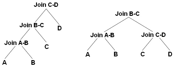
Figure 3.7 – Left-deep and bushy trees
Left-deep trees are also called linear trees or linear processing trees, and you can see how their shapes lead to that description. Bushy trees, on the other hand, can take any arbitrary shape, and so the set of bushy trees includes the sets of both left-deep and right-deep trees.
The number of left-deep trees is calculated as n! (or n factorial), where n is the number of tables in the relation. A factorial is the product of all positive integers less than or equal to n. For example, for a five-table join, the number of possible join orders is 5! = 5 × 4 × 3 × 2 × 1 = 120. The number of possible join orders for a bushy tree is more complicated and can be calculated as (2n – 2)!/(n – 1)!.
The important point to remember here is that the number of possible join orders grows very quickly as the number of tables increases, as highlighted in Table 3.2. For example, in theory, if we had a six-table join, a query optimizer would potentially need to evaluate 30,240 possible join orders. Of course, we should also bear in mind that this is just the number of permutations for the join order. On top of this, a query optimizer also has to evaluate physical join operators and data access methods, as well as optimize other parts of the query, such as aggregations, subqueries, and so on.

Table 3.2 – Possible join orders for left-deep and bushy trees
So, how does the SQL Server Query Optimizer analyze all these possible plan combinations? The answer is it doesn’t. Performing an exhaustive evaluation of all possible combinations for many queries would take too long to be useful, so the Query Optimizer must find a balance between the optimization time and the quality of the resulting plan. As mentioned earlier in the book, the goal of the Query Optimizer is to find a good enough plan as quickly as possible. Rather than exhaustively evaluate every single combination, the Query Optimizer tries to narrow the possibilities down to the most likely candidates, using heuristics (some of which we’ve already touched upon) to guide the process.
Transformation rules
As we’ve seen earlier, the SQL Server Query Optimizer uses transformation rules to explore the search space—that is, to explore the set of possible execution plans for a specific query. Transformation rules are based on relational algebra, taking a relational operator tree and generating equivalent alternatives, in the form of equivalent relational operator trees. At the most fundamental level, a query consists of logical expressions, and applying these transformation rules will generate equivalent logical and physical alternatives, which are stored in memory (in a structure called the Memo) for the entire duration of the optimization process. As explained in this chapter, the Query Optimizer uses up to three optimization stages, and different transformation rules are applied in each stage.
Each transformation rule has a pattern and a substitute. The pattern is the expression to be analyzed and matched, and the substitute is the equivalent expression that is generated as an output. For example, for the commutativity rule, which is explained next, a transformation rule can be defined as follows:
Expr1 join Expr2 – > Expr2 join Expr1
This means that SQL Server will match the Expr1 join Expr2 pattern, as in Individual join Customer, and will produce the equivalent expression, Expr2 join Expr1, or in our case, Customer join Individual. The two expressions are logically equivalent because both return the same results.
Initially, the query tree contains only logical expressions, and transformation rules are applied to these logical expressions to generate either logical or physical expressions. As an example, a logical expression can be the definition of a logical join, whereas a physical expression could be an actual join implementation, such as a Merge Join or a Hash Join. Bear in mind that transformation rules cannot be applied to physical expressions.
The main types of transformation rules include simplification, exploration, and implementation rules. Simplification rules produce simpler logical trees as their outputs and are mostly used during the simplification phase, before the full optimization, as explained previously. Exploration rules, also called logical transformation rules, generate logical equivalent alternatives. Finally, implementation rules, or physical transformation rules, are used to obtain physical alternatives. Both exploration and implementation rules are executed during the full optimization phase.
Examples of exploration rules include the commutativity and associativity rules, which are used in join optimization, and are shown in Figure 3.8:

Figure 3.8 – Commutativity and associativity rules
Commutativity and associativity rules are, respectively, defined as follows:
A join B – > B join A
and
(A join B) join C – > B join (A join C)
The commutativity rule (A join B – > B join A) means that A join B is equivalent to B join A and joining the tables A and B in any order will return the same results. Also, note that applying the commutativity rule twice will generate the original expression again; that is, if you initially apply this transformation to obtain B join A, and then later apply the same transformation, you can obtain A join B again. However, the Query Optimizer can handle this problem to avoid duplicated expressions. In the same way, the associativity rule shows that (A join B) join C is equivalent to B join (A join C) because they also both produce the same results. An example of an implementation rule would be selecting a physical algorithm for a logical join, such as a Merge Join or a Hash Join.
So, the Query Optimizer is using sets of transformation rules to generate and examine possible alternative execution plans. However, it’s important to remember that applying rules does not necessarily reduce the cost of the generated alternatives, and the costing component still needs to estimate their costs. Although both logical and physical alternatives are kept in the Memo structure, only the physical alternatives have their costs determined. It’s important, then, to bear in mind that although these alternatives may be equivalent and return the same results, their physical implementations may have very different costs. The final selection, as is hopefully clear now, will be the best (or, if you like, the cheapest) physical alternative stored in the Memo.
For example, implementing A join B may have different costs depending on whether a Nested Loops Join or a Hash Join is selected. In addition, for the same physical join, implementing the A join B expression may have a different performance from B join A. As explained in Chapter 4, The Execution Engine, the performance of a join is different depending on which table is chosen as the inner or outer table in a Nested Loops Join, or the build and the probe inputs in a Hash Join. If you want to find out why the Query Optimizer might not choose a specific join algorithm, you can test using a hint to force a specific physical join and compare the cost of both the hinted and the original plans.
Those are the foundation principles of transformation rules, and the sys.dm_exec_query_transformation_stats DMV provides information about the existing transformation rules and how they are being used by the Query Optimizer. According to this DMV, SQL Server 2022 CTP 2.0 currently has 439 transformation rules, and more can be added in future updates or versions of the product.
Similar to sys.dm_exec_query_optimizer_info, this DMV contains information regarding the optimizations performed since the time the given SQL Server instance was started and can also be used to get optimization information for a particular query or workload by taking two snapshots of the DMV (before and after optimizing your query) and manually finding the difference between them.
To start looking at this DMV, run the following query:
SELECT * FROM sys.dm_exec_query_transformation_stats
Here is some sample output from my test system using SQL Server 2022, showing the first few records out of 439 (edited to fit the page):
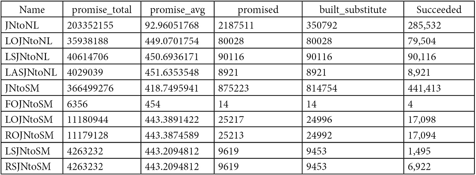
The sys.dm_exec_query_transformation_stats DMV includes what is known as the promise information, which tells the Query Optimizer how useful a given transformation rule might be. The first field in the results output is the name of the rule; for example, the first three rules listed are JNtoNL (Join to Nested Loops Join), LOJNtoNL (Left Outer Join to Nested Loops Join), and JNtoSM (Join to Sort Merge Join), where Sort Merge Join is the academic name of the SQL Server Merge Join operator.
The same issues are shown for the sys.dm_exec_query_optimizer_info DMV regarding collecting data also applies to the sys.dm_exec_query_transformation_stats DMV, so the query shown next can help you to isolate the optimization information for a specific query while avoiding data from related queries as much as possible. The query is based on the succeeded column, which keeps track of the number of times a transformation rule was used and successfully produced a result:
-- optimize these queries now
-- so they do not skew the collected results
GO
SELECT *
INTO before_query_transformation_stats
FROM sys.dm_exec_query_transformation_stats
GO
SELECT *
INTO after_query_transformation_stats
FROM sys.dm_exec_query_transformation_stats
GO
DROP TABLE after_query_transformation_stats
DROP TABLE before_query_transformation_stats
-- real execution starts
GO
SELECT *
INTO before_query_transformation_stats
FROM sys.dm_exec_query_transformation_stats
GO
-- insert your query here
SELECT * FROM Sales.SalesOrderDetail
WHERE SalesOrderID = 43659
-- keep this to force a new optimization
OPTION (RECOMPILE)
GO
SELECT *
INTO after_query_transformation_stats
FROM sys.dm_exec_query_transformation_stats
GO
SELECT a.name, (a.promised - b.promised) as promised
FROM before_query_transformation_stats b
JOIN after_query_transformation_stats a
ON b.name = a.name
WHERE b.succeeded <> a.succeeded
DROP TABLE before_query_transformation_stats
DROP TABLE after_query_transformation_stats
For example, let’s test with a very simple AdventureWorks2019 query, such as the following (which is already included in the previous code):
SELECT * FROM Sales.SalesOrderDetail
WHERE SalesOrderID = 43659
This will show that the following transformation rules are being used:

The plan produced is a trivial plan. Let’s again add the undocumented 8757 trace flag to avoid a trivial plan (just for testing purposes):
SELECT * FROM Sales.SalesOrderDetail
WHERE SalesOrderID = 43659
OPTION (RECOMPILE, QUERYTRACEON 8757)
We would then get the following output:

Let’s now test a more complicated query. Include the following query in the code to explore the transformation rules it uses:
SELECT c.CustomerID, COUNT(*)
FROM Sales.Customer c JOIN Sales.SalesOrderHeader o
ON c.CustomerID = o.CustomerID
GROUP BY c.CustomerID
As shown in the following output, 17 transformation rules were exercised during the optimization process:

The previous query gives us an opportunity to show an interesting transformation rule, GbAggBeforeJoin (or Group By Aggregate Before Join), which is included in the previous list.
The Group By Aggregate Before Join can be used in cases where we have joins and aggregations. A traditional query optimization for this kind of query is to perform the join operation first, followed by the aggregation. An alternative optimization is to push down a group by aggregate before the join. This is represented in Figure 3.9. In other words, if our original logical tree has the shape of the tree on the left in Figure 3.9, after applying GbAggBeforeJoin, we can get the alternate tree on the right, which as expected produces the same query results:

Figure 3.9 – Group By Aggregate Before Join optimization
We can see that GbAggBeforeJoin was applied, as shown on the list of transformation rules earlier, and that the tree on the right was selected, as shown on the final execution plan shown in Figure 3.10:
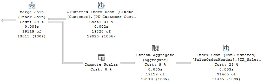
Figure 3.10 – Original execution plan
Here you can see, among other things, that SQL Server is pushing an aggregate below the join (a Stream Aggregate before the Merge Join). The Query Optimizer can push aggregations that significantly reduce cardinality estimation as early in the plan as possible. As mentioned, this is performed by the GbAggBeforeJoin transformation rule (or Group By Aggregate Before Join). This specific transformation rule is used only if certain requirements are met—for example, when the GROUP BY clause includes the joining columns, which is the case in our example.
Now, as I will explain in more detail in Chapter 12, Understanding Query Hints, you may disable some of these transformation rules in order to obtain a specific desired behavior. As a way of experimenting with the effects of these rules, you can also use the undocumented DBCC RULEON and DBCC RULEOFF statements to enable or disable transformation rules, respectively, and thereby, get additional insight into how the Query Optimizer works. However, before you do that, first be warned: because these undocumented statements impact the entire optimization process performed by the Query Optimizer, they should be used only in a test system for experimentation purposes.
To demonstrate the effects of these statements, let’s continue with the same query, copied again here:
SELECT c.CustomerID, COUNT(*)
FROM Sales.Customer c JOIN Sales.SalesOrderHeader o
ON c.CustomerID = o.CustomerID
GROUP BY c.CustomerID
Run the following statement to temporarily disable the use of the GbAggBeforeJoin transformation rule for the current session:
DBCC RULEOFF(‘GbAggBeforeJoin’)
After disabling this transformation rule and running the query again, the new plan, shown in Figure 3.11, will now show the aggregate after the join, which, according to the Query Optimizer, is a more expensive plan than the original. You can verify this by looking at their estimated costs: 0.285331 and 0.312394, for the original plan and the plan with GbAggBeforeJoin disabled, respectively. These costs are not shown in the figures, but you can see them by hovering the mouse over the SELECT icon and examining the Estimated Subtree Cost value, as explained before:
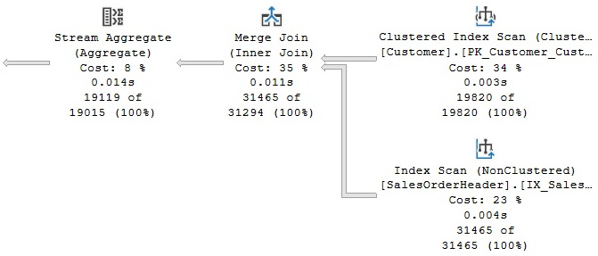
Figure 3.11 – Plan with the GbAggBeforeJoin rule disabled
Note that, for this exercise, an optimization may need to be forced to see the new plan, perhaps using the OPTION (RECOMPILE) hint or one of the methods we’ve discussed to remove the plan from the cache, such as DBCC FREEPROCCACHE.
What’s more, there are a couple of additional undocumented statements to show which transformation rules are enabled and disabled; these are DBCC SHOWONRULES and DBCC SHOWOFFRULES, respectively. By default, DBCC SHOWONRULES will list all the 439 transformation rules listed by the sys.dm_exec_query_transformation_stats DMV. To test it, try running the following code:
DBCC TRACEON (3604)
DBCC SHOWONRULES
We start this exercise by enabling the 3604 trace flag, which, as explained earlier, instructs SQL Server to send the results to the client (in this case, your Management Studio session). After this, the output of DBCC SHOWONRULES (and later, DBCC SHOWOFFRULES), and the DBCC RULEON and DBCC RULEOFF statements will be conveniently available to us. The output is provided next (showing only a few of the possible rules, to preserve space). The previously disabled rule will not be shown in this output:
Rules that are on globally:
JNtoNL
LOJNtoNL
LSJNtoNL
LASJNtoNL
JNtoSM
FOJNtoSM
LOJNtoSM
ROJNtoSM
LSJNtoSM
RSJNtoSM
LASJNtoSM
RASJNtoSM
In the same way, the following code will show the rules that are disabled:
DBCC SHOWOFFRULES
In our case, it will show that only one rule has been disabled:
Rules that are off globally:
GbAggBeforeJoin
DBCC execution completed. If DBCC printed error messages, contact your system administrator.
To continue with our example of the effects of the transformation rules, we can disable the use of a Merge Join by disabling the JNtoSM rule (Join to Sort Merge Join) by running the following code:
DBCC RULEOFF(‘JNtoSM’)
If you have followed the example, this time, DBCC RULEOFF will show some output indicating that the rule is disabled for some specific SPID. For example, the output could be as follows:
DBCC RULEOFF GbAggBeforeJoin SPID 69
This also means that DBCC RULEON and DBCC RULEOFF work at the session level, but even in this case, your exercise may still impact the entire SQL Server instance because your created plans may be kept in the plan cache and potentially reused by other sessions. As a curious note, even when DBCC RULEOFF works at the session level, DBCC SHOWONRULES and DBCC SHOWOFFRULES show messages such as the following:
Rules that are off globally:
These are not exactly true (but after all, they are undocumented statements that users are not supposed to use anyway).
Running the sample query again will give us a new plan, using both a Hash Join and a Hash Aggregate, as shown in Figure 3.12:
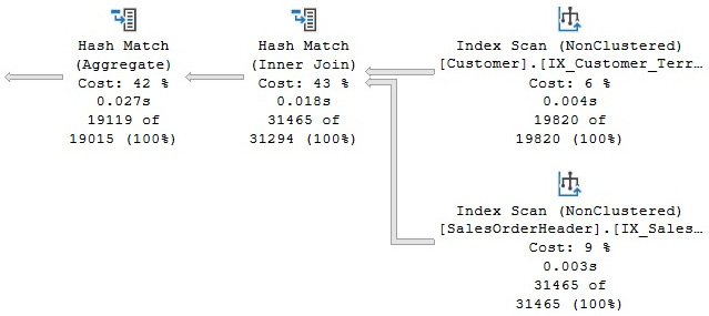
Figure 3.12 – Plan with the JNtoSM rule disabled
So far, we have disabled two optimizations or transformation rules, GbAggBeforeJoin and JNtoSM. This is the reason currently we have the aggregation after the join and we no longer have a Merge Join; instead, the Query Optimizer has selected a Hash Join. Let’s try a couple more changes.
As we will cover in more detail in the next chapter, SQL Server provides two physical algorithms for aggregations, hash, and stream aggregations. Since the current plan in Figure 3.11 is using a Hash Aggregation, let’s disable that choice of algorithm to see what happens. This is performed by disabling the GbAggToHS (Group by Aggregate to Hash) rule, as shown next:
DBCC RULEOFF(‘GbAggToHS’)
After this, we get the plan shown in Figure 3.13:
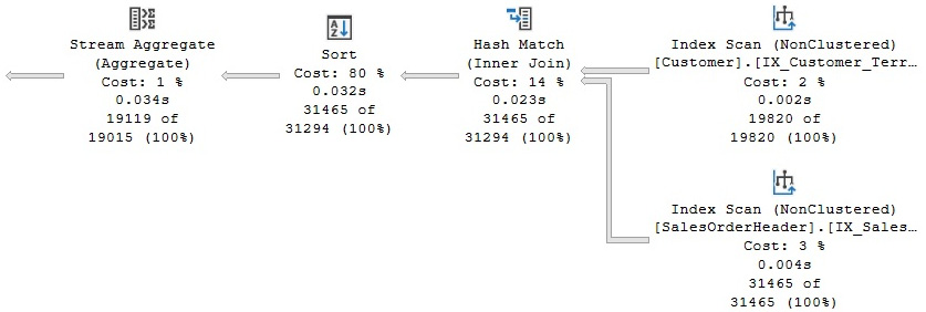
Figure 3.13 – Plan with the GbAggToHS rule disabled
The plan in Figure 3.13 is very similar to the shape of the previous one, but now we have a stream aggregate instead of a hash aggregate. We know that using a stream aggregate is the only choice the Query Optimizer has left. So, what would happen if we also disable stream aggregates? To find out, run the following statement, which disables GbAggToStrm (Group by Aggregate to Stream), and run our test query again:
DBCC RULEOFF(‘GbAggToStrm’)
As expected, the Query Optimizer is not able to get an execution plan and instead gives up returning the following error message:
Msg 8624, Level 16, State 1, Line 186
Internal Query Processor Error: The query processor could not produce a query plan. For more information, contact Customer Support Services.
In Chapter 12,Understanding Query Hints, you will learn how to obtain a similar behavior, disabling specific optimizations or physical operations in your queries, and using hints. Although the statements we covered in this section are undocumented and unsupported, hints are documented and supported but still need to be used very carefully and only when there is no other choice.
Finally, before we finish, don’t forget to reenable the GbAggBeforeJoin and JNtoSM transformation rules by running the following commands:
DBCC RULEON(‘GbAggBeforeJoin’)
DBCC RULEON(‘JNtoSM’)
DBCC RULEON(GbAggToHS’)
DBCC RULEON(GbAggToStrm’)
Then, verify that no transformation rules are still disabled by running the following:
DBCC SHOWOFFRULES
You can also just close your current session since, as mentioned earlier, DBCC RULEON and DBCC RULEOFF work at the session level. You may also want to clear your plan cache (to make sure none of these experiment plans were left in memory) by once again running the following:
DBCC FREEPROCCACHE
A second choice to obtain the same behavior, disabling rules, is to use the also undocumented QUERYRULEOFF query hint, which will disable a rule at the query level. For example, the following code using the QUERYRULEOFF hint will disable the GbAggBeforeJoin rule only for the current optimization:
SELECT c.CustomerID, COUNT(*)
FROM Sales.Customer c JOIN Sales.SalesOrderHeader o
ON c.CustomerID = o.CustomerID
GROUP BY c.CustomerID
OPTION (RECOMPILE, QUERYRULEOFF GbAggBeforeJoin)
You can include more than one rule name while using the QUERYRULEOFF hint, like in the following example, to disable both the GbAggBeforeJoin and JNtoSM rules, as demonstrated before:
SELECT c.CustomerID, COUNT(*)
FROM Sales.Customer c JOIN Sales.SalesOrderHeader o
ON c.CustomerID = o.CustomerID
GROUP BY c.CustomerID
OPTION (RECOMPILE, QUERYRULEOFF GbAggBeforeJoin, QUERYRULEOFF JNtoSM)
Also, the Query Optimizer will obey disabled rules both at the session level and at the query level. Because QUERYRULEOFF is a query hint, this effect lasts only for the optimization of the current query (therefore, no need for a QUERYRULEON hint).
In both cases, DBCC RULEOFF and QUERYRULEOFF, you can be at a point where enough rules have been disabled that the Query Optimizer is not able to produce an execution plan. For example, let’s say you run the following query:
SELECT c.CustomerID, COUNT(*)
FROM Sales.Customer c JOIN Sales.SalesOrderHeader o
ON c.CustomerID = o.CustomerID
GROUP BY c.CustomerID
OPTION (RECOMPILE, QUERYRULEOFF GbAggToStrm, QUERYRULEOFF GbAggToHS)
You would get the following error:
Msg 8622, Level 16, State 1, Line 1
Query processor could not produce a query plan because of the hints defined in this query. Resubmit the query without specifying any hints and without using SET FORCEPLAN
In this particular example, we are disabling both the GbAggToStrm (Group by Aggregate to Stream) and GbAggToHS (Group by Aggregate to Hash) rules. At least one of those rules is required to perform an aggregation; GbAggToStrm would allow me to use a Stream Aggregate and GbAggToHS would allow me to use a Hash Aggregate.
Although the Query Optimizer is, again, not able to produce a valid execution plan, the returned message is very different as this time, the query processor knows the query is using hints. It just simply asks you to resubmit the query without specifying any hints.
Finally, you can also obtain rules information using the undocumented 2373 trace flag. Although it is verbose and provides memory information, it can also be used to find out the transformation rules used during the optimization of a particular query. For example, let’s say you run the following:
SELECT c.CustomerID, COUNT(*)
FROM Sales.Customer c JOIN Sales.SalesOrderHeader o
ON c.CustomerID = o.CustomerID
GROUP BY c.CustomerID
OPTION (RECOMPILE, QUERYTRACEON 2373)
This will show the following output (edited to fit the page):
Memory before rule NormalizeGbAgg: 27
Memory after rule NormalizeGbAgg: 27
Memory before rule IJtoIJSEL: 27
Memory after rule IJtoIJSEL: 28
Memory before rule MatchGet: 28
Memory after rule MatchGet: 28
Memory before rule MatchGet: 28
Memory after rule MatchGet: 28
Memory before rule JoinToIndexOnTheFly: 28
Memory after rule JoinToIndexOnTheFly: 28
Memory before rule JoinCommute: 28
Memory after rule JoinCommute: 28
Memory before rule JoinToIndexOnTheFly: 28
Memory after rule JoinToIndexOnTheFly: 28
Memory before rule GbAggBeforeJoin: 28
Memory after rule GbAggBeforeJoin: 28
Memory before rule GbAggBeforeJoin: 28
Memory after rule GbAggBeforeJoin: 30
Memory before rule IJtoIJSEL: 30
Memory after rule IJtoIJSEL: 30
Memory before rule NormalizeGbAgg: 30
Memory after rule NormalizeGbAgg: 30
Memory before rule GenLGAgg: 30
As covered in this section, applying transformation rules to existing logical and physical expressions will generate new logical and physical alternatives, which are stored in a memory structure called the Memo. Let’s cover the Memo in the next section.
The Memo
The Memo structure was originally defined in The Volcano Optimizer Generator by Goetz Graefe and William McKenna in 1993. In the same way, the SQL Server Query Optimizer is based on the Cascades Framework, which was, in fact, a descendent of the Volcano Optimizer.
The Memo is a search data structure used to store the alternatives generated and analyzed by the Query Optimizer. These alternatives can be logical or physical operators and are organized into groups of equivalent alternatives, such that each alternative in the same group produces the same results. Alternatives in the same group also share the same logical properties, and in the same way that operators can reference other operators on a relational tree, groups can also reference other groups in the Memo structure.
A new Memo structure is created for each optimization. The Query Optimizer first copies the original query tree’s logical expressions into the Memo structure, placing each operator from the query tree in its own group, and then triggers the entire optimization process. During this process, transformation rules are applied to generate all the alternatives, starting with these initial logical expressions.
As the transformation rules produce new alternatives, these are added to their equivalent groups. Transformation rules may also produce a new expression that is not equivalent to any existing group, and that causes a new group to be created. As mentioned before, each alternative in a group is a simple logical or physical expression, such as a join or a scan, and a plan will be built using a combination of these alternatives. The number of these alternatives (and even groups) in a Memo structure can be huge.
Although there is the possibility that different combinations of transformation rules may end up producing the same expressions, as indicated earlier, the Memo structure is designed to avoid both the duplication of these alternatives and redundant optimizations. By doing this, it saves memory and is more efficient because it does not have to search the same plan alternatives more than once.
Although both logical and physical alternatives are kept in the Memo structure, only the physical alternatives are costed. Therefore, at the end of the optimization process, the Memo contains all the alternatives considered by the Query Optimizer, but only one plan is selected, based on the cost of their operations.
Now, I will use some undocumented trace flags to show you how the Memo structure is populated and what its final state is after the optimization process has been completed. We can use the undocumented 8608 trace flag to show the initial content of the Memo structure. Also, notice that a very simple query may not show anything, like in the following example. Remember to enable the 3604 trace flag first:
SELECT ProductID, name FROM Production.Product
OPTION (RECOMPILE, QUERYTRACEON 8608)
The previous query uses a trivial optimization that requires no full optimization and no Memo structure, and therefore, creates a trivial plan. You can force a full optimization by using the undocumented 8757 trace flag and running something like this:
SELECT ProductID, name FROM Production.Product
OPTION (RECOMPILE, QUERYTRACEON 8608, QUERYTRACEON 8757)
In this case, we can see a simple Memo structure like the following:
--- Initial Memo Structure ---
Root Group 0: Card=504 (Max=10000, Min=0)
0 LogOp_Get
Let’s try a simple query that does not qualify for a trivial plan and see its final logical tree using the undocumented 8606 trace flag:
SELECT ProductID, ListPrice FROM Production.Product
WHERE ListPrice > 90
OPTION (RECOMPILE, QUERYTRACEON 8606)
The final tree is as follows:
*** Tree After Project Normalization ***
LogOp_Select
LogOp_Get TBL: Production.Product Production.Product
TableID=1973582069 TableReferenceID=0 IsRow: COL: IsBaseRow1001
ScaOp_Comp x_cmpGt
ScaOp_Identifier QCOL: Production].[Product].ListPrice
ScaOp_Const TI(money,ML=8)
XVAR(money,Not Owned,Value=(10000units)=(900000))
Now, let’s look at the initial Memo structure using the undocumented 8608 trace flag:
SELECT ProductID, ListPrice FROM Production.Product
WHERE ListPrice > 90
OPTION (RECOMPILE, QUERYTRACEON 8608)
We now have something like this:
--- Initial Memo Structure ---
Root Group 4: Card=216 (Max=10000, Min=0)
0 LogOp_Select 0 3
Group 3:
0 ScaOp_Comp 1 2
Group 2:
0 ScaOp_Const
Group 1:
0 ScaOp_Identifier
Group 0: Card=504 (Max=10000, Min=0)
0 LogOp_Get
As you can see, the operators on the final logical tree are copied to and used to initialize the Memo structure, and each operator is placed in its own group. We call group 4 the root group because it is the root operator of the initial plan (that is, the root node of the original query tree).
Finally, we can use the undocumented 8615 trace flag to see the Memo structure at the end of the optimization process:
SELECT ProductID, ListPrice FROM Production.Product
WHERE ListPrice > 90
OPTION (RECOMPILE, QUERYTRACEON 8615)
We would have a Memo structure with the following content:
--- Final Memo Structure ---
Root Group 4: Card=216 (Max=10000, Min=0)
1 PhyOp_Filter 0.2 3.0 Cost(RowGoal 0,ReW 0,ReB 0,Dist 0,Total 0)= 0.0129672
0 LogOp_Select 0 3
Group 3:
0 ScaOp_Comp 1.0 2.0 Cost(RowGoal 0,ReW 0,ReB 0,Dist 0,Total 0)= 3
Group 2:
0 ScaOp_Const Cost(RowGoal 0,ReW 0,ReB 0,Dist 0,Total 0)= 1
Group 1:
0 ScaOp_Identifier Cost(RowGoal 0,ReW 0,ReB 0,Dist 0,Total 0)= 1
Group 0: Card=504 (Max=10000, Min=0)
2 PhyOp_Range 1 ASC Cost(RowGoal 0,ReW 0,ReB 0,Dist 0,Total 0)= 0.0127253
0 LogOp_Get
Now, let’s look at a complete example. Let’s say you run the following query:
SELECT ProductID, COUNT(*)
FROM Sales.SalesOrderDetail
GROUP BY ProductID
OPTION (RECOMPILE, QUERYTRACEON 8608)
This will create the following initial Memo structure:
--- Initial Memo Structure ---
Root Group 18: Card=266 (Max=133449, Min=0)
0 LogOp_GbAgg 13 17
Group 17:
0 AncOp_PrjList 16
Group 16:
0 AncOp_PrjEl 15
Group 15:
0 ScaOp_AggFunc 14
Group 14:
0 ScaOp_Const
Group 13: Card=121317 (Max=133449, Min=0)
0 LogOp_Get
Group 12:
0 AncOp_PrjEl 11
Group 11:
0 ScaOp_Intrinsic 9 10
Group 10:
0 ScaOp_Const
Group 9:
0 ScaOp_Arithmetic 6 8
Group 8:
0 ScaOp_Convert 7
Group 7:
0 ScaOp_Identifier
Group 6:
0 ScaOp_Arithmetic 1 5
Group 5:
0 ScaOp_Arithmetic 2 4
Group 4:
0 ScaOp_Convert 3
Group 3:
0 ScaOp_Identifier
Group 2:
0 ScaOp_Const
Group 1:
0 ScaOp_Convert 0
Group 0:
0 ScaOp_Identifier
Now, run the following query to look at the final Memo structure:
SELECT ProductID, COUNT(*)
FROM Sales.SalesOrderDetail
GROUP BY ProductID
OPTION (RECOMPILE, QUERYTRACEON 8615)
This will show the following output:
--- Final Memo Structure ---
Group 32: Card=266 (Max=133449, Min=0)
0 LogOp_Project 30 31
Group 31:
0 AncOp_PrjList 21
Group 30: Card=266 (Max=133449, Min=0)
0 LogOp_GbAgg 25 29
Group 29:
0 AncOp_PrjList 28
Group 28:
0 AncOp_PrjEl 27
Group 27:
0 ScaOp_AggFunc 26
Group 26:
0 ScaOp_Identifier
Group 25: Card=532 (Max=133449, Min=0)
0 LogOp_GbAgg 13 24
Group 24:
0 AncOp_PrjList 23
…
2 PhyOp_Range 3 ASC Cost(RowGoal 0,ReW 0,ReB 0,Dist 0,Total 0)= 0.338953
0 LogOp_Get
Group 12:
0 AncOp_PrjEl 11
Group 11:
0 ScaOp_Intrinsic 9 10
Group 10:
0 ScaOp_Const
Group 9:
0 ScaOp_Arithmetic 6 8
Group 8:
0 ScaOp_Convert 7
Group 7:
0 ScaOp_Identifier
Group 6:
0 ScaOp_Arithmetic 1 5
Group 5:
0 ScaOp_Arithmetic 2 4
Group 4:
0 ScaOp_Convert 3
Group 3:
0 ScaOp_Identifier
Group 2:
0 ScaOp_Const
Group 1:
0 ScaOp_Convert 0
Group 0:
0 ScaOp_Identifier
The initial Memo structure had 18 groups, and the final went to 32, meaning that 14 new groups were added during the optimization process. As explained earlier, during the optimization process, several transformation rules will be executed that will create new alternatives. If the new alternatives are equivalent to an existing operator, they are placed in the same group as this operator. If not, additional groups will be created. You can also see that group 18 was the root group.
Toward the end of the process, after some implementation rules are applied, equivalent physical operators will be added to the available Memo groups. After the cost for each operator is estimated, the Query Optimizer will look for the cheapest way to assemble a plan using the alternatives available. In this example, the plan selected is shown in Figure 3.14:
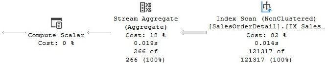
Figure 3.14 – Plan showing operators selected
As we saw earlier, a group by aggregation requires either the GbAggToStrm (Group by Aggregate to Stream) or the GbAggToHS (Group by Aggregate to Hash) transformation rule. In addition, applying any of the techniques explained earlier, you can see that both rules were used in the optimization process; however, only the GbAggToStrm rule was able to create an alternative in group 18, adding the PhyOp_StreamGbAgg physical operator as an equivalent to the original LogOp_GbAgg logical operator. The PhyOp_StreamGbAgg operator is the Stream Aggregate operator that you can see in the final plan, shown in Figure 3.12. Group 18 shows cardinality estimation 266, indicated as Card=266, and an accumulated cost of 0.411876, which you can also verify on the final execution plan. An Index Scan is also shown in the plan, which corresponds to the PhyOp_Range and LogOp_Get operators shown in group 13.
As an additional test, you can see the Memo contents when forcing a Hash Aggregate by running the following query with a hint:
SELECT ProductID, COUNT(*)
FROM Sales.SalesOrderDetail
GROUP BY ProductID
OPTION (RECOMPILE, HASH GROUP, QUERYTRACEON 8615)
Now that we have learned about the Memo, we will explore some optimizer statistics that are handy for gaining insights.
Statistics
To estimate the cost of an execution plan, the query optimizer needs to know, as precisely as possible, the number of records returned by a given query, and to help with this cardinality estimation, SQL Server uses and maintains optimizer statistics. Statistics contain information describing the distribution of values in one or more columns of a table, and will be explained in greater detail in Chapter 6, Understanding Statistics.
As covered in Chapter 1, An Introduction to Query Tuning and Optimization, you can use the OptimizerStatsUsage plan property to identify the statistics used by the Query Optimizer to produce an execution plan. The OptimizerStatsUsage property is available only starting with SQL Server 2017 and SQL Server 2016 SP2. Alternatively, you can use the undocumented 9292 and 9204 trace flags to show similar information about the statistics loaded during the optimization process. Although this method works with all the supported and some older versions of SQL Server, it works only with the legacy cardinality estimation model.
To test these trace flags, run the following exercise. Set the legacy cardinality estimator given as follows:
ALTER DATABASE SCOPED CONFIGURATION
SET LEGACY_CARDINALITY_ESTIMATION = ON
Enable the 3604 trace flag:
DBCC TRACEON(3604)
Run the following query:
SELECT ProductID, name FROM Production.Product
WHERE ProductID = 877
OPTION (RECOMPILE, QUERYTRACEON 9292, QUERYTRACEON 9204)
Once the legacy cardinality estimator is set, the preceding code block produces an output similar to the following:
Stats header loaded: DbName: AdventureWorks2012, ObjName: Production.Product,
IndexId: 1, ColumnName: ProductID, EmptyTable: FALSE
Stats loaded: DbName: AdventureWorks2012, ObjName: Production.Product,
IndexId: 1, ColumnName: ProductID, EmptyTable: FALSE
To better understand how it works, let’s create additional statistics objects. You’ll notice we are creating the same statistics four times.
The 9292 trace flag can be used to display the statistics objects that are considered interesting. Run the following query:
SELECT ProductID, name FROM Production.Product
WHERE ProductID = 877
OPTION (RECOMPILE, QUERYTRACEON 9292)
Here is the output. All the statistics are listed as shown in the following code block:
Stats header loaded: DbName: AdventureWorks2012, ObjName: Production.Product,
IndexId: 1, ColumnName: ProductID, EmptyTable: FALSE
Stats header loaded: DbName: AdventureWorks2012, ObjName: Production.Product,
IndexId: 10, ColumnName: ProductID, EmptyTable: FALSE
Stats header loaded: DbName: AdventureWorks2012, ObjName: Production.Product,
IndexId: 11, ColumnName: ProductID, EmptyTable: FALSE
Stats header loaded: DbName: AdventureWorks2012, ObjName: Production.Product,
IndexId: 12, ColumnName: ProductID, EmptyTable: FALSE
Stats header loaded: DbName: AdventureWorks2012, ObjName: Production.Product,
IndexId: 13, ColumnName: ProductID, EmptyTable: FALSE
The 9204 trace flag can be used to display the statistics objects that were used to produce a cardinality estimate. Test the following code:
SELECT ProductID, name FROM Production.Product
WHERE ProductID = 877
OPTION (RECOMPILE, QUERYTRACEON 9204)
The output is just a single statistics object:
Stats loaded: DbName: AdventureWorks2012, ObjName: Production.Product,
IndexId: 1, ColumnName: ProductID, EmptyTable: FALSE
To clean up, drop the statistics object you’ve just created:
DROP STATISTICS Production.Product.stat1
DROP STATISTICS Production.Product.stat2
DROP STATISTICS Production.Product.stat3
DROP STATISTICS Production.Product.stat4
Do not forget to disable the legacy cardinality estimator:
ALTER DATABASE SCOPED CONFIGURATION
SET LEGACY_CARDINALITY_ESTIMATION = OFF
Finally, as mentioned in Chapter 1, starting with SQL Server 2017 and SQL Server 2016 SP2, you can use the OptimizerStatsUsage XML plan element to identify the statistics used by the Query Optimizer to produce a query plan.
Full optimization
As shown in the processing steps in Figure 3.15, if a query does not qualify for a trivial plan, SQL Server will run the cost-based optimization process, which uses transformation rules to generate alternative plans, stores these alternatives in the Memo structure, and uses cost estimation to select the best plan. This optimization process can be executed in up to three stages or phases, with different transformation rules being applied at each stage.
Because some queries may have a huge number of possible query plans, it’s sometimes not feasible to explore their entire search space—query optimization would take too long. So, in addition to applying transformation rules, several heuristics are used by the Query Optimizer to control the search strategy and to limit the number of alternatives generated to quickly find a good plan. The Query Optimizer needs to balance the optimization time and the quality of the selected plan. For example, as explained earlier, optimizing join orders can create a huge number of possible alternatives. So, a heuristic used by SQL Server creates an initial set of join orders based on their selectivity, as shown later in this section.
In addition, as introduced in Chapter 1, An Introduction to Query Tuning and Optimization, the optimization process can immediately finish if a good enough plan is found, relative to the Query Optimizer’s internal thresholds, at the end of any of the three optimization phases (explained next). However, if at the end of any given phase the best plan is still very expensive, the Query Optimizer will run the next phase, which will run an additional set of (usually more complex) transformation rules. These phases are called search 0, search 1, and search 2 on the sys.dm_exec_query_optimizer_info DMV and are shown in Figure 3.15:

Figure 3.15 – The optimization process
Let’s examine those three search phases in more detail.
Search 0
Similar to the concept of the trivial plan, the first phase, search 0, will aim to find a plan as quickly as possible without trying sophisticated transformations. Search 0, called the transaction processing phase, is ideal for the small queries typically found on transaction-processing systems and it is used for queries with at least three tables. Before the full optimization process is started, the Query Optimizer generates the initial set of join orders based on heuristics. These heuristics begin by first joining the smallest tables or the tables that achieve the largest filtering based on their selectivity. Those are the only join orders considered on search 0. At the end of this phase, the Query Optimizer compares the cost of the best-generated plan to an internal cost threshold. If the best plan is cheap enough compared to this threshold, the plan is selected and the query optimization process stops. If the plan is still very expensive, SQL Server will run the next phase.
Search 1
The next phase, search 1 (also called Quick Plan), uses additional transformation rules, and limited join reordering, and is appropriate for more complex queries. At the end of this phase, SQL Server compares the cost of the cheapest plan to a second internal cost threshold; if the best plan is cheap enough, it is selected. If the query is still expensive and the system can run parallel queries, this phase is executed again to find a good parallel plan, but no plan is selected for execution at this point. At the end of this phase, the costs of the best serial and parallel plans are compared, and the cheapest one is used in the following phase, search 2, which we’ll come to in just a moment.
As an example, the following query does not qualify for search 0 and will go directly to search 1:
SELECT * FROM Sales.SalesOrderDetail
WHERE ProductID = 870
Using the sys.dm_exec_query_optimizer_info DMV, as explained earlier in this chapter, you can display its optimization information seen next, which shows that only the search 1 phase was executed:

The sys.dm_exec_query_optimizer_info DMV includes a counter named gain stage 0 to stage 1, which shows the number of times search 1 was executed after search 0, and includes the average decrease in cost from one stage to the other, as defined by the following formula:
(MinimumPlanCost(search 0) – MinimumPlanCost(search 1)) / MinimumPlanCost(search 0)
For example, run the following query:
SELECT soh.SalesOrderID, sod.SalesOrderDetailID, SalesReasonID
FROM Sales.SalesOrderHeader soh
JOIN Sales.SalesOrderDetail sod
ON soh.SalesOrderID = soh.SalesOrderID
JOIN Sales.SalesOrderHeaderSalesReason sohsr
ON sohsr.SalesOrderID = soh.SalesOrderID
WHERE soh.SalesOrderID = 43697
This will provide the optimization information shown next:

The output shows that the optimization process went through both the search 0 and search 1 stage and that a plan was found on the latter. It also shows a cost improvement of 5 percent by going from the search 0 stage to the search 1 stage.
Search 2
The last phase, search 2, is called full optimization and is used for queries ranging from complex to very complex. A larger set of the potential transformation rules, parallel operators, and other advanced optimization strategies are considered in this phase. Because this is the last phase, an execution plan must be found here (perhaps with the exception of the timeout event, as explained later).
The sys.dm_exec_query_optimizer_info DMV includes another useful counter, named gain stage 1 to stage 2, to show the number of times search 2 was executed after search 1, together with the average decrease in cost from one stage to the other, as defined by the following formula:
(MinimumPlanCost(search 1) – MinimumPlanCost(search 2)) / MinimumPlanCost(search 1)
We could also use the undocumented 8675 and 2372 trace flags to get additional information about these optimization phases. For example, run the following query using the 8675 trace flag:
SELECT DISTINCT pp.LastName, pp.FirstName
FROM Person.Person pp JOIN HumanResources.Employee e
ON e.BusinessEntityID = pp.BusinessEntityID
JOIN Sales.SalesOrderHeader soh
ON pp.BusinessEntityID = soh.SalesPersonID
JOIN Sales.SalesOrderDetail sod
ON soh.SalesOrderID = soh.SalesOrderID
JOIN Production.Product p
ON sod.ProductID = p.ProductID
WHERE ProductNumber = ‘BK-M18B-44’
OPTION (RECOMPILE, QUERYTRACEON 8675)
It will create the optimization information shown next:
End of simplification, time: 0.003 net: 0.003 total: 0.003 net: 0.003
end exploration, tasks: 149 no total cost time: 0.005 net: 0.005 total: 0.009
end search(0), cost: 13.884 tasks: 332 time: 0.002 net: 0.002 total: 0.011
end exploration, tasks: 926 Cost = 13.884 time: 0.01 net: 0.01 total: 0.021
end search(1), cost: 3.46578 tasks: 1906 time: 0.009 net: 0.009 total: 0.031
end exploration, tasks: 3301 Cost = 3.46578 time: 0.008 net: 0.008 total: 0.04
*** Optimizer time out abort at task 4248 ***
end search(2), cost: 0.832242 tasks: 4248 time: 0.013 net: 0.013 total: 0.053
*** Optimizer time out abort at task 4248 ***
End of post optimization rewrite, time: 0 net: 0 total: 0.053 net: 0.053
End of query plan compilation, time: 0 net: 0 total: 0.054 net: 0.054
The optimization information shows that this query went throughout all the three stages of optimization and had optimization time out on search 2. The optimization timeout concept was briefly introduced in Chapter 1, An Introduction to Query Tuning and Optimization, and will be explained next.
Running the same query with the 2372 trace flag will show the following output, in which the search 0, 1, and 2 phases are named stage TP, QuickPlan, and Full, respectively:
Memory before NNFConvert: 25
Memory after NNFConvert: 25
Memory before project removal: 27
Memory after project removal: 29
Memory before simplification: 29
Memory after simplification: 58
Memory before heuristic join reordering: 58
Memory after heuristic join reordering: 65
Memory before project normalization: 65
Memory after project normalization: 65
Memory before stage TP: 68
Memory after stage TP: 84
Memory before stage QuickPlan: 84
Memory after stage QuickPlan: 126
Memory before stage Full: 126
Memory after stage Full: 172
Memory before copy out: 172
Memory after copy out: 173
As we’ve touched upon previously, the Query Optimizer has to find the best plan possible within the shortest amount of time. More to the point, it must eventually return a plan, even if that plan is not as efficient as it would like. To that end, the optimization process also includes the concept of an optimization cost budget. When this budget is exceeded, the search for the optimal plan is terminated, and the Query Optimizer will show an optimization timeout. This timeout is not a fixed amount of time but is instead calculated based on the number of transformations applied together with the elapsed time.
When a timeout is found, the Query Optimizer stops the optimization process and returns the least expensive plan it has found so far. The best plan found so far could be a plan found during the current optimization stage, but most likely, it would be the best plan found in the previous stage. This means that a timeout most likely will happen in the search 1 and search 2 stages. This timeout event is shown in the properties of a graphical plan as Reason For Early Termination Of Statement Optimization or in an XML plan as StatementOptmEarlyAbortReason. This event is also shown as the timeout counter on the sys.dm_exec_query_optimizer_info DMV. An example is shown in the following XML fragment, obtained by running the previous query in this section:
<StmtSimple StatementCompId=”1”
StatementEstRows=”1”
StatementId=”1”
StatementOptmLevel=”FULL”
StatementOptmEarlyAbortReason=”TimeOut”
CardinalityEstimationModelVersion=”140”
…
>
Finally, at the end of the optimization process, the chosen plan will be sent to the execution engine to be run, and the results will be sent back to the client.
Summary
This chapter showed how the Query Optimizer works, explaining how your query goes from a SQL statement submitted to SQL Server, all the way to the selected execution plan, including operations such as parsing, binding, simplification, trivial plan, and the full optimization stages. Important concepts that are part of the Query Optimizer architecture, such as transformation rules and the Memo structure, were also introduced.
The Query Optimizer generates a solution space and selects the best possible execution plan from it based on the plan cost. Transformation rules are used to generate these alternatives, which are stored in a memory structure called the Memo. Instead of exploring the search space exhaustively, heuristics are introduced to limit the number of possible solutions. Finally, the alternatives stored in the Memo are costed, and the best solution is returned for execution.
This chapter also showed that understanding how the Query Optimizer works can give you a great background to troubleshoot, optimize, and better tune your queries. But, you still need to learn more about the most-used query operators employed on the plans created by the Query Optimizer. We will cover that topic in the next chapter.
|
Updated |
Rows Above |
Rows Below |
Inserts Since Last Update |
Deletes Since Last Update |
Leading column Type |
|
Jun 7 2022 |
32 |
0 |
32 |
0 |
Ascending |
|
Jun 7 2022 |
27 |
0 |
27 |
0 |
NULL |
|
Jun 7 2022 |
30 |
0 |
30 |
0 |
NULL |
|
Jun 7 2022 |
NULL |
NULL |
NULL |
NULL |
NULL |
|
Updated |
Rows Above |
Rows Below |
Inserts Since Last Update |
Deletes Since Last Update |
Leading column Type |
|
Jun 7 2022 |
27 |
0 |
27 |
0 |
Unknown |
|
Jun 7 2022 |
30 |
0 |
30 |
0 |
NULL |
|
Jun 7 2022 |
NULL |
NULL |
NULL |
NULL |
NULL |