Chapter 11: An Introduction to Data Warehouses

Usually, when we read about high-performing applications in a SQL Server book or article, we assume they are only talking about transactional applications and, of course, online transaction processing (OLTP) databases. Although we have not mentioned data warehouses so far in this book, most of the content applies to both OLTP databases and data warehouse databases. The SQL Server query optimizer can automatically identify and optimize data warehouse queries without any required configuration, so the concepts explained in this book regarding query optimization, query operators, indexes, statistics, and more apply to data warehouses, too.

In this chapter, we will cover topics that are only specific to data warehouses. Additionally, describing what a data warehouse is provides us with the opportunity to define OLTP systems and what the differences between both are. We will describe how the query optimizer identifies data warehouse queries and cover some of the data warehouse optimizations introduced in the last few versions of SQL Server.

Bitmap filtering, an optimization used in star join queries and introduced with SQL Server 2008, can be used to filter out rows from a fact table very early during query processing, thus significantly improving the performance of data warehouse queries. Bitmap filtering is based on Bloom filters – a space-efficient probabilistic data structure originally conceived by Burton Howard Bloom in 1970.

Columnstore indexes, a feature introduced with SQL Server 2012, introduce us to two new paradigms: columnar-based storage and new batch-processing algorithms. Although columnstore indexes had some limitations when they were originally released—mostly, the fact that the indexes were not updatable and only nonclustered indexes could be created—these limitations have been addressed in later releases. The star join query optimization is an Enterprise Edition-only feature. Additionally, the xVelocity memory-optimized columnstore indexes started as an Enterprise Edition-only feature, but as of SQL Server 2016 Service Pack 1, are available on all the editions of the product.

In this chapter, we will cover the following topics:

• Data warehouses
• Star join query optimization
• Columnstore indexes

Data warehouses

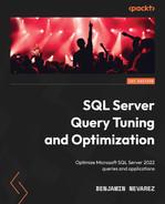
Usually, the information within an organization is kept in one of two forms—in an operational system or in an analytical system—both of which have very different purposes. Although the purpose of an operational system, which is also known as an OLTP system, is to support the execution of a business process, the purpose of an analytic system or data warehouse is to help with the measurement of a business process and business decision-making. OLTP systems are based on small, high-performance transactions consisting of INSERT, DELETE, UPDATE, and SELECT statements, while a data warehouse is based on large and complex queries of aggregated data. The degree of normalization is another main difference between these systems: while an OLTP system will usually be in the third normal form, a data warehouse will use a denormalized dimensional model called a star schema. The third normal form used by OLTP systems helps with data integrity and data redundancy problems because update operations only need to be updated in one place. A data warehouse dimensional model is more appropriate for ad hoc complex queries.

We can see a summary of the differences between operational and analytic systems, as detailed in Table 11.1:

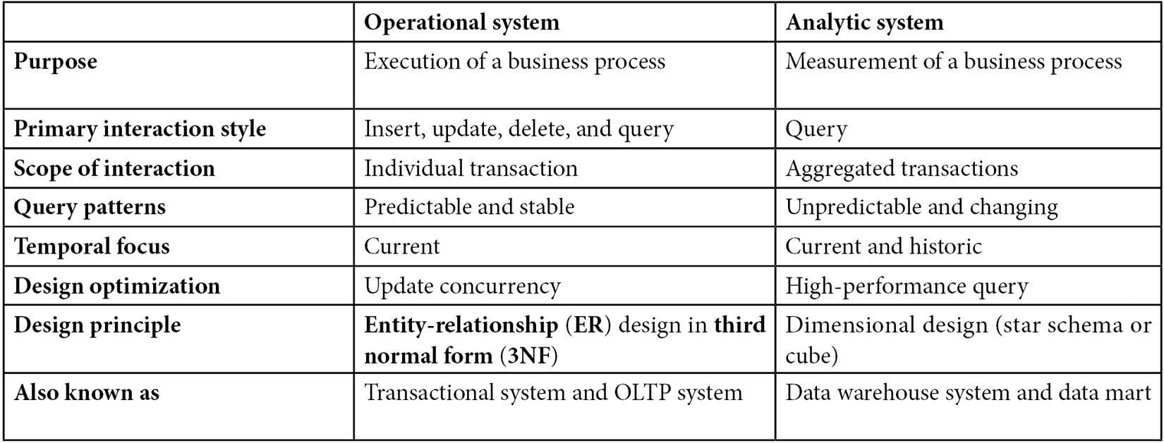
Table 11.1 – Comparing operational and analytic systems

A dimensional design, when implemented in a relational database such as SQL Server, is called a star schema. Data warehouses using a star schema use fact and dimension tables, where fact tables contain the business’s facts or numerical measures, which can participate in calculations, and dimension tables contain the attributes or descriptions of the facts. Not everything that is numeric is a fact, which can be the case with numeric data such as phone numbers, age, and size information. Sometimes, additional normalization is performed within dimension tables in a star schema, which is called a snowflake schema.

SQL Server includes a sample data warehouse database, AdventureWorksDW2019, which follows a snowflake design and will be used in the examples for this chapter. Figure 11.1 shows a diagram with some of the fact and dimension tables of AdventureWorksDW2019:

Figure 11.1 – Fact and dimension tables in AdventureWorksDW2019

Usually, fact tables are very large and can store millions or billions of rows, compared to dimension tables, which are significantly smaller. The size of data warehouse databases tends to range from hundreds of gigabytes to terabytes. Facts are stored as columns in a fact table, while related dimensions are stored as columns in dimension tables. Usually, fact tables have foreign keys to link them to the primary keys of the dimension tables. When used in queries, facts are usually aggregated or summarized, whereas dimensions are used as filters or query predicates. Additionally, a dimension table has a surrogate key, usually an integer, which is also the primary key of the table. For example, in AdventureWorksDW2019, the DimCustomer table has CustomerKey, which is also its primary key, and it is defined as an identity.

Note

More details about data warehousing and dimensional designs can be found in The Data Warehouse Toolkit (Wiley, 2013), by Ralph Kimball and Margy Ross, and Star Schema: The Complete Reference, by Christopher Adamson.

The world of data is rapidly evolving, and new trends such as increasing data volumes and new sources and types of data, along with the new requirement of support for near real-time processing, are changing the traditional data warehouse. In some cases, new approaches are being proposed in response to these trends.

Although SQL Server Enterprise Edition allows you to handle large data warehouses and contains the star join query optimizations and xVelocity memory-optimized columnstore indexes covered in this chapter, SQL Server is also available as an appliance that can allow companies to handle databases of up to 6 petabytes (PB) of data storage. Built on a Multiple Parallel Processing (MPP) architecture with preinstalled software, SQL Server Parallel Data Warehouse provides a highly scalable architecture to help with these large data warehouses. In April 2014, Microsoft announced the Analytics Platform System (APS), which is an appliance solution with hardware and software components that include SQL Server Parallel Data Warehouse and Microsoft’s Hadoop distribution, HDInsight, which is based on the Hortonworks Data Platform.

Finally, in SQL Server 2022, Azure Synapse Link for SQL will allow you to get near real-time analytics over operational data. This new feature will allow you to run business intelligence, analytics, and machine learning scenarios on SQL Server 2022 operational data with minimum impact on source databases. Currently, Azure Synapse Link for SQL is in preview, and you can get more information about it by looking at https://docs.microsoft.com/en-us/azure/synapse-analytics/synapse-link/sql-synapse-link-overview.

Now that we have had a brief introduction to data warehouses, let’s dive into a key feature in SQL Server for it.

Star join query optimization

Queries that join a fact table to dimension tables are called star join queries, and SQL Server includes special optimizations for this kind of query. A typical star join query joins a fact table with one or more dimension tables, groups by some columns of the dimension tables, and aggregates on one or more columns of the fact table. In addition to the filters applied when the tables are joined, other filters can be applied to the fact and dimension tables. Here is an example of a typical star join query in AdventureWorksDW2019 showing all the characteristics that were just mentioned:

SELECT TOP 10 p.ModelName, p.EnglishDescription,

SUM(f.SalesAmount) AS SalesAmount

FROM FactResellerSales f JOIN DimProduct p

ON f.ProductKey = p.ProductKey

JOIN DimEmployee e

ON f.EmployeeKey = e.EmployeeKey

WHERE f.OrderDateKey >= 20030601

AND e.SalesTerritoryKey = 1

GROUP BY p.ModelName, p.EnglishDescription

ORDER BY SUM(f.SalesAmount) DESC

Sometimes, because data warehouse implementations do not completely specify the relationships between fact and dimension tables and do not explicitly define foreign key constraints in order to avoid the overhead of constraint enforcement during updates, SQL Server uses heuristics to automatically detect star join queries and can reliably identify fact and dimension tables. One such heuristic is to consider the largest table of the star join query as the fact table, which must have a specified minimum size, too. In addition, to qualify for a star join query, the join conditions must be inner joins and all the join predicates must be single-column equality predicates. It is worth noting that even in cases where these heuristics do not work correctly and one dimension table is incorrectly chosen as a fact table, a valid plan returning correct data is still selected, although it might not be an efficient one.

Based on the selectivity of a fact table, SQL Server can define three different approaches to optimize star join queries. For highly selective queries, which could return up to 10 percent of the rows of the table, SQL Server might produce a plan with Nested Loops Joins, Index Seeks, and bookmark lookups. For medium-selectivity queries, processing anywhere from 10 percent to 75 percent of the rows in a table, the query optimizer might recommend hash joins with bitmap filters, in combination with fact table scans or fact table range scans. Finally, for the least selective of the queries, returning more than 75 percent of the rows of the table, SQL Server might recommend regular hash joins with fact table scans. The choice of these operators and plans is not surprising for the most and least selective queries because this is their standard behavior, as explained in Chapter 4, The Execution Engine. However, what is new is the choice of hash joins and bitmap filtering for medium-selectivity queries; therefore, we will be looking at those optimizations next. But first, let’s introduce bitmap filters.

Although bitmap filters are used on the star join optimization covered in this section, they have been used in SQL Server since version 7.0. Also, they might appear on other plans, an example of which was shown at the end of the Parallelism section in Chapter 4, The Execution Engine. Bitmap filters are based on Bloom filters, a space-efficient probabilistic data structure originally conceived by Burton Bloom in 1970. Bitmap filters are used in parallel plans, and they greatly improve the performance of these plans by performing a semi-join reduction early in the query before rows are passed through the parallelism operator. Although it is more common to see bitmap filters with hash joins, they could be used by Merge Join operators, too.

As explained in Chapter 4, The Execution Engine, a hash join operation has two phases: build and probe. In the build phase, all the join keys of the build or outer table are hashed into a hash table. A bitmap is created as a byproduct of this operation, and the bits in the array are set to correspond with hash values that contain at least one row. The bitmap is later examined when the probe or inner table is being read. If the bit is not set, the row cannot have a match in the outer table and is discarded.

Bitmap filters are used in star join queries to filter out rows from the fact table very early during query processing. This optimization was introduced in SQL Server 2008, and your existing queries can automatically benefit from it without any changes. This optimization is referred to as optimized bitmap filtering in order to differentiate it from the standard bitmap filtering that was available in previous versions of SQL Server. Although standard bitmap filtering can be used in plans with hash joins and Merge Join operations, as indicated earlier, optimized bitmap filtering is only allowed on plans with hash joins. The Opt_ prefix in the name of a bitmap operator indicates an optimized bitmap filter is being used.

To filter out rows from the fact table, SQL Server builds the hash tables on the “build input” side of the hash join (which, in our case, is a dimension table), constructing a bitmap filter that is an array of bits, which is later used to filter out rows from the fact table that do not qualify for the hash joins. There might be some false positives, meaning that some of the rows might not participate in the join, but there are no false negatives. SQL Server then passes the bitmaps to the appropriate operators to help remove any nonqualifying rows from the fact table early in the query plan.

Multiple filters can be applied to a single operator, and optimized bitmap filters can be applied to exchange operators, such as Distribute Streams and Repartition Streams operators, and filter operators. An additional optimization while using bitmap filters is the in-row optimization, which allows you to eliminate rows even earlier during query processing. When the bitmap filter is based on not-nullable big or bigint columns, the bitmap filter could be applied directly to the table operation. An example of this is shown next.

For this example, let’s run the following query:

SELECT TOP 10 p.ModelName, p.EnglishDescription,

SUM(f.SalesAmount) AS SalesAmount

FROM FactResellerSales f JOIN DimProduct p

ON f.ProductKey = p.ProductKey

JOIN DimEmployee e

ON f.EmployeeKey = e.EmployeeKey

WHERE f.OrderDateKey >= 20030601

AND e.SalesTerritoryKey = 1

GROUP BY p.ModelName, p.EnglishDescription

ORDER BY SUM(f.SalesAmount) DESC

With the current size of AdventureWorksDW2019, this query is not even expensive enough to generate a parallel plan because its cost is only 1.98374. Although we can do a little trick to simulate more records on this database, we encourage you to test this or similar queries in your data warehouse development or test environment.

To simulate a larger table with 100,000 rows and 10,000 pages, run the following statement:

UPDATE STATISTICS dbo.FactResellerSales WITH ROWCOUNT = 100000, PAGECOUNT = 10000

Note

The undocumented ROWCOUNT and PAGECOUNT choices of the UPDATE STATISTICS statement were introduced in Chapter 6, Understanding Statistics. As such, they should not be used in a production environment. They will only be used in this exercise to simulate a larger table.

Clean the plan cache by running a statement such as the following:

DBCC FREEPROCCACHE

Then, run the previous star join query again. This time, we get a more expensive query and a different plan, which is partially shown in Figure 11.2:

Figure 11.2 – A plan with an optimized bitmap filter

As explained earlier, you can see that a bitmap filter was created on the build input of the hash join, which, in this case, reads data from the DimEmployee dimension table. Looking at Defined Values in the bitmap operator’s Properties window, you can see that, in this case, the name of the bitmap filter shows the Opt_Bitmap1006 value. Now, look at the properties of the Clustered Index Scan operator, which are shown in Figure 11.3. Here, you can see that the previously created bitmap filter, Opt_Bitmap1006, is used in the Predicate section to filter out rows from the FactResellerSales fact table. Also, notice the IN ROW parameter, which shows that in-row optimization was also used, thus filtering out rows from the plan as early as possible (in this case, from the Clustered Index Scan operation):

[AdventureWorksDW2019].[dbo].[FactResellerSales].[OrderDateKey] as [f]. [OrderDateKey]>=(20030601) AND PROBE([Opt_Bitmap1006], [AdventureWorksDW2019].[dbo].[FactResellerSales].[EmployeeKey] as [f]. [EmployeeKey],N’[IN ROW]’) 

Finally, run the following statement to correct the page and row count we just changed in the FactResellerSales table:

DBCC UPDATEUSAGE (AdventureWorksDW2019, ‘dbo.FactResellerSales’) WITH COUNT_ROWS

Now that we have learned about star query optimization, we will explore another useful feature for data warehouses: columnstore indexes.

Columnstore indexes

When SQL Server 2012 was originally released, one of the main new features was columnstore indexes. By using a new column-based storage approach and new query-processing algorithms, memory-optimized columnstore indexes were designed to improve the performance of data warehouse queries by several orders of magnitude. Although the inability to update data was the biggest drawback when this feature was originally released back in 2012, this limitation was addressed in the following release. From SQL Server 2014 onward, it has the ability to directly update its data and even create a columnstore clustered index on it. The fact that columnstore indexes were originally limited to only nonclustered indexes was also considered a limitation because it required duplicated data on an already very large object such as a fact table. That is, all the indexed columns would be both on the base table and in the columnstore index.

As mentioned at the beginning of this chapter, in an OLTP system, transactions usually access one row or a few rows, whereas typical data warehouse star join queries access a large number of rows. In addition, an OLTP transaction usually accesses all of the columns in the row, which is opposite to a star join query, where only a few columns are required. This data access pattern showed that a columnar approach could benefit data warehouse workloads.

The traditional storage approach used by SQL Server is to store rows on data pages, which we call a “rowstore.” Rowstores in SQL Server include heaps and B-tree structures, such as standard clustered and nonclustered indexes. Column-oriented storage such as the one used by columnstore indexes dedicates entire database pages to store data from a single column. Rowstores and columnstores are compared in Figure 11.3, where a rowstore contains pages with rows, with each row containing all its columns, and a columnstore contains pages with data for only one column, labeled C1, C2, and so on. Because the data is stored in columns, one question that is frequently asked is how a row is retrieved from this columnar storage. It is the position of the value in the column that indicates to which row this data belongs. For example, the first value on each page (C1, C2, and so on), as shown in Figure 11.3, belongs to the first row, the second value on each page belongs to the second row, and so on:

Figure 11.3 – Rowstore and columnstore data layout comparison

Column-oriented storage is not new and has been used before by some other database vendors. Columnstore indexes are based on Microsoft xVelocity technology, formerly known as VertiPaq, which is also used in SQL Server Analysis Services (SSAS), Power Pivot for Excel, and SharePoint. Similar to the in-memory OLTP feature, as covered in Chapter 7, columnstore indexes are also an in-memory technology.

As mentioned earlier, columnstore indexes dedicate entire database pages to store data from a single column. Also, columnstore indexes are divided into segments, which consist of multiple pages, and each segment is stored in SQL Server as a separate BLOB. As indicated earlier, as of SQL Server 2014, it is now possible to define a columnstore index as a clustered index, which is a great benefit because there is no need for duplicated data. For example, in SQL Server 2012, a nonclustered columnstore index had to be created on a heap or regular clustered index, thus duplicating the data on an already large fact table.

Performance benefits

Columnstore indexes provide increased performance benefits based on the following:

• Reduced I/O: Because rowstore pages contain all the columns in a row, in a data warehouse without columnstore indexes, SQL Server has to read all of the columns, including the columns that are not required by the query. Typical star join queries use only between 10 percent and 15 percent of the columns in a fact table. Based on this, using a columnstore to only read those columns can represent savings of between 85 percent and 90 percent in disk I/O, compared to a rowstore.
• Batch mode processing: New query-processing algorithms are designed to process data in batches and are very efficient at handling large amounts of data. Batch mode processing is explained in more detail in the next section.
• Compression: Because data from the same column is stored contiguously on the same pages, usually, they will have similar or repeated values that can often be compressed more effectively. Compression can improve performance because fewer disk I/O operations are needed to read compressed data and more data can fit into memory. Columnstore compression is not the same as the row and page compression that has been available since SQL Server 2008 and, instead, uses the VertiPaq compression algorithms. However, one difference is that, in columnstore indexes, column data is automatically compressed and compression cannot be disabled, whereas row and page compression in rowstores is optional and has to be explicitly configured.
• Segment elimination: As indicated earlier, columnstore indexes are divided into segments, and SQL Server keeps the minimum and maximum values for each column segment in the sys.column_store_segments catalog view. This information can be used by SQL Server to compare against query filter conditions to identify whether a segment can contain the requested data, thus avoiding reading segments that are not needed and saving both I/O and CPU resources.

Because data warehouse queries using columnstore indexes can now be executed, in many cases, several orders of magnitude faster than with tables defined as rowstore, they can provide other benefits too, such as reducing or eliminating the need to rely on prebuilt aggregates such as OLAP cubes, indexed views, and summary tables. The only action required to benefit from these performance improvements is to define the columnstore indexes in your fact tables. There is no need to change your queries or use any specific syntax; the query optimizer will automatically consider the columnstore index—although, as always, whether or not it is used in a plan will be a cost-based decision. Additionally, columnstore indexes provide more flexibility to changes than building these prebuilt aggregates. If a query changes, the columnstore index will still be useful, and the query optimizer will automatically react to those query changes, whereas the prebuilt aggregate might no longer be able to support the new query or might require changes to accommodate it.

Batch mode processing

As covered in Chapter 1, An Introduction to Query Tuning and Optimization, when we talked about the traditional query-processing mode in SQL Server, you saw that operators request rows from other operators one row at a time—for example, using the GetRow() method. This row processing mode works fine for transactional OLTP workloads where queries are expected to produce only a few rows. However, for data warehouse queries, which process large amounts of rows to aggregate data, this one-row-at-a-time processing mode could become very expensive.

With columnstore indexes, SQL Server is not only providing columnar-based storage but is also introducing a query-processing mode that processes a large number of records, one batch at a time. A batch is stored as a vector in a separate area of memory and, typically, represents about 1,000 rows of data. This also means that query operators can now run in either row mode or batch mode. Starting with SQL Server 2012, only a few operators can run in either batch mode or row mode, and those operators include Columnstore Index Scan, Hash Aggregate, Hash Join, Project, and Filter. Another operator, Batch Hash Table Build, works only in batch mode; it is used to build a batch hash table for the memory-optimized columnstore index in a hash join. In SQL Server 2014, the number of batch mode operators has been expanded, and existing operators, especially the Hash Join operator, have been improved.

It is worth noting that a plan with both row- and batch-processing operators might have some performance degradation, as communication between row mode and batch mode operators is more expensive than the communication between operators running in the same mode. As a result, each transition has an associated cost that the query optimizer uses to minimize the number of these transitions in a plan. In addition, when both row- and batch-processing operators are present in the same plan, you should verify that most of the plan, or at least the most expensive parts of the plan, are executed in batch mode.

Plans will show both the estimated and the actual execution mode, which you will see in the examples later. Usually, the estimated and the actual execution mode should have the same value for the same operation. You can use this information to troubleshoot your plans and to make sure that batch processing is used. However, a plan showing an estimated execution mode of “batch” and an actual execution mode of “row” might be evidence of a performance problem.

Back in the SQL Server 2012 release, limitations on available memory or threads can cause one operation to dynamically switch from batch mode to row mode, thus degrading the performance of query execution. If the estimated plan showed a parallel plan and the actual plan switched to “serial,” you could infer that not enough threads were available for the query. If the plan actually ran in parallel, you could tell that not having enough memory was the problem. In this version of SQL Server, some of these batch operators might use hash tables, which were required to fit entirely in memory. When not enough memory was available at execution time, SQL Server might dynamically switch the operation back to row mode, where standard hash tables can be used and could spill to disk if not enough memory is available. Switching to row execution due to memory limitations could also be caused by bad cardinality estimations.

This memory requirement has been eliminated starting with SQL Server 2014; the build hash table of Hash Join does not have to entirely fit in memory and can instead use spilling functionality. Although spilling to disk is not the perfect solution, it allows the operation to continue in batch mode instead of switching to row mode, as we would do in SQL Server 2012.

Finally, the Hash Join operator supported only inner joins in the initial release. This functionality was expanded in SQL Server 2014 to include the full spectrum of join types, such as inner, outer, semi, and anti-semi joins. UNION ALL and scalar aggregation were upgraded to support batch processing, too.

Creating columnstore indexes

Creating a nonclustered columnstore index requires you to define the list of columns to be included in the index, which is not needed if you are creating a clustered columnstore index. A clustered columnstore index includes all of the columns in the table and stores the entire table. You can create a clustered columnstore index from a heap, but you could also create it from a regular clustered index, assuming you want this rowstore clustered index to be replaced. However, although you can create clustered or nonclustered columnstore indexes on a table, in contrast to rowstores, only one columnstore index can exist at a time. For example, let’s suppose you create the following clustered columnstore index using a small version of FactInternetSales2:

CREATE TABLE dbo.FactInternetSales2 (

ProductKey int NOT NULL,

OrderDateKey int NOT NULL,

DueDateKey int NOT NULL,

ShipDateKey int NOT NULL)

GO

CREATE CLUSTERED COLUMNSTORE INDEX csi_FactInternetSales2

ON dbo.FactInternetSales2

You can try to create the following nonclustered columnstore index in the same table:

CREATE NONCLUSTERED COLUMNSTORE INDEX ncsi_FactInternetSales2

ON dbo.FactInternetSales2

(ProductKey, OrderDateKey)

This would return the following error message:

Msg 35339, Level 16, State 1, Line 1

Multiple columnstore indexes are not supported.

Earlier versions of SQL Server will return the following message instead:

Msg 35303, Level 16, State 1, Line 1

CREATE INDEX statement failed because a nonclustered index cannot be created on a table that has a clustered columnstore index. Consider replacing the clustered columnstore index with a nonclustered columnstore index.

In the same way, if you already have a nonclustered columnstore index and try to create a clustered columnstore index, you will get the following message:

Msg 35304, Level 16, State 1, Line 1

CREATE INDEX statement failed because a clustered columnstore index cannot be created on a table that has a nonclustered index. Consider dropping all nonclustered indexes and trying again.

Drop the existing table before running the next exercise, as follows:

DROP TABLE FactInternetSales2

Now, let’s look at the plans created by the columnstore indexes. Run the following code to create the FactInternetSales2 table inside the AdventureWorksDW2019 database:

USE AdventureWorksDW2019

GO

CREATE TABLE dbo.FactInternetSales2 (

ProductKey int NOT NULL,

OrderDateKey int NOT NULL,

DueDateKey int NOT NULL,

ShipDateKey int NOT NULL,

CustomerKey int NOT NULL,

PromotionKey int NOT NULL,

CurrencyKey int NOT NULL,

SalesTerritoryKey int NOT NULL,

SalesOrderNumber nvarchar(20) NOT NULL,

SalesOrderLineNumber tinyint NOT NULL,

RevisionNumber tinyint NOT NULL,

OrderQuantity smallint NOT NULL,

UnitPrice money NOT NULL,

ExtendedAmount money NOT NULL,

UnitPriceDiscountPct float NOT NULL,

DiscountAmount float NOT NULL,

ProductStandardCost money NOT NULL,

TotalProductCost money NOT NULL,

SalesAmount money NOT NULL,

TaxAmt money NOT NULL,

Freight money NOT NULL,

CarrierTrackingNumber nvarchar(25) NULL,

CustomerPONumber nvarchar(25) NULL,

OrderDate datetime NULL,

DueDate datetime NULL,

ShipDate datetime NULL

)

Run the following statement to create a clustered columnstore index:

CREATE CLUSTERED COLUMNSTORE INDEX csi_FactInternetSales2

ON dbo.FactInternetSales2

Now we can insert some records by copying data from an existing fact table:

INSERT INTO dbo.FactInternetSales2

SELECT * FROM AdventureWorksDW2019.dbo.FactInternetSales

We just tested that, as of SQL Server 2014, the columnstore indexes are now updatable and support the INSERT, DELETE, UPDATE, and MERGE statements, as well as other standard methods such as the bcp bulk-loading tool and SQL Server Integration Services. Trying to run the previous INSERT statement against a columnstore index on a SQL Server 2012 instance would return the following error message, which also describes one of the workarounds to insert data in a columnstore index in that version of SQL Server:

Msg 35330, Level 15, State 1, Line 1

INSERT statement failed because data cannot be updated in a table with a columnstore index. Consider disabling the columnstore index before issuing the INSERT statement, then rebuilding the columnstore index after INSERT is complete.

We are ready to run a star join query to access our columnstore index:

SELECT d.CalendarYear,

SUM(SalesAmount) AS SalesTotal

FROM dbo.FactInternetSales2 AS f

JOIN dbo.DimDate AS d

ON f.OrderDateKey = d.DateKey

GROUP BY d.CalendarYear

ORDER BY d.CalendarYear

This query will produce the plan that is shown in Figure 11.4, which uses our columnstore index in batch execution mode. Additionally, the plan uses adaptive joins, which is a feature covered in the previous chapter:

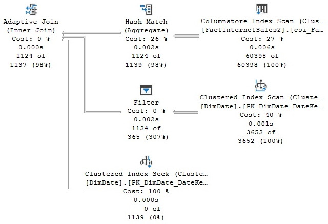
Figure 11.4 – A plan using a Columnstore Index Scan operator in batch mode

Note

Older versions of SQL Server required a large number of rows in order to run in batch execution mode. Even when they were able to use the columnstore index, a small table could only use row execution mode.

You can validate on the properties of the Columnstore Index Scan operator that the Actual Execution Mode value is Batch (see Figure 11.5). In the same way, the Storage property shows ColumnStore:

Figure 11.5 – The Columnstore Index Scan properties

Similar to a rowstore, you can use the ALTER INDEX REBUILD statement to remove any fragmentation of a columnstore index, as shown in the following code:

ALTER INDEX csi_FactInternetSales2 on FactInternetSales2 REBUILD

Because a fact table is a very large table, and an index rebuild operation in a columnstore index is an offline operation, you can partition it and follow the same recommendations you would for a large table in a rowstore. Here is a basic summary of the process:

• Rebuild the most recently used partition only. Fragmentation is more likely to occur only in partitions that have been modified recently.
• Rebuild only the partitions that have been updated after loading data or heavy DML operations.

Similar to dropping a regular clustered index, dropping a clustered columnstore index will convert the table back into a rowstore heap. To verify this, run the following query:

SELECT * FROM sys.indexes

WHERE object_id = OBJECT_ID(‘FactInternetSales2’)

An output similar to the following will be shown:

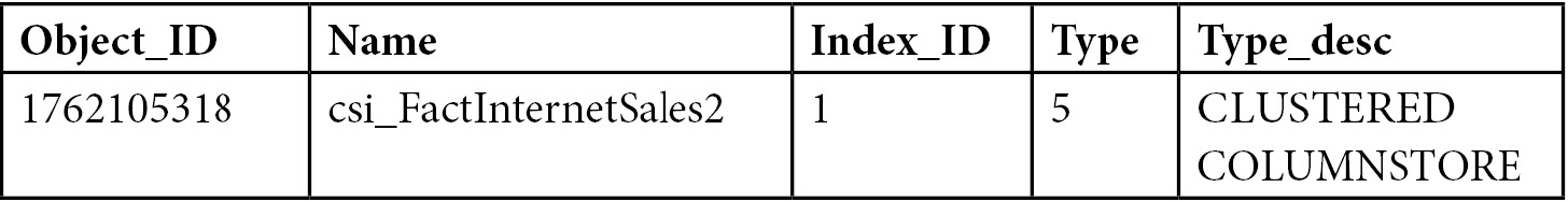
Dropping the index running by using the next DROP INDEX statement and then running the previous query again will change index_id to 0 and type_desc to HEAP:

DROP INDEX FactInternetSales2.csi_FactInternetSales2

Hints

Finally, a couple of hints could be useful in cases where the query optimizer is not giving you a good plan when working with nonclustered columnstore indexes. One case is when the query optimizer ignores this index. In this case, you can use the INDEX hint to ask SQL Server to use the existing nonclustered columnstore index. To test it, create the following index in the existing FactInternetSales table:

CREATE NONCLUSTERED COLUMNSTORE INDEX csi_FactInternetSales

ON dbo.FactInternetSales (

ProductKey,

OrderDateKey,

DueDateKey,

ShipDateKey,

CustomerKey,

PromotionKey,

CurrencyKey,

SalesTerritoryKey,

SalesOrderNumber,

SalesOrderLineNumber,

RevisionNumber,

OrderQuantity,

UnitPrice,

ExtendedAmount,

UnitPriceDiscountPct,

DiscountAmount,

ProductStandardCost,

TotalProductCost,

SalesAmount,

TaxAmt,

Freight,

CarrierTrackingNumber,

CustomerPONumber,

OrderDate,

DueDate,

ShipDate

)

Assuming the columnstore index is not selected in the final execution plan, you could use the INDEX hint in the following way:

SELECT d.CalendarYear,

SUM(SalesAmount) AS SalesTotal

FROM dbo.FactInternetSales AS f

WITH (INDEX(csi_FactInternetSales))

JOIN dbo.DimDate AS d

ON f.OrderDateKey = d.DateKey

GROUP BY d.CalendarYear

ORDER BY d.CalendarYear

Another case is when for some reason you don’t want to use an existing nonclustered columnstore index. In this case, the IGNORE_NONCLUSTERED_COLUMNSTORE_INDEX hint could be used, as shown in the following query:

SELECT d.CalendarYear,

SUM(SalesAmount) AS SalesTotal

FROM dbo.FactInternetSales AS f

JOIN dbo.DimDate AS d

ON f.OrderDateKey = d.DateKey

GROUP BY d.CalendarYear

ORDER BY d.CalendarYear

OPTION (IGNORE_NONCLUSTERED_COLUMNSTORE_INDEX)

Finally, drop the created columnstore index by running the following statement:

DROP INDEX FactInternetSales.csi_FactInternetSales

Summary

This chapter covered data warehouses and explained how operational and analytic systems serve very different purposes—one helping with the execution of a business process and the other helping with the measurement of such a business process. The fact that a data warehouse system is also used differently from an OLTP system created opportunities for a new database engine design, which was implemented using the columnstore indexes feature when SQL Server 2012 was originally released.

Because a typical star join query only uses between 10 percent and 15 percent of the columns in a fact table, a columnar-based approach was implemented, which seemed to be more appropriate than the traditional rowstore. Because processing one row at a time also did not seem to be efficient for the large number of rows processed by star join queries, a new batch-processing mode was implemented, too. Finally, following new hardware trends, columnstore indexes, same as with in-memory OLTP, were implemented as in-memory technologies.

Additionally. the SQL Server query optimizer is able to automatically detect and optimize data warehouse queries. One of the explained optimizations, using bitmap filtering, is based on a concept originally conceived in 1970. Bitmap filtering can be used to filter out rows from a fact table very early during query processing, thus improving the performance of star join queries. In the next and final chapter, we will learn how to understand various query hints.