Chapter 7: In-Memory OLTP

Relational database management systems (RDBMSs) were originally architected in the late 1970s. Since the hardware was vastly different in those days, recently, there has been extensive research in the database community indicating that a new design and architectural approach should be required for the hardware available today.

RDBMSs were originally designed under the assumption that computer memory was limited and expensive and that databases were many times larger than the main memory. Because of that, it was decided that data should reside on disk. With current hardware having memory sizes and disk volumes thousands of times larger, and processors thousands of times faster, these assumptions are no longer true. In addition, disk access has been subject to physical limits since its introduction; it has not increased at a similar pace and continues to be the slowest part of the system. Although memory capacity has grown dramatically – which is not the case for the size of OLTP databases – one of the new design considerations is that an OLTP engine should be memory-based instead of disk-oriented since most OLTP databases can now fit into the main memory.

In addition, research performed early on for the Hekaton project at Microsoft showed that even with the current hardware available today, a 10 to 100 times performance improvement could not be achieved using current SQL Server mechanisms; instead, it would require dramatically changing the way data management systems are designed. SQL Server is already highly optimized, so using existing techniques could not deliver dramatic performance gains or orders of magnitude speedup. Even after the main memory engine was built, there was still significant time spent in query processing, so they realized they needed to drastically reduce the number of instructions executed. Taking advantage of available memory is not just a matter of reading more of the existing disk pages to memory – it involves redesigning data management systems using a different approach to gain the most benefit from this new hardware. Finally, standard concurrency control mechanisms available today do not scale up to the high transaction rates achievable by an in-memory-optimized database, so locking becomes the next bottleneck.

Specialized in-memory database engines have appeared on the market in the last two decades, including Oracle TimesTen and IBM solidDB. Microsoft also started shipping in-memory technologies with the xVelocity in-memory analytics engine as part of SQL Server Analysis Services and the xVelocity memory-optimized columnstore indexes integrated into the SQL Server database engine. In-memory OLTP, code-named Hekaton, was introduced in SQL Server 2014 as a new OLTP in-memory database engine. Hekaton’s performance improvement is based on three major architecture areas: optimization for main memory access, compiling procedures to native code, and lock and latches elimination. We will look at these three major areas in this chapter.

In this chapter, we cover Hekaton. xVelocity memory-optimized columnstore indexes will be covered in Chapter 11, An Introduction to Data Warehouses. To differentiate the Hekaton engine terminology from the standard SQL Server engine covered in the rest of this book, this chapter will call Hekaton tables and stored procedures memory-optimized tables and natively compiled stored procedures, respectively. Standard tables and procedures will be called disk-based tables and regular or interpreted stored procedures, respectively.

This chapter covers the following topics:

• In-memory OLTP architecture
• Tables and indexes
• Natively compiled stored procedures
• Limitations and later enhancements

In-memory OLTP architecture

One of the main strategic decisions made during the Hekaton project was to build a new database engine fully integrated into SQL Server instead of creating a new, separate product as other vendors did. This gave users several advantages, such as enabling existing applications to run without code changes, and not needing to buy and learn about a separate product. As mentioned earlier, Hekaton can provide a several orders of magnitude performance increase based on the following:

• Optimized tables and indexes for main memory data access: Hekaton tables and indexes are designed and optimized for memory. They are not stored as database pages, and they do not use a memory buffer pool either.
• T-SQL modules compiled to native code: Stored procedures can be optimized by the SQL Server query optimizer, like any regular stored procedure, and then compiled into highly efficient machine code. When this happens, trigger and scalar user-defined functions can also be natively compiled.
• Locks and latches elimination: Hekaton implements a new optimistic multiversion concurrency control (MVCC) mechanism, which uses new data structures to eliminate traditional locks and latches, so there is no waiting because of blocking.

Note

In-memory OLTP was mostly known as Hekaton in its first few years and the name was used extensively in many texts and documents, including the first edition of this book. We will try to use in-memory OLTP as much as possible in the rest of this chapter.

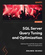
The lack of a locking and latching mechanism does not mean that chaos will ensue as in-memory OLTP uses MVCC to provide snapshots, repeatable read, and serializable transaction isolation, as covered later. The Hekaton database engine has three major components, as shown in the following diagram:

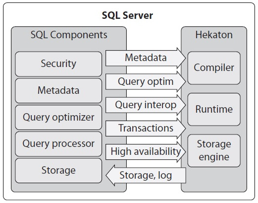
Figure 7.1 – The Hekaton database engine

The three major components are as follows:

• Hekaton storage engine: This component manages tables and indexes while providing support for storage, transactions, recoverability, high availability, and so on.
• Hekaton compiler: This component compiles procedures and tables into native code, which are loaded as DLLs into the SQL Server process.
• Hekaton runtime system: This component provides integration with other SQL Server resources.

Hekaton memory-optimized tables are stored in memory using new data structures that are completely different from traditional disk-based tables. They are also kept on disk but only for durability purposes, so they are only read from disk during database recovery, such as when the SQL Server instance starts. In-memory OLTP tables are fully ACID – that is, they guarantee the Atomicity, Consistency, Isolation, and Durability properties – although a nondurable version of the tables is available as well, in which data is not persisted on disk. Memory-optimized tables must have at least one index, and there is no data structure equivalent to a heap. SQL Server uses the same transaction log as the normal engine to log operations for both disk-based and memory-optimized tables, but in-memory transaction log records are optimized and consume less overall log space. In-memory OLTP indexes are only maintained in memory, so they are never persisted on disk. Consequently, their operations are never logged. Indexes are rebuilt when data is loaded into memory at SQL Server restart.

Although natively compiled stored procedures can only access memory-optimized tables, SQL Server provides operators for accessing and updating Hekaton tables, which can be used by interpreted T-SQL. This functionality is provided by a new component called the query interop, which also allows you to access and update both memory-optimized and regular tables in the same transaction.

In-memory OLTP can help in applications experiencing CPU, I/O, and locking bottlenecks. By using natively compiled stored procedures, fewer instructions are executed than with a traditional stored procedure, thus helping in cases where the execution time is dominated by the stored procedure code. Except for logging, no I/O is required during normal database operations, and Hekaton even requires less logging than operations with regular disk-based tables. Applications with concurrency issues, such as contention in locks, latches, and spinlocks, can also greatly benefit from Hekaton because it does not use locks and latches when accessing data.

Note

A particular scenario where in-memory OLTP can greatly improve performance is in the so-called last-page insert problem on traditional tables. This problem happens when latch contention is caused. This is when many threads continually attempt to update the last page of an index due to the use of incremental keys. By eliminating latches and locks, Hekaton can make these operations extremely fast.

However, in-memory OLTP cannot be used to improve performance if your application has memory or network bottlenecks. Hekaton requires that all the tables defined as memory-optimized actually fit in memory, so your installation must have enough RAM to fit them all.

Finally, Hekaton was originally only available in the 64-bit version of SQL Server 2014 and was an Enterprise Edition-only feature. However, starting with SQL Server 2016 Service Pack 1, in-memory OLTP, along with all the application and programmability features of SQL Server, has been available on all the editions of the product, including Express and Standard. Also, starting with the 2016 release, SQL Server is only available for the 64-bit architecture.

Now that we have a better understanding of the in-memory OLTP architecture, let’s start looking at the technology.

Tables and indexes

As explained earlier, Hekaton tables can be accessed either by natively compiled stored procedures or by standard T-SQL, such as ad hoc queries or standard stored procedures. Tables are stored in memory, and each row can potentially have multiple versions. Versions are kept in memory instead of tempdb, which is what the versioning mechanism of the standard database engine uses. Versions that are no longer needed – that is, that are no longer visible to any transaction – are deleted to avoid filling up the available memory. This process is known as garbage collection.

Chapter 5, Working with Indexes, introduced indexes for traditional tables. Memory-optimized tables also benefit from indexes, and in this section, we will talk about these indexes and how they are different from their disk-based counterparts. As explained earlier, Hekaton indexes are never persisted to disk; they only exist in memory, and because of that, their operations are not logged in the transaction log. Only index metadata is persisted, and indexes are rebuilt when data is loaded into memory at SQL Server restart.

Two different kinds of indexes exist on Hekaton: hash and range indexes, both of which are lock-free implementations. Hash indexes support index seeks on equality predicates, but they cannot be used with inequality predicates or to return sorted data. Range indexes can be used for range scans, ordered scans, and operations with inequality predicates. Range indexes can also be used for index seeks on equality predicates, but hash indexes offer far better performance and are the recommended choice for this kind of operation.

Note

Range indexes are called nonclustered indexes or memory-optimized nonclustered indexes in the latest updates of the SQL Server documentation. Keep that in mind in case range indexes is no longer used in future documentation.

Hash indexes are not ordered indexes; scanning them would return records in random order. Both kinds of indexes are covering indexes; the index contains memory pointers to the table rows where all the columns can be retrieved. You cannot directly access a record without using an index, so at least one index is required to locate the data in memory.

Although the concepts of fragmentation and fill factor, as explained in Chapter 5, Working with Indexes, do not apply to Hekaton indexes, we may see that we can get similar but new behavior with the bucket count configuration: a hash index can have empty buckets, resulting in wasted space that impacts the performance of index scans, or there might be a large number of records in a single bucket, which may impact the performance of search operations. In addition, updating and deleting records can create a new kind of fragmentation on the underlying data disk storage.

Creating in-memory OLTP tables

Creating a memory-optimized table requires a memory-optimized filegroup. The following error is returned if you try to create a table and you do not have one:

Msg 41337, Level 16, State 0, Line 1

Cannot create memory optimized tables. To create memory optimized tables, the database must have a MEMORY_OPTIMIZED_FILEGROUP that is online and has at least  one container.

You can either create a new database with a memory-optimized filegroup or add one to an existing database. The following statement shows the first scenario:

CREATE DATABASE Test

ON PRIMARY (NAME = Test_data,

FILENAME = 'C:DATATest_data.mdf', SIZE=500MB),

FILEGROUP Test_fg CONTAINS MEMORY_OPTIMIZED_DATA

(NAME = Test_fg, FILENAME = 'C:DATATest_fg')

LOG ON (NAME = Test_log, Filename='C:DATATest_log.ldf', SIZE=500MB)

COLLATE Latin1_General_100_BIN2

Note that in the preceding code, a C:Data folder is being used; change this as appropriate for your installation. The following code shows how to add a memory-optimized data filegroup to an existing database:

CREATE DATABASE Test

ON PRIMARY (NAME = Test_data,

FILENAME = 'C:DATATest_data.mdf', SIZE=500MB)

LOG ON (NAME = Test_log, Filename='C:DATATest_log.ldf', SIZE=500MB)

GO

ALTER DATABASE Test ADD FILEGROUP Test_fg CONTAINS MEMORY_OPTIMIZED_DATA

GO

ALTER DATABASE Test ADD FILE (NAME = Test_fg, FILENAME = N'C:DATATest_fg')

TO FILEGROUP Test_fg

GO

Note

You may have noticed that the first CREATE DATABASE statement has a COLLATE clause but the second does not. There were some collation restrictions on the original release that were lifted on SQL Server 2016. More details on this can be found at the end of this chapter.

Once you have a database with a memory-optimized filegroup, you are ready to create your first memory-optimized table. For this exercise, you will copy data from AdventureWorks2019 to the newly created Test database. You may notice that scripting any of the AdventureWorks2019 tables and using the resulting code to create a new memory-optimized table will immediately show the first limitation of Hekaton: not all table properties were supported on the initial release, as we will see later. You could also use Memory Optimization Advisor to help you migrate disk-based tables to memory-optimized tables.

Note

You can run Memory Optimization Advisor by right-clicking a table in SQL Server Management Studio and selecting it from the available menu choices. In the same way, you can run Native Compilation Advisor by right-clicking any stored procedure you want to convert into native code.

Creating a memory-optimized table requires the MEMORY_OPTIMIZED clause, which needs to be set to ON. Explicitly defining DURABILITY as SCHEMA_AND_DATA is also recommended, although this is its default value if the DURABILITY clause is not specified.

Using our new Test database, you can try to create a table that only defines MEMORY_OPTIMIZED, as shown here:

CREATE TABLE TransactionHistoryArchive (

TransactionID int NOT NULL,

ProductID int NOT NULL,

ReferenceOrderID int NOT NULL,

ReferenceOrderLineID int NOT NULL,

TransactionDate datetime NOT NULL,

TransactionType nchar(1) NOT NULL,

Quantity int NOT NULL,

ActualCost money NOT NULL,

ModifiedDate datetime NOT NULL

) WITH (MEMORY_OPTIMIZED = ON)

However, you will get the following error:

Msg 41321, Level 16, State 7, Line 1

The memory optimized table 'TransactionHistoryArchive' with

DURABILITY=SCHEMA_AND_DATA must have a primary key.

Msg 1750, Level 16, State 0, Line 1

Could not create constraint or index. See previous errors.

Because this error indicates that a memory-optimized table must have a primary, you could define one by changing the following line:

TransactionID int NOT NULL PRIMARY KEY,

However, you will still get the following message:

Msg 12317, Level 16, State 76, Line 17

Clustered indexes, which are the default for primary keys, are not supported with memory optimized tables.

Change the previous line so that it specifies a nonclustered index:

TransactionID int NOT NULL PRIMARY KEY NONCLUSTERED,

The statement will finally succeed and create a table with a range or nonclustered index.

A hash index can also be created for the primary key if you explicitly use the HASH clause, as specified in the following example, which also requires the BUCKET_COUNT option. First, let’s drop the new table by using DROP TABLE in the same way as with a disk-based table:

DROP TABLE TransactionHistoryArchive

Then, we can create the table:

CREATE TABLE TransactionHistoryArchive (

TransactionID int NOT NULL PRIMARY KEY NONCLUSTERED HASH WITH

(BUCKET_COUNT = 100000),

ProductID int NOT NULL,

ReferenceOrderID int NOT NULL,

ReferenceOrderLineID int NOT NULL,

TransactionDate datetime NOT NULL,

TransactionType nchar(1) NOT NULL,

Quantity int NOT NULL,

ActualCost money NOT NULL,

ModifiedDate datetime NOT NULL

) WITH (MEMORY_OPTIMIZED = ON)

Note

The initial release of in-memory OLTP did not allow a table to be changed. You would need to drop the table and create it again to implement any changes. Starting with SQL Server 2016, you can use the ALTER TABLE statement to achieve that. More details can be found at the end of this chapter.

So, a memory-optimized table must also have a primary key, which could be a hash or a range index. The maximum number of indexes was originally limited to eight, but starting with SQL Server 2017, Microsoft has removed this limitation. But the same as with disk-based indexes, you should keep the number of indexes to a minimum. We can have both hash and range indexes on the same table, as shown in the following example (again, dropping the previous table if needed):

CREATE TABLE TransactionHistoryArchive (

TransactionID int NOT NULL PRIMARY KEY NONCLUSTERED HASH WITH

(BUCKET_COUNT = 100000),

ProductID int NOT NULL,

ReferenceOrderID int NOT NULL,

ReferenceOrderLineID int NOT NULL,

TransactionDate datetime NOT NULL,

TransactionType nchar(1) NOT NULL,

Quantity int NOT NULL,

ActualCost money NOT NULL,

ModifiedDate datetime NOT NULL,

INDEX IX_ProductID NONCLUSTERED (ProductID)

) WITH (MEMORY_OPTIMIZED = ON)

The preceding code creates a hash index on the TransactionID column, which is also the table’s primary key, and a range index on the ProductID column. The NONCLUSTERED keyword is optional for range indexes in this example. Now that the table has been created, we are ready to populate it by copying data from AdventureWorks2019. However, the following will not work:

INSERT INTO TransactionHistoryArchive

SELECT * FROM AdventureWorks2019.Production.TransactionHistoryArchive

We will get the following error message:

Msg 41317, Level 16, State 3, Line 1

A user transaction that accesses memory optimized tables or natively compiled procedures cannot access more than one user database or databases model and msdb, and it cannot write to master.

As indicated in the error message, a user transaction that accesses memory-optimized tables cannot access more than one user database. For the same reason, the following code for joining two tables from two user databases will not work either:

SELECT * FROM TransactionHistoryArchive tha

JOIN AdventureWorks2019.Production.TransactionHistory ta

ON tha.TransactionID = ta.TransactionID

However, you can copy this data in some other ways, such as using the Import and Export Wizard or using a temporary table, as shown in the following code:

SELECT * INTO #temp

FROM AdventureWorks2019.Production.TransactionHistoryArchive

GO

INSERT INTO TransactionHistoryArchive

SELECT * FROM #temp

However, as explained earlier, a user transaction that’s accessing memory-optimized tables and disk-based tables on the same database is supported (except in the case of natively compiled stored procedures). The following example will create a disk-based table and join both a memory-optimized and a disk-based table:

CREATE TABLE TransactionHistory (

TransactionID int,

ProductID int)

GO

SELECT * FROM TransactionHistoryArchive tha

JOIN TransactionHistory ta ON tha.TransactionID = ta.TransactionID

As shown earlier, the minimum requirement to create a memory-optimized table is to use the MEMORY_OPTIMIZED clause and define a primary key, which itself requires an index. A second and optional clause, DURABILITY, is also commonly used and supports the SCHEMA_AND_DATA and SCHEMA_ONLY options. SCHEMA_AND_DATA, which is the default, allows both schema and data to be persisted on disk. SCHEMA_ONLY means that the table data will not be persisted on disk upon instance restart; only the table schema will be persisted. SCHEMA_ONLY creates nondurable tables, which can improve the performance of transactions by significantly reducing the I/O impact of the workload. This can be used in scenarios such as session state management and staging tables that are used in ETL processing.

The following diagram shows the structure of a record in a memory-optimized table in which we can identify two main parts: a row header and a row body or payload. The row header starts with a begin and end timestamp, which is used to identify where the record is valid for a transaction, as explained later in this section:

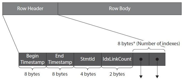
Figure 7.2 – Structure of a Hekaton row

Next is StmtId, which is the statement ID value of the statement that created the row. The last section of the header consists of index pointers, one per index available on the table. The row body is the record itself and contains the index key columns, along with the remaining columns of the row. Because the row body contains all the columns of the record, we could say that, in Hekaton, there is no need to define covering indexes as with traditional indexes: a memory-optimized index is a covering index, meaning that all the columns are included in the index. An index contains a memory pointer to the actual row in the table.

Now, let’s review hash and nonclustered (range) indexes in more detail.

Hash indexes

Hash indexes were introduced previously. Now, let’s look at them in more detail. The following diagram shows an example of hash indexes containing three records: the Susan row, the Jane row, and the John row. Notice that John has two versions, the complexities and relationships of which will be explained shortly. Two hash indexes are defined: the first on the Name column and the second on the City column, so a hash table is allocated for each index, with each box representing a different hash bucket. The first part of the record (for example, 90, 150) is the begin and end timestamp shown previously in Figure 7.2. The infinity symbol (∞) at the end timestamp means that this is the currently valid version of the row. For simplicity, this example assumes that each hash bucket contains records based on the first letter of the key, either Name or City, although this is not how the hash function works, as explained later:

Figure 7.3 – Example of Hekaton rows and indexes

Because the table has two indexes, each record has two pointers, one for each index, as shown in Figure 7.2. The first hash bucket for the Name index has a chain of three records: two versions for John and one version for Jane. The links between these records are shown with gray arrows. The second hash bucket for the Name index only has a chain of one record – the Susan record – so no links are shown. In the same way, the preceding diagram shows two buckets for the City index – the first with two records for Beijing and Bogota, and the second for Paris and Prague. The links are shown in black arrows. The John, Beijing record has a valid time from 200 to infinity, which means it was created by a transaction that was committed at time 200 and the record is still valid. The other version (John, Paris) was valid from time 100 to 200, when it was updated to John, Beijing. In the MVCC system, UPDATEs are treated as INSERTs and DELETEs. Rows are only visible from the begin timestamp and up until (but not including) the end timestamp, so in this case, the existing version was expired by setting the end timestamp, and a new version with an infinity end timestamp was created.

A transaction that was started at time 150 would then see the John, Paris version, while one started at 220 would find the latest version of John, Beijing. But how does SQL Server find the records using the index? This is where the hash function comes into play.

For the statement, we will use the following code:

SELECT * FROM Table WHERE City = 'Beijing'

SQL Server will apply the hash function to the predicate. Remember that for simplicity, our hash function example was based on the first letter of the string, so in this case, the result is B. SQL Server will then look directly into the hash bucket and pull the pointer to the first row. Looking at the first row, it will now compare the strings; if they are the same, it will return the required row details. Then, it will walk the chain of index pointers, comparing the values and returning rows where appropriate.

Finally, notice that the example uses two hash indexes, but the same example would work if we had used, for example, a hash index on Name and a range index on City, or both range indexes.

BUCKET_COUNT controls the size of the hash table, so this value should be chosen carefully. The recommendation is to have it twice the maximum expected number of distinct values in the index key, rounded up to the nearest power of two, although Hekaton will round up for you if needed. An inadequate BUCKET_COUNT value can lead to performance problems: a value too large can lead to many empty buckets in the hash table. This can cause higher memory usage as each bucket uses 8 bytes. Also, scanning the index will be more expensive because it has to scan those empty buckets. However, a large BUCKET_COUNT value does not affect the performance of index seeks. On the other hand, a BUCKET_COUNT value that’s too small can lead to long chains of records that will cause searching for a specific record to be more expensive. This is because the engine has to traverse multiple values to find a specific row.

Let’s see some examples of how BUCKET_COUNT works, starting with an empty table. Drop the existing TransactionHistoryArchive table:

DROP TABLE TransactionHistoryArchive

Now, create the table again with a BUCKET_COUNT of 100,000:

CREATE TABLE TransactionHistoryArchive (

TransactionID int NOT NULL PRIMARY KEY NONCLUSTERED HASH WITH

(BUCKET_COUNT = 100000),

ProductID int NOT NULL,

ReferenceOrderID int NOT NULL,

ReferenceOrderLineID int NOT NULL,

TransactionDate datetime NOT NULL,

TransactionType nchar(1) NOT NULL,

Quantity int NOT NULL,

ActualCost money NOT NULL,

ModifiedDate datetime NOT NULL

) WITH (MEMORY_OPTIMIZED = ON)

You can use the sys.dm_db_xtp_hash_index_stats DMV to show statistics about hash indexes. Run the following code:

SELECT * FROM sys.dm_db_xtp_hash_index_stats

You will get the following output:

Here, we can see that instead of 100,000 buckets, SQL Server rounded up to the nearest power of two (in this case, 2 ^ 17, or 131,072), as shown in the total_bucket_count column.

Insert the same data again by running the following statements:

DROP TABLE #temp

GO

SELECT * INTO #temp

FROM AdventureWorks2019.Production.TransactionHistoryArchive

GO

INSERT INTO TransactionHistoryArchive

SELECT * FROM #temp

This time, 89,253 records have been inserted. Run the sys.dm_db_xtp_hash_index_stats DMV again. This time, you will get data similar to the following:

We can note several things here. The total number of buckets (131,072) minus the empty buckets (66,316), shown as empty_bucket_count, gives us the number of buckets used (64,756). Because we inserted 89,253 records in 39,191 buckets, this gives us 1.37 records per bucket on average, which is represented by the avg_chain_len value of 1, documented as the average length of the row chains over all the hash buckets in the index. max_chain_len is the maximum length of the row chains in the hash buckets.

Just to show an extreme case where performance may be impaired, run the same exercise, but request only 1,024 as BUCKET_COUNT. After inserting the 89,253 records, we will get the following output:

In this case, we have 89,253 records divided by 1,024 (or 87.16 records per bucket). Hash collisions occur when two or more index keys are mapped to the same hash bucket, as in this example, and a large number of hash collisions can impact the performance of lookup operations.

The other extreme case is having too many buckets compared to the number of records. Running the same example for 1,000,000 buckets and inserting the same number of records would give us this:

This example has 91.79% unused buckets, which will both use more memory and impact the performance of scan operations because of it having to read many unused buckets.

Are you wondering what the behavior will be if we have the same number of buckets as records? Change the previous code to create 65,536 buckets. Then, run the following code:

DROP TABLE #temp

GO

SELECT TOP 65536 * INTO #temp

FROM AdventureWorks2019.Production.TransactionHistoryArchive

GO

INSERT INTO TransactionHistoryArchive

SELECT * FROM #temp

You will get the following output:

So, after looking at these extreme cases, it is worth reminding ourselves that the recommendation is to configure BUCKET_COUNT as twice the maximum expected number of distinct values in the index key, keeping in mind that changing BUCKET_COUNT is not a trivial matter and requires the table to be dropped and recreated.

SQL Server uses the same hashing function for all the hash indexes. It is deterministic, which means that the same index key will always be mapped to the same bucket in the index. Finally, as we were able to see in the examples, multiple index keys can also be mapped to the same hash bucket, and because key values are not evenly distributed in the buckets, there can be several empty buckets, and used buckets may contain one or more records.

Nonclustered or range indexes

Although hash indexes support index seeks on equality predicates and are the best choice for point lookups, the index seeks on inequality predicates, like the ones that use the >, <, <=, and >= operators, are not supported on this kind of index. So, an inequality predicate will skip a hash index and use a table scan instead. In addition, because all the index key columns are used to compute the hash value, index seeks on a hash index cannot be used when only a subset of these index key columns are used in an equality predicate. For example, if the hash index is defined as lastname, firstname, you cannot use it in an equality predicate using only lastname or only firstname. Hash indexes cannot be used to retrieve the records sorted by the index definition either.

Range indexes can be used to help in all these scenarios and have the additional benefit that they do not require you to define several buckets. However, although range indexes have several advantages over hash indexes, keep in mind that range indexes could lead to suboptimal performance for index seek operations, where hash indexes are recommended instead.

Range indexes are a new form of B-tree, called a Bw-tree, and are designed for new hardware to take advantage of the cache of modern multicore processors. They are in-memory structures that achieve outstanding performance via latch-free techniques and were originally described by Microsoft Research in the paper The Bw-Tree: A B-tree for New Hardware Platforms, by Justin Levandoski and others. The following diagram shows the general structure of a Bw-tree:

Figure 7.4 – Structure of a Bw-tree

Similar to a regular B-tree, as explained in Chapter 5, Working with Indexes, in a Bw-tree, the root and non-leaf pages point to index pages at the next level of the tree, and the leaf pages contain a set of ordered key values with pointers that point to the data rows. Each non-leaf page has a logical page ID (PID), and a page mapping table contains the mapping of these PIDs to their physical memory address. For example, in the preceding diagram, the top entry of the page mapping table specifies the number 0 and points to the page with PID 0. Keys on non-leaf pages contain the highest value possible that this page references. Leaf pages do not have a PID, only memory addresses pointing to the data rows. So, to find the row with a key equal to 2, SQL Server would start with the root page (PID 0), follow the link for key = 10 (because 10 is greater than 2), which points to the page with PID 3, and then follow the link for key = 5 (which again is greater than 2). The pointed leaf page contains key 2, which contains the memory address that points to the required record. For more details about the internals of these new memory structures, you may want to refer to the research paper listed previously.

Now, let’s run some queries to get a basic understanding of how these indexes work and what kind of execution plans they create. In this section, we will use ad hoc T-SQL, which in Hekaton is said to use query interop capabilities. The examples in this section use the following table with both a hash and a range index. Also, you must load data into this table, as explained previously:

CREATE TABLE TransactionHistoryArchive (

TransactionID int NOT NULL PRIMARY KEY NONCLUSTERED HASH WITH

(BUCKET_COUNT = 100000),

ProductID int NOT NULL,

ReferenceOrderID int NOT NULL,

ReferenceOrderLineID int NOT NULL,

TransactionDate datetime NOT NULL,

TransactionType nchar(1) NOT NULL,

Quantity int NOT NULL,

ActualCost money NOT NULL,

ModifiedDate datetime NOT NULL,

INDEX IX_ProductID NONCLUSTERED (ProductID)

) WITH (MEMORY_OPTIMIZED = ON)

First, run the following query:

SELECT * FROM TransactionHistoryArchive

WHERE TransactionID = 8209

Because we defined a hash index on the TransactionID column, we get the plan shown here, which uses an Index Seek operator:

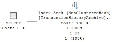
Figure 7.5 – Index Seek operation on a hash index

The index is named PK__Transact__55433A4A7EB94404. This name was given automatically but it is also possible to specify a name, if required, as you’ll see later. As mentioned previously, hash indexes are efficient for point lookups, but they do not support index seeks on inequality predicates. If you change the previous query so that it uses an inequality predicate, as shown here, it will create a plan with a Table Scan, as shown in the following plan:

SELECT * FROM TransactionHistoryArchive

WHERE TransactionID > 8209

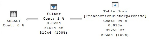
Figure 7.6 – Index Scan operation on a hash index

Now, let’s try a different query:

SELECT * FROM TransactionHistoryArchive

WHERE ProductID = 780

Because we have a range nonclustered index defined on ProductID, an Index Seek operation will be used on that index, IX_ProductID, as shown here:

Figure 7.7 – Index Seek operation on a range index

Now, let’s try an inequality operation on the same column:

SELECT * FROM TransactionHistoryArchive

WHERE ProductID < 10

This time, the range index can be used to access the data, without the need for an Index Scan operation. The resulting plan can be seen here:

Figure 7.8 – Index Seek operation on a range index with an inequality predicate

Hash indexes cannot be used to return data that’s been sorted because their rows are stored in a random order. The following query will use a Sort operation to sort the requested data, as shown in the following plan:

SELECT * FROM TransactionHistoryArchive

ORDER BY TransactionID

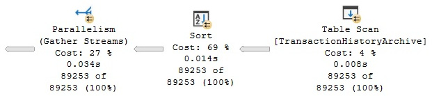
Figure 7.9 – Plan with a Sort operation

However, a range index can be used to return sorted data. Running the following query will simply scan the range index without the need for it to sort its data, as shown in the following plan. You could even verify that the Ordered property is True via the operator properties:

SELECT * FROM TransactionHistoryArchive

ORDER BY ProductID

Figure 7.10 – Using a range index to return sorted data

However, unlike disk-based indexes, range indexes are unidirectional, which is something that may surprise you. Therefore, when requesting the same query using ORDER BY ProductID DESC, it will not be able to use the index-sorted data. Instead, it will use a plan with an expensive Sort operator, similar to the one shown in Figure 7.9.

Finally, let’s look at an example of a hash index with two columns. Let’s assume you have the following version of the TransactionHistoryArchive table, which uses a hash index with both TransactionID and ProductID columns. Once again, load some data into this table, as explained earlier:

CREATE TABLE TransactionHistoryArchive (

TransactionID int NOT NULL,

ProductID int NOT NULL,

ReferenceOrderID int NOT NULL,

ReferenceOrderLineID int NOT NULL,

TransactionDate datetime NOT NULL,

TransactionType nchar(1) NOT NULL,

Quantity int NOT NULL,

ActualCost money NOT NULL,

ModifiedDate datetime NOT NULL,

CONSTRAINT PK_TransactionID_ProductID PRIMARY KEY NONCLUSTERED

HASH (TransactionID, ProductID) WITH (BUCKET_COUNT = 100000)

) WITH (MEMORY_OPTIMIZED = ON)

Because all the index key columns are required to compute the hash value, as explained earlier, SQL Server will be able to use a very effective Index Seek on the PK_TransactionID_ProductID hash index in the following query:

SELECT * FROM TransactionHistoryArchive

WHERE TransactionID = 7173 AND ProductID = 398

However, it will not be able to use the same index in the following query, which will resort to a Table Scan:

SELECT * FROM TransactionHistoryArchive

WHERE TransactionID = 7173

Although the execution plans shown in this section use the familiar Index Scan and Index Seek operations, keep in mind that these indexes and the data are in memory and there is no disk access at all. In this case, the table and indexes are in memory and use different structures. So, how do you identify them when you see them in execution plans, especially when you query both memory-optimized and disk-based tables? You can look at the Storage property in the operator details and see a value of MemoryOptimized. Although you will see NonClusteredHash after the name of the operator for hash indexes, range indexes just show NonClustered, which is the same that’s shown for regular disk-based nonclustered indexes.

Natively compiled stored procedures

As mentioned previously, to create natively compiled stored procedures, Hekaton leverages the SQL Server query optimizer to produce an efficient query plan, which is later compiled into native code and loaded as DLLs into the SQL Server process. You may want to use natively compiled stored procedures mostly in performance-critical parts of an application or in procedures that are frequently executed. However, you need to be aware of the limitations of the T-SQL-supported features on natively compiled stored procedures. These will be covered later in this chapter.

Creating natively compiled stored procedures

Now, let’s create a natively compiled stored procedure that, as shown in the following example, requires the NATIVE_COMPILATION clause:

CREATE PROCEDURE test

WITH NATIVE_COMPILATION, SCHEMABINDING, EXECUTE AS OWNER

AS

BEGIN ATOMIC WITH (TRANSACTION ISOLATION LEVEL = SNAPSHOT,

LANGUAGE = 'us_english')

SELECT TransactionID, ProductID, ReferenceOrderID

FROM dbo.TransactionHistoryArchive

WHERE ProductID = 780

END

After creating the procedure, you can execute it by using the following command:

EXEC test

You can display the execution plan that’s being used by clicking Display Estimated Execution Plan or using the SET SHOWPLAN_XML ON statement. If you run this against the first table that was created in the Nonclustered or range indexes section, you will get the following plan:

Figure 7.11 – Execution plan of a natively compiled stored procedure

In addition to NATIVE_COMPILATION, the code shows other required clauses: SCHEMABINDING, EXECUTE AS, and BEGIN ATOMIC. Leaving any of these out will produce an error. These choices must be set at compile time and aim to minimize the number of runtime checks and operations that must be performed at execution time, thus helping with the performance of the execution.

SCHEMABINDING refers to the fact that natively compiled stored procedures must be schema bound, which means that tables referenced by the procedure cannot be dropped. This helps to avoid costly schema stability locks before execution. Trying to delete the dbo.TransactionHistoryArchive table we created earlier would produce the following error:

Msg 3729, Level 16, State 1, Line 1

Cannot DROP TABLE 'dbo.TransactionHistoryArchive' because it is being referenced by object 'test'.

The EXECUTE AS requirement focuses on avoiding permission checks at execution time. In natively compiled stored procedures, the default of EXECUTE AS CALLER is not supported, so you must use any of the other three choices available: EXECUTE AS SELF, EXECUTE AS OWNER, or EXECUTE AS user_name.

BEGIN ATOMIC is part of the ANSI SQL standard, and in SQL Server, it’s used to define an atomic block in which either the entire block succeeds or all the statements in the block are rolled back. If the procedure is invoked outside the context of an active transaction, BEGIN ATOMIC will start a new transaction and the atomic block will define the beginning and end of the transaction. However, if a transaction has already been started when the atomic block begins, the transaction borders will be defined by the BEGIN TRANSACTION, COMMIT TRANSACTION, and ROLLBACK TRANSACTION statements. BEGIN ATOMIC supports five options: TRANSACTION ISOLATION LEVEL and LANGUAGE, which are required, and DELAYED_DURABILITY, DATEFORMAT, and DATEFIRST, which are optional.

TRANSACTION ISOLATION LEVEL defines the transaction isolation level to be used by the natively compiled stored procedure, and the supported values are SNAPSHOT, REPEATABLEREAD, and SERIALIZABLE. LANGUAGE defines the language used by the stored procedure and determines the date and time formats and system messages. Languages are defined in sys.syslanguages. DELAYED_DURABILITY is used to specify the durability of the transaction and, by default, is OFF, meaning that transactions are fully durable. When DELAYED_DURABILITY is enabled, transaction commits are asynchronous and can improve the performance of transactions if log records are written to the transaction log in batches. However, this can lead to data loss if a system failure occurs.

Note

Delayed transaction durability is a feature that was introduced with SQL Server 2014. It can also be used outside Hekaton and is useful in cases where you have performance issues due to latency in transaction log writes and you can tolerate some data loss. For more details about delayed durability, see http://msdn.microsoft.com/en-us/library/dn449490(v=sql.120).aspx.

As mentioned earlier, Hekaton tables support the SNAPSHOT, REPEATABLE READ, and SERIALIZABLE isolation levels and utilize an MVCC mechanism. The isolation level can be specified in the ATOMIC clause, as was done earlier, or directly in interpreted T-SQL using the SET TRANSACTION ISOLATION LEVEL statement. It is interesting to note that although multiversioning is also supported on disk-based tables, they only use the SNAPSHOT and READ_COMMITTED_SNAPSHOT isolation levels. In addition, versions in Hekaton are not maintained in tempdb, as is the case with disk-based tables, but rather in memory as part of the memory-optimized data structures. Finally, there is no blocking on memory-optimized tables. It is an optimistic assumption that there will be no conflicts, so if two transactions try to update the same row, a write-write conflict is generated. Because Hekaton does not use locks, locking hints are not supported with memory-optimized tables either.

Finally, although query optimizer statistics are automatically created in memory-optimized tables, they were not automatically updated in the original SQL Server 2014 release, so it was strongly recommended that you manually updated your table statistics before creating your natively compiled stored procedures. Starting with SQL Server 2016, statistics are automatically updated, but you can still benefit from updating statistics manually so that you can use a bigger sample, for example. However, natively compiled stored procedures are not recompiled when statistics are updated. Native code can manually be recompiled using the sp_recompile system stored procedure. As mentioned earlier, native code is also recompiled when the SQL Server instance starts, when there is a database failover, or if a database is taken offline and brought back online.

Inspecting DLLs

The Hekaton engine uses some SQL Server engine components for compiling native procedures – namely, the query-processing stack we discussed in Chapter 3, The Query Optimizer, for parsing, binding, and query optimization. But because the final purpose is to produce native code, other operations must be added to create a DLL.

Translating the plan that’s been created by the query optimizer into C code is not a trivial task, and additional steps are required to perform this operation. Keep in mind that native code is also produced when a memory-optimized table is created, not only for native procedures. Table operations such as computing a hash function on a key, comparing two records, or serializing a record into a log buffer are compiled into native code.

First, the created plan is used to create a data structure called the Mixed Abstract Tree (MAT), which is later transformed into a structure that can be more easily converted into C code, called the Pure Imperative Tree (PIT). Later, the required C code is generated using the PIT, and in the final step, a C/C++ compiler and linker are used to produce a DLL. The Microsoft C/C++ Optimizing Compiler and Microsoft Incremental Linker are used in this process and can be found as cl.exe and link.exe as part of the SQL Server installation, respectively.

Several of the files that are created here will be available in the filesystem, as shown later, including the C code. All these steps are performed automatically, and the process is transparent to the user – you only have to create the memory-optimized table or natively compiled stored procedure. Once the DLL has been created, it is loaded into the SQL Server address space, where it can be executed. These steps and the architecture of the Hekaton compiler are shown in the following diagram:

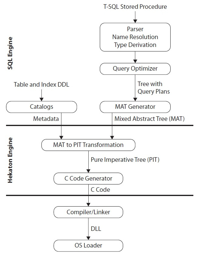
Figure 7.12 – Architecture of the Hekaton compiler

DLLs for both memory-optimized tables and natively compiled stored procedures are recompiled during recovery every time the SQL Server instance is started. SQL Server maintains the information that’s required to recreate these DLLs in each database metadata.

It is interesting to note that the generated DLLs are not kept in the database but in the filesystem. You can find them, along with some other intermediate files, by looking at the location that’s returned by the following query:

SELECT name, description FROM sys.dm_os_loaded_modules

where description = 'XTP Native DLL'

The following is a sample output:

A directory is created in the xtp directory that’s named after the database ID – in this case, 7. Next, the names of the DLL files start with xtp, followed by t for tables and p for stored procedures. Again, we have the database ID on the name (in this case, 7), followed by the object ID, which is 885578193 for the TransactionHistoryArchive table and 917578307 for the test natively compiled stored procedure.

Note

You may have noticed the name xtp several times in this chapter already. xtp stands for eXtreme Transaction Processing and was reportedly the original name of the feature before it was changed to in-memory OLTP.

You can inspect the listed directories and find the DLL file, the C source code, and several other files, as shown in the following screenshot:

Figure 7.13 – DLL and other files created during the compilation process

There is no need to maintain these files because SQL Server automatically removes them when they are no longer needed. If you drop both the table and procedure we just created, all these files will be automatically deleted by the garbage collector, although it may not happen immediately, especially for tables. Run the following statements to test this:

DROP PROCEDURE test

DROP TABLE TransactionHistoryArchive

Also, notice that you would need to delete the procedure first to avoid error 3729, as explained earlier.

Having those files on the filesystem does not represent a security risk (for example, in the case that they could be manually altered). Every time Hekaton has to load the DLLs again, such as when an instance is restarted or a database is put offline and then back online, SQL Server will compile the DLLs again, and those existing files are never used. That being said, let’s check out some of the limitations and enhancements that OLTP has.

Limitations and later enhancements

Without a doubt, the main limitation of the original release of Hekaton, SQL Server 2014, was that tables couldn’t be changed after being created: a new table with the required changes would have to be created instead. This was the case for any change you wanted to make to a table, such as adding a new column or index or changing the bucket count of a hash index. Creating a new table would require several other operations as well, such as copying its data to another location, dropping the table, creating the new table with the needed changes, and copying the data back, which would require some downtime for a production application. This limitation was probably the biggest challenge for deployed applications, which, of course, demanded serious thinking and architecture design to avoid or minimize changes once the required memory-optimized tables were in production.

In addition, dropping and creating a table would usually imply some other operations, such as scripting all its permissions. And because natively compiled stored procedures are schema bound, this also means that they need to be dropped first before the table can be dropped. That is, you need to script these procedures, drop them, and create them again once the new table is created. Similar to tables, you may need to script the permissions of the procedures as well. Updating statistics with the FULLSCAN option was also highly recommended after the table was created and all the data was loaded to help the query optimizer get the best possible execution plan.

You also weren’t able to alter natively compiled stored procedures on the original release, or even recompile them (except in a few limited cases, such as when the SQL Server instance was restarted or when a database was put offline and back online). As mentioned previously, to alter a native stored procedure, you would need to script the permissions, drop the procedure, create the new version of the procedure, and apply for the permissions again. This means that the procedure would not be available while you were performing those steps.

Starting with SQL Server 2016, the second in-memory OLTP release, the feature now includes the ability to change tables and native procedures by using the ALTER TABLE and ALTER PROCEDURE statements, respectively. This is a remarkable improvement after the initial release. However, some of the previously listed limitations remain. For example, although you can just use ALTER TABLE to change a table structure, SQL Server will still need to perform some operations in the background, such as copying its data to another location, dropping the table, creating the new table with the needed changes, and copying the data back, which would still require some downtime in the case of a production application. Because of this, you still need to carefully work on your original database design. There is no longer the need to script permissions for either tables or native store procedures when you use the ALTER TABLE and ALTER PROCEDURE statements.

Finally, there were some differences regarding statistics and recompiles in Hekaton compared to disk-based tables and traditional stored procedures on the original release. As the data in Hekaton tables changed, statistics were never automatically updated and you needed to manually update them by running the UPDATE STATISTICS statement with the FULLSCAN and NORECOMPUTE options. Also, even after your statistics are updated, existing natively compiled stored procedures cannot benefit from them automatically, and, as mentioned earlier, you cannot force a recompile either. You have to manually drop and recreate the native stored procedures.

Starting with SQL Server 2016, statistics used by the query optimizer are now automatically updated, as is the case for disk-based tables. You can also specify a sample when manually updating statistics as UPDATE STATISTICS with the FULLSCAN option was the only choice available in SQL Server 2014. However, updated statistics still do not immediately benefit native stored procedures in the same way as with traditional stored procedures. This means that a change in the statistics object will never trigger a new procedure optimization. So, you will still have to manually recompile a specific native stored procedure using sp_recompile, available only on SQL Server 2016 and later.

The original release of in-memory OLTP had serious limitations regarding memory as the total size for all the tables in a database could not exceed 256 GB. After the release of SQL Server 2016, this limit was originally extended to 2 TB, which was not a hard limit, just a supported limit. A few weeks after SQL Server 2016 was released, this new limit was also removed and Microsoft announced that memory-optimized tables could use any amount of memory available to the operating system.

Note

The documentation at https://docs.microsoft.com/en-us/sql/sql-server/what-s-new-in-sql-server-2016 still shows a supported limit of up to 2 TB, but https://techcommunity.microsoft.com/t5/sql-server-blog/increased-memory-size-for-in-memory-oltp-in-sql-server-2016/ba-p/384750 indicates that you can grow your memory-optimized tables as large as you like, so long as you have enough memory available.

The FOREIGN KEY, UNIQUE, and CHECK constraints were not supported in the initial release. They were supported starting with SQL Server 2016. Computed columns in memory-optimized tables and the CROSS APPLY operator on natively compiled modules are supported starting with SQL Server 2019.

The original release of in-memory OLTP required you to use a BIN2 collation when creating indexes on string columns, such as char, nchar, varchar, or nvarchar. In addition, comparing, sorting, and manipulating character strings that did not use a BIN2 collation was not supported with natively compiled stored procedures. Both restrictions have been lifted with SQL Server 2016 and now you can use any collation you wish.

Finally, you can use the following document to review all the SQL Server features that are not supported on a database that contains memory-optimized objects: https://docs.microsoft.com/en-us/sql/relational-databases/in-memory-oltp/unsupported-sql-server-features-for-in-memory-oltp. Hekaton tables and stored procedures do not support the full T-SQL surface area that is supported by disk-based tables and regular stored procedures. For an entire list of unsupported T-SQL constructs on Hekaton tables and stored procedures, see http://msdn.microsoft.com/en-us/library/dn246937(v=sql.120).aspx.

Summary

This chapter covered in-memory OLTP, originally known as Hekaton, which without a doubt was the most important new feature of SQL Server 2014. The Hekaton OLTP database engine is a response to a new design and architectural approach looking to achieve the most benefit of the new hardware available today. Although optimization for main memory access is its main feature and is even part of its name, Hekaton’s performance improvement is also complemented by other major architecture areas, such as compiling procedures to native code, as well as latches and lock elimination.

This chapter covered the Hekaton architecture and its main components – memory-optimized tables, hash, and range indexes, and natively compiled stored procedures were explained in great detail. Although Hekaton had several limitations in its first release in SQL Server 2014, multiple limitations have been lifted after four new releases, including SQL Server 2022.

xVelocity memory-optimized columnstore indexes, another in-memory technology, will be covered in Chapter 11, An Introduction to Data Warehouses. In the next chapter, we will learn more about plan caching.