
Cash Flow Forecasting
Abstract
This chapter describes by means of an example how a cash flow table can be produced from a critical path network and bar chart. Graphs can then be produced to show the cash flow and the relationship between the inflow and outflow curves.
Keywords
Cash flow; inflow curve; outflow curve
Chapter Outline
It has been stated in Chapter 30 that it is very easy to convert a network into a bar chart, especially if the durations and week (or day) numbers have been inserted. Indeed, the graphical method of analysis actually generates the bar chart as it is developed.
If we now divide this bar chart into a number of time periods (say, weeks or months) it is possible to see, by adding up vertically, what work has to be carried out in any time period. For example, if the time period is in months, then in any particular month we can see that one section is being excavated, another is being concreted, and another is being scaffolded and shuttered, etc.
From the description we can identify the work and can then find the appropriate rate (or total cost) from the bills of quantities. If the total period of that work takes six weeks and we have used up four weeks in the time period under consideration, then approximately two-thirds of the value of that operation has been performed and could be certificated.
By this process it is possible to build up a fairly accurate picture of anticipated expenditure at the beginning of the job, which in itself might well affect the whole tendering policy. Provided the job is on programme, the cash flow can be calculated, but, naturally, due allowance must be made for the different methods and periods of retentions, billing, and reimbursement. The cost of the operation must therefore be broken down into six main constituents:
By drawing up a table of the main operations as shown on the network, and splitting up the cost of these operations (or activities) into the six constituents, it is possible to calculate the average percentage that each constituent contains in relation to the value. It is very important, however, to deduct the values of the subcontracts from any operation and treat these subcontracts separately. The reason for this is, of course, that a subcontract is self-contained and is often of a specialized nature. To break up a subcontract into labour, plant, materials, etc., would not only be very difficult (since this is the prerogative of the subcontractor) but would also seriously distort the true distribution of the remainder of the project.
Example of Cash Flow Forecasting
The simplest way to explain the method is to work through the example described in Figures 31.1 to 31.6. This is a hypothetical construction project of three identical simple unheated warehouses with a steel framework on independent foundation blocks, profiled steel roof and side cladding, and a reinforced-concrete ground slab. It has been assumed that as an area of site has been cleared, excavation work can start, and the sequences of each warehouse are identical. The layout is shown in Figure 31.1 and the network for the three warehouses is shown in Figure 31.2.
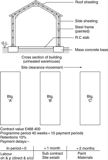

Figure 31.3 shows the graphical analysis of the network separated for each building. The floats can be easily seen by inspection, e.g., there is a two-week float in the first paint activity (58–59) since there is a gap between the following dummy 59–68 and activity 68–69. The speed and ease of this method soon become apparent after a little practice.

The bar chart in Figure 31.5 has been drawn straight from the network (Figure 31.2) and the costs in $100 units added from Figure 31.4. For example, in Figure 31.4 the value of foundation excavation for any one building is $9,400 per four-week activity. Since there are two four-week activities, the total is $18,800. To enable the activity to be costed in the corresponding measurement period, it is convenient to split this up into two-weekly periods of $4,700. Hence in Figure 31.5, foundation excavation for building A is shown as

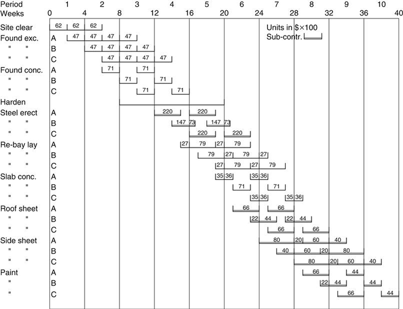
The summation of all the costs in any period is shown in Figure 31.6.

Figure 31.6 clearly shows the effect of the anticipated delays in payment of certificates and settlement of contractor’s accounts. For example, material valued at 118 in period 2 is paid to the contractor after one month in period 3 (part of the 331, which is 90% of 368, the total value of period 2), and is paid to the supplier by the contractor in period 4 after the two-month delay period.
From Figure 31.6 it can be seen that it has been decided to extract overhead and profit monthly as the job proceeds, but this is a policy that is not followed by every company. Similarly, the payment delays may differ in practice, but the principle would be the same.
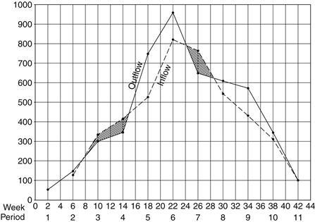
Figure 31.6 shows the total outflow and inflow for each time period and the net differences between the two. When these values are plotted on graphs as in Figures 31.7 and 31.8, it can be seen that there are only three periods of positive cash flow, i.e., periods 3, 4, and 7. However, while this shows the actual periods when additional moneys have to be made available to fund the project, it does not show, because the gap between the outflow and inflow is so large for most of the time, that for all intents and purposes the project has a negative cash flow throughout its life.

This becomes apparent when the cumulative outflows and inflows, which are tabulated in the last three lines of Figure 31.6, are plotted on a graph as in Figure 31.9 and 31.10. From these it can be seen that cumulatively, the Chapter_27 13.01.38 13.01.38 13.01.38 13.01.38.pages a positive cash flow (a mere $500) is in period 4.
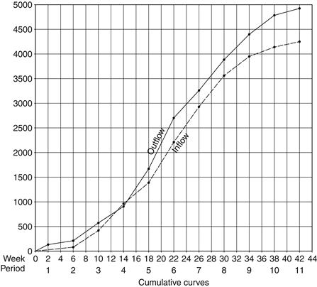
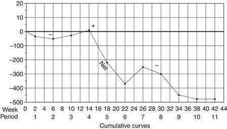
Figure 31.10
This example shows that the project is not self-financing and will possibly only show a profit when the 10% retention moneys have been released. To restore the project to a positive cash flow, it would be necessary to negotiate a sufficiently large mobilization fee at the start of the project to ensure that the contract is self-financing.