
Cost Control and EVA
Abstract
Thia chapter describes the principles of earned value analysis (EVA) and the very similar Foster Wheeler SMAC manhour control system. The advantages of EVA over the traditional weighting system are discussed together with an example showing how to recalculate the earned value and final forecast after poor progress due to re-work. Formulae are provided for calculating earned value, overall % completion, efficiency, and final forecast in either manhours or cost. The chapter also includes a section on EVA in civil engineering and the integration of materials with EVA.
Keywords
Earned value analysis; EVA; % complete; actual hours; value hours; budget hours; forecast final hours; integration of materials; SMAC
Chapter Outline
Apart from ensuring that their project is completed on time, all managers, whether in the office, workshop, factory, or on-site, are concerned with cost. There is little consolation in finishing on time, when, from a cost point of view, one wished the job had never started!
Cost control has been a vital function of management since the days of the pyramids, but only too frequently is the term confused with mere cost reporting. The cost report is usually part of every manager’s monthly report to his superiors, but an account of the past month’s expenditure is only stating historical facts. What the manager needs is a regular and up-to-date monitoring system that enables him to identify the expenditure with specific operations or stages, determine whether the expenditure was cost-effective, plot or calculate the trend, and then take immediate action if the trend is unacceptable.
Network analysis forms an excellent base for any cost-control system, since the activities can each be identified and costed, so that the percentage completion of an activity can also give the proportion of expenditure, if that expenditure is time related. The system is ideal, therefore, for construction sites, drawing offices, or factories where the basic unit of control is the manhour.
SMAC – Manhour Control
Site manhours and cost (SMAC)∗ is a cost control system developed in 1978 specifically on a critical path network base for either manual or computerized cost and progress monitoring, which enables performance to be measured and trends to be evaluated, thus providing the project manager with an effective instrument for further action. The system, which is now known as earned value analysis (EVA), can be used for all operations where manhours or costs have to be controlled, and since most functions in an industrial (and now more and more commercial) environment are based on manhours and can be planned with critical path networks, the utilization of the system is almost limitless.
The following operations or activities could benefit from the system:
The criteria laid down when the system was first mooted were:
1. Minimum site (or workshop) input. Site staff should spend their time managing the contract and not filling in unnecessary forms.
2. Speed. The returns should be monitored and analysed quickly so that action can be taken.
3. Accuracy. The manhour expenditure must be identifiable with specific activities that are naturally logged on time sheets.
4. Value for money. The useful manhours on an activity must be comparable with the actual hours expended.
5. Economy. The system must be inexpensive to operate.
6. Forward looking. Trends must be seen quickly so that remedial action can be taken when necessary.
The final system satisfied all these criteria with the additional advantage that the percentage complete returns become a simple but effective feedback for updating the network programme.
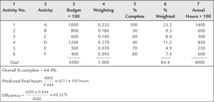
One of the most significant differences between EVA and the conventional progress-reporting systems is the substitution of ‘weightings’ given to individual activities, by the concept of ‘value hours’. If each activity is monitored against its budget hours (or the hours allocated at the beginning of the contract, to that activity) then the ‘value hour’ is simply the percentage complete of that activity multiplied by its budget hours. In other words, it is the useful hours against the actual hours recorded on the time sheets.
If all the value hours of a project are added up and the total divided by the total budget hours, the overall per cent complete of the project is immediately seen.
The advantage of this system over the weighting system is that activities can be added or eliminated without having to ‘re-weight’ all the other activities. Furthermore, the value hours are a tangible parameter, which, if plotted on a graph against actual hours, budget hours, and predicted final hours, gives the manager a ‘feel’ of the progress of the job that is second to none. The examples in Table 32.1 and 32.2 show the difference between the two systems.

Summary of Advantages
Comparing the weighting and value hours systems, the following advantages of the value hours system are immediately apparent:
1. The basic value hours system requires only six columns against the weighting system’s seven.
2. There is no need to carry out a preliminary time-consuming ‘weighting’ at the beginning of the job.
3. Activities can be added or removed or have the durations changed without the need to recalculate the weightings of each activity. This saves hundreds of manhours on a large project.
4. The value hours are easily calculated and can even, in many cases, be assessed by inspection.
5. Errors are easily seen, as the value can never be more than the budget.
6. Budget hours, actual hours, value hours, and forecast hours can all be plotted on one graph to show trends.
7. The method is ideal for assessing the value of work actually completed for progress payments to main and subcontractors. Since it is based on manhours, it truly represents construction progress independently of material or plant costs, which so often distort the assessment.
The efficiency (output/input) for each activity is obtained by dividing the value hours by the actual hours. This is also known as the cost performance index (CPI).
The analysis can be considerably enhanced by calculating the efficiency and forecast final hours for each activity and adding these to the table.
The forecast final hours are obtained by either:
Both these methods give the same answer as the following proof (using the same abbreviations) shows:
(a) Final hours = ![]()
Efficiency (CPI) = ![]() (value is always the numerator)
(value is always the numerator)
Hence, Final hours = ![]()
But Value = Budget × % complete = B × D
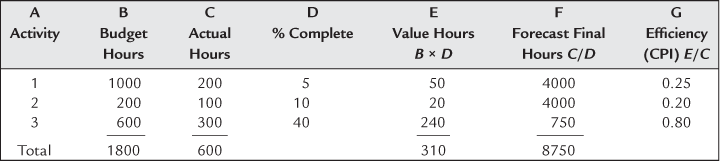
Example 1 shows the earned value table for a small project consisting of three activities where there was reasonable progress.

The overall percentage complete of the work can be obtained by adding all the value hours in column E and dividing them by the total budget hours in column B, i.e., E/B.
It can be seen that the difference between the calculated final hours of 2000, and the sum of the values of column F of 1950, is only 50 hours or 2.5%, and this tends to be the variation on projects with a large number of activities.
When an analysis is carried out after a period of poor progress as shown in the table of Example 2, the increase in the forecast final hours and the decrease in the efficiency become immediately apparent. An examination of the table shows that this is due to the abysmal efficiencies (column G) of activities 1 and 2.
In this example the overall % complete is:

This is still a large overrun, but it is considerably less than the massive 8750 hours produced by adding up the individual forecast final hours in column F.
Clearly such a discrepancy of 5266 hours in Example 2 calls for an examination. The answer lies in the offending activities 1 and 2, which need to be restated so that the actual hours reflect the actual situation on the job. For example, if it is found that activities 1 and 2 required rework to such an extent that the original work was completely wasted and the job had to be started again, it is sensible to restate the actual hours of these activities to reflect this, i.e., all the abortive work is ‘written off’ and a new assessment of 0% complete is made from the starting point of the rework. There is little virtue in handicapping the final forecast with the gross inefficiency caused by an unforeseen rework problems. Such a restatement is shown in Example 2a.

Comparing Examples 2 and 2a it will be noted that:
1. The total budget hours are the same, i.e., 1800;
2. The total actual hours are now only 350 in 2a because 180 hours have been written off for activity 1A and 70 hours have been written off for activity 2A;
3. The value hours are the same, i.e., 310;
4. The overall % complete is the same;
5. The forecast final hours are now only 1700 because although the 250 aborted hours had to be included, the efficiency of the revised activities 1B and 2B has improved;
The forecast final hours calculated by dividing the budget hours by the efficiency comes to 1800/0.885 = 2033 hours. This is more than the 1700 hours obtained by adding all the values in column F, but the difference is only because the percentage complete assessment of activities is so diverse.
In practice, such a difference is both common and acceptable because:
1. On medium or large projects, wide variations of % complete assessments tend to follow the law of ‘swings and roundabouts’ and cancel each other out.
2. In most cases therefore the sensible method of forecasting the final hours is to either:
(a) divide the budget hours by the efficiency, i.e., B/G or
(b) divide the actual hours by the % complete, i.e., C/D. Both of course, give the same answer.
3. The column F (forecast final hours) is in most cases not required, but should it be necessary to find the forecast final hours of a specific activity, this can be done at any stage by simply dividing the actual hours of that activity by its percentage complete.
4. It must be remembered that comparing the forecast final hours with the original budget hours is only a reporting function and its use should not be given too much emphasis. A much more important comparison is that between the actual hours and the value hours as this is a powerful and essential control function.
As stated earlier, two of the criteria of the system were the absolute minimum amount of form filling for reporting progress and the accurate assessment of percentage complete of specific activities. The first requirement is met by cutting down the reporting items to three essentials:
1. The activity numbers of the activities worked on in the reporting period (usually one week).
2. The actual hours spent on each of these activities, taken from the time cards.
3. The assessment of the percentage complete of each reported activity. This is made by the ‘man on the spot’.
The third item is the most likely one to be inaccurate, since any estimate is a mixture of fact and opinion. To reduce this risk (and thus comply with the second criterion, i.e., accuracy) the activities on the network have to be chosen and ‘sized’ to enable them to be estimated, measured, or assessed in the field, shop, or office by the foreman or supervisor in charge. This is an absolute prerequisite of success, and its importance cannot be over-emphasized.
Individual activities must not be so complex or long (in time) that further breakdown is necessary in the field, nor should they be so small as to cause unnecessary paperwork. For example, the erection of a length of ducting and supports (Figure 32.1) could be split into the activities shown in Figure 32.2 and 32.3.


Figure 32.2

Figure 32.3
Any competent supervisor can see that if the two columns of frame 1 (Activity 1) have been erected and stayed, the activity is about 50% complete. He may be conservative and report 40% or optimistic and report 60%, but this ±20% difference is not important in the light of the total project. When all these individual estimates are summated the discrepancies tend to cancel out. What is important is that the assessment is realistic and checkable. Similarly, if 3 m of the duct between frames 1 and 2 have been erected, it is about 30% complete. Again, a margin on each side of this estimate is permissible.
However, if the network were prepared as shown in Figure 32.3 the supervisor may have some difficulty in assessing the percentage complete of activity 1 when he had erected and stayed the columns of frame 1. He now has to mentally compute the manhours to erect and stay two columns in relation to four columns and four beams. The percentage complete could be between 10% and 30%, with an average of 20%. The ± percentage difference is now 50%, which is more than double the difference in the first network. It can be seen therefore that the possibility of error and the amount of effort to make an assessment or both is greater.
Had the size of each activity been reduced to each column, beam, or brace, the clerical effort would have been increased and the whole exercise would have been less viable. It is important therefore to consult the men in the field or on the shop floor before drafting the network and fixing the sequence and duration of each activity.
EVA for Civil Engineering Projects
Most civil engineering contracts have an in-built earned value system, because the monthly re-measure is in fact a valuation of the work done. By using the composite rates in the bill of quantities or the schedule of rates, the monetary value of the work done to date can be easily established. This can then be translated into a curve and the value at any time period can then be divided by the corresponding value of the cash flow curve (which is in effect the planned work) to give the approximate % complete (SPI). However these values do not give a true picture of the work actually done, as the rates in the bills include overheads and profit as well as contingency allowance.
In order to compare Actual Costs with Earned Value, it is necessary therefore to take the contingency, profit, and overhead portion out of the unit rates so that only true labour, material, and plant costs remain. This reduction could be between 5% and 10%. Re-measuring of the completed work can then take place as normal in the conventional physical units of m. m2, m3, tonne, etc. The measured quantities are then multiplied by the new (reduced) rates to give the useful work done in monetary terms and become in effect the Earned Value.
Planned costs
These cab be taken from the “S” curve of the histogram or cash flow curve. These will include labour, materials and plant costs, but they must again be at the reduced rate. i.e. without overheads and profit)

Site Overheads
Establishment costs and indirect labour costs cannot be part of the EVA system. However, the must be recorded separately. The indirect labour costs must be plotted on the bottom of the EVA set of curves to ensure that they have not been inflated to off-set overruns of direct labour costs.
As with the normal EVA system, at any particular point in time,
| Earned Value (EV) | = Measured work in ≤, $, Euros etc. |
| Overall % complete | = EV / total original budget |
| Efficiency (CPI) | = EV / Actual Costs |
| SPI | = EV / Planned Costs |
Where there are no Bills of Quantities, labour costs can still be used for monitoring progress using the EVA system. Material and plant costs can never be used for monitoring progress.
To operate such an EVA system, the budget costs, planned costs and actual costs (and the calculated earned value) must must be broken down into labour, materials and plant for each activity, as each is measured differently. For any particular point in time, it is quite possible to have installed the planned materials materials and expended the associated plant costs and yet have an overrun or under run of labour costs, depending on the effectiveness of supervision, method of working, climatic conditions or a myriad of other factors.
It can be seen therefore, that this breakdown of each activity into three cost items can be very time consuming and for this reason the conventional monthly measurement of completed work based on on the rates in the Bills of Quantities, is the preferred method used by most companies in the civil engineering and building industries.”
In case of any queries to this correction, I have attached a word document with how it should look.
Example
A large storage tank consisting of 400 steel plates, which at $150 each, gives a material cost of $60000 (for simplicity, other material costs have been ignored).
The duration for erecting and testing is six weeks.
The labour (mostly welding) manhours are 1200, which at $20/hour, gives a labour cost of $24000.
Again, for simplicity, plant costs (cranes and welding sets) are regarded as site overheads and can be ignored.
All the plates arrive on site on day 1 and have to be paid for at day 28.
Work starts as soon as the plates have been unloaded (by others).
By day 7 (1 week later) 60 plates have been erected and welded.
Therefore at day 7, the percentage complete is 60/400 = 15%.
The EV calculations are carried out weekly and the time sheets show that after the first week, the men have booked a total of 200 manhours.
The earned value is therefore 15% of 1200 = 180, so that the efficiency (CPI) = 180/200 = 90%.
If the men are paid production bonuses, they would not get a bonus for this week as the productivity bonus (as agreed with the unions) only starts at 97% efficiency.
The costs incurred to date are therefore only labour costs and are 200 × $20 = $4000.
At day 28 (after 4 weeks) 300 plates have been erected.
The % complete is now 300/400 = 75%.
The total manhours booked to date are now 850.
The earned value can be seen to be 75% of 1200 = 900.
As the efficiency (CPI) is now 900/850 = 105%, the men get their bonus.
The cost to date is now 850 × $20 = $17000 plus the total material cost of $60000 = $77000.
Note that all the material has to be paid for – not just the material erected.
Alternative Payment Schedule
Supposing the terms of the contract were that the tank contractor had to be paid weekly for material and labour. He would therefore be paid as follows:
At the end of week 1:
Labour: 180 manhours = $3600 (the earned value, not the actual cost)
Material: 60 plates at $150/plate = 150 × 60 = $9000 (the plates erected)
The total payment is therefore $3600 + 9000 = $12600 (ignoring retentions).
It can be seen therefore that materials can be a useful aid in assessing percentage complete, and although in order to obtain the total costs, they must be added to the labour costs, they cannot be part of the EV analysis. In other words, with the exception of the individual percentage complete assessment, the earned value, CPI, SPI, anticipated final cost, and anticipated final completion time can only be calculated from the labour data.
The types of work that lend themselves to a similar treatment as the storage tank are:
• Cable runs measured in metres
• Insulation measured in metres or sq. metres
• Steelwork measured in tonnes
All labour must of course be measured in manhours or money units.
If plant costs have to be booked to the work package, they can be treated in a similar way to equipment, except that payments (when the plant is hired) are usually made monthly.
∗SMAC is the proprietary name given to the cost-control program developed by Foster Wheeler.