
Basic Network Principles
Abstract
This chapter explains in detail the principles of network analysis and the way networks are produced from simple logic diagrams to full construction networks.
The differences between and advantages and disadvantages of activity on arrow (AoN) and activity on node (AoN) diagrams are discussed. The use of hammocks and ladders and the different network configurations or constraints are described. The last part of the chapter discusses the use of bar charts (or Gantt charts) and time scale networks.
Keywords
Network diagram; critical path diagram; activity on arrow (AoN); activity on node (AoN); durations; nodes; hammocks; ladders; network configuration; numbering; coordinate; grid; bar chart; Gantt chart; constraints
Chapter Outline
It is true to say that whenever a process requires a large number of separate but integrated operations, a critical path network can be used to advantage. This does not mean, of course, that other methods are not successful or that the critical path method (CPM) is a substitute for these methods – indeed, in many cases network analysis can be used in conjunction with traditional techniques – but if correctly applied CPM will give a clearer picture of the complete programme than other systems evolved to date.
Every time we do anything, we string together, knowingly or unknowingly, a series of activities that make up the operation we are performing. Again, if we so desire, we can break down each individual activity into further components until we end up with the movement of an electron around a nucleus. Clearly, it is ludicrous to go to such a limit but we can call a halt to this successive breakdown at any stage to suit our requirements. The degree of the breakdown depends on the operation we are performing or intend to perform.
In the UK it was the construction industry that first realized the potential of network analysis, and most of, if not all, the large construction, civil engineering, and building firms now use CPM regularly for their larger contracts. However, a contract does not have to be large before CPM can be usefully employed. If any process can be split into twenty or more operations or ‘activities’, a network will show their interrelationship in a clear and logical manner so that it may be possible to plan and rearrange these interrelationships to produce either a shorter or a cheaper project, or both.
Network Analysis
Network analysis, as the name implies, consists of two basic operations:
The Network
Basically the network is a flow diagram showing the sequence of operations of a process. Each individual operation is known as an activity and each meeting point or transfer stage between one activity and another is an event or node. If the activities are represented by straight lines and the events by circles, it is very simple to draw their relationships graphically, and the resulting diagram is known as the network. In order to show whether an activity has to be performed before or after its neighbour, arrowheads are placed on the straight lines, but it must be explained that the length or orientation of these lines is quite arbitrary. This format of network is called activity on arrow (AoA), as the activity description is written over the arrow.
It can be seen, therefore, that each activity has two nodes or events; one at the beginning and one at the end (Figure 19.1). Thus events 1 and 2 in the figure show the start and finish of activity A. The arrowhead indicates that 1 comes before 2, i.e., the operation flows towards 2.
![]()
Figure 19.1
We can now describe the activity in two ways:
For analysis purposes (except when using a computer), the second method must be used.
Basic Rules
Before proceeding further it may be prudent at this stage to list some very simple but basic rules for network presentation, which must be adhered to rigidly:
1. Where the starting node of an activity is also the finishing node of one or more other activities, it means that all the activities with this finishing node must be completed before the activity starting from that node can be commenced. For example, in Figure 19.2, 1–3(A) and 2–3(B) must be completed before 3–4(C) can be started.

Figure 19.2
2. Each activity must have a different set of starting and finishing node numbers. This poses a problem when two activities start and finish at the same event node, and means that the example shown in Figure 19.3 is incorrect. In order to apply this rule, therefore, an artificial or ‘dummy’ activity is introduced into the network (Figure 19.4). This ‘dummy’ has a duration of zero time and thus does not affect the logic or overall time of the project. It can be seen that activity A still starts at 1 and takes 7 units of time before being completed at event 3. Activity B also still takes 7 units of time before being completed at 3, but it starts at node 2. The activity between 1 and 2 is a timeless dummy.

Figure 19.3

Figure 19.4
3. When two chains of activities are interrelated, this can be shown by joining the two chains either by a linking activity or a ‘dummy’ (Figure 19.5). The dummy’s function is to show that all the activities preceding it, i.e., 1–2(A) and 2–3(B) shown in Figure 20.5, must be completed before activity 7–8(F) can be started. Needless to say, activities 5–6(D), 6–7(E), and 2–6(G) must also be completed before 7–8(F) can be started.

Figure 19.5
4. Each activity (except the last) must run into another activity. Failure to do so creates a loose end or ‘dangle’ (Figure 19.6). Dangles create premature ‘ends’ of a part of a project, so that the relationship between this end and the actual final completion node cannot be seen. Hence the loose ends must be joined to the final node (in this case, node 6 in Figure 19.7) to enable the analysis to be completed.

Figure 19.6

Figure 19.7
5. No chain of activities must be permitted to form a loop, i.e., such a sequence that the last activity in the chain has an influence on the first. Clearly, such a loop makes nonsense of any logic since, if one considers activities 2–3(B), 3–4(C), 4–5(E), and 5–2(F) in Figure 19.8, one finds that B, C, and E must precede F, yet F must be completed before B can start. Such a situation cannot occur in nature and defies analysis.
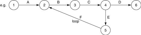
Figure 19.8
Apart from strictly following the basic rules 1 to 5 set out above, the following points are worth remembering to obtain the maximum benefit from network techniques.
1. Maximize the number of activities that can be carried out in parallel. This obviously (resources permitting) cuts down the overall programme time.
2. Beware of imposing unnecessary restraints on any activity. If a restraint is convenient rather than imperative, it should best be omitted. The use of resource restraints is a trap to be particularly avoided since additional resources can often be mustered – even if at additional cost. The exception is when using ‘critical chain’ project management methods.
3. Start activities as early as possible and connect them to the rest of the network as late as possible (Figures 19.9 and 19.10). This avoids unnecessary restraints and gives maximum float.
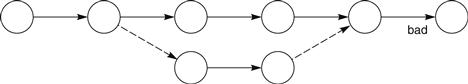
Figure 19.9
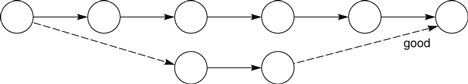
Figure 19.10
4. Resist the temptation to use a conveniently close node point as a ‘staging post’ for a dummy activity used as a restraint. Such a break in a restraint could impose an additional unnecessary restraint on the succeeding activity. In Figure 19.11 the intent is to restrain activity E by B and D and activity G by D. However, because the dummy from B uses node 6 as a staging post, activity G is also restrained by B. The correct network is shown in Figure 19.12. It must be remembered that the restraint on G may have to be added at a later stage, so that the effect of B in Figure 19.11 may well be overlooked.

Figure 19.11
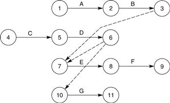
Figure 19.12
5. When drawing ladder networks beware of the danger of trying to economize on dummy activities as described later (Figures 19.24 and 19.25).
Durations
Having drawn the network in accordance with the logical sequence of the particular project requirements, the next step is to ascertain the duration or time of each activity. These may be estimated in the light of experience, in the same manner that any programme times are usually ascertained, e.g., using standard industry or company norms, but it must be remembered that the shorter the durations, the more accurate they usually are.
The durations are then written against each activity in any convenient time unit, but this must, of course, be the same for every activity. For example, referring to Figure 19.13, if activities 1–2(A), 2–5(B), and 5–6(C) took 3, 2, and 7 days, respectively, one would show this by merely writing these times under the activity.
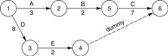
Figure 19.13
Numbering
The next stage of network preparation is numbering the events or nodes. Depending on the method of analysis, the following systems shown in Figure 19.14 can be used.
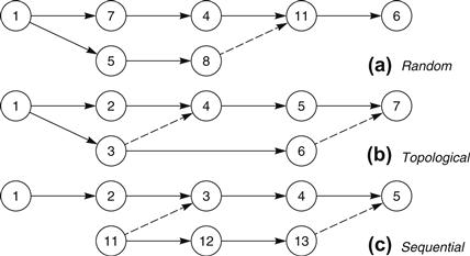
Figure 19.14
Random
This method, as the name implies, follows no pattern and merely requires each node number to be different. All computers (if used) can, of course, accept this numbering system, but there is always the danger that a number may be repeated.
Topological
This method was necessary for the original early computer programs, which demanded that the starting node of an activity be smaller than the finishing node of that activity. If this law is applied throughout the network, the node numbers will increase in value as the project moves towards the final activity. It had some value for beginners using network analysis since loops are automatically avoided. However, it is very time consuming and requires constant back-checking to ensure that no activity has been missed. The real drawback is that if an activity is added or changed, the whole network has to be renumbered from that point onwards. Clearly, this is an unacceptable restriction in practice and, with the development of modern computer programs, can now be consigned to the history books of project planning.
Sequential
This is a random system from an analysis point of view, but the numbers are chosen in blocks so that certain types of activities can be identified by the nodes. The system therefore clarifies activities and facilitates recognition. The method is quick and easy to use, and should always be used whatever method of analysis is employed. Sequential numbering is usually employed when the network is banded (see Chapter 20). It is useful in such circumstances to start the node numbers in each band with the same prefix number, i.e., the nodes in band 1 would be numbered 101, 102, 103, etc., while the nodes in band 2 are numbered 201, 202, 203, etc. Figure 20.1 would lend itself to this type of numbering.
Coordinates
This method of activity identification can only be used if the network is drawn on a gridded background. In practice, thin lines are first drawn on the back of the translucent sheet of drawing paper to form a grid. This grid is then given coordinates or map references with letters for the vertical coordinate and numbers for the horizontal (Figure 19.15).
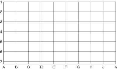
The reason for drawing the lines on the back of the paper is, of course, to leave the grid intact when the activities are changed or erased. A fully drawn grid may be confusing to some people, so it may be preferable to draw a grid showing the intersections only (Figure 19.16).

When activities are drawn, they are confined in length to the distance between two intersections. The node is drawn on the actual intersection so that the coordinates of the intersection become the node number. The number may be written in or the node left blank, as the analyst prefers.
As an alternative to writing the grid letters on the nodes, it may be advantageous to write the letters between the nodes as in Figure 23.3. This is more fully described in Chapter 23.
Figure 19.17 shows a section of a network drawn on a gridded background representing the early stages of a design project. As can be seen, there is no need to fill in the nodes, although, for clarity, activities A1–B1, B1–B2, A3–B3, A3–B4, and A5–C5 have had the node numbers added. The node numbers for ‘electrical layout’ would be B4–C4, and the map reference principle helps to find the activity on the network when discussing the programme on the telephone or quoting it in e-mail.
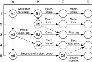
Figure 19.17
There is no need to restrict an activity to the distance between two adjacent intersections of coordinates. For example, A5–C5 takes up two spaces. Similarly, any space can also be used as a dummy and there is no restriction on the length or direction of dummies. It is, however, preferable to restrict activities to horizontal lines for ease of writing and subsequent identification.
When required, additional activities can always be inserted in an emergency by using suffix letters. For example, if activity ‘preliminary foundation drawings’ A3–B3 had to be preceded by, say, ‘obtain loads’, the network could be redrawn as shown in Figure 19.18.

Figure 19.18
Identifying or finding activities quickly on a network can be of great benefit, and the above method has considerable advantages over other numbering systems. The use of coordinates is particularly useful in minimizing the risk of duplicating node numbers in a large network. Since each node is, as it were, prenumbered by its coordinates, the possibility of double numbering is virtually eliminated.
Unfortunately, on the earlier computer programs, if the planner entered any number twice, the results could be disastrous, since the machine will, in many instances, interpret the error as a logical sequence. The following example shows how this is possible. The intended sequence is shown in Figure 19.19. If the planner by mistake enters a number 11 instead of 15 for the last event of activity d, the sequence will, in effect, be as shown in Figure 19.20, but the computer will interpret the error as in Figure 19.21. Clearly, this will give a wrong analysis. If this little network had been drawn on a grid with coordinates as node numbers, it would have appeared as in Figure 19.22. Since the planner knows that all activities on line B must start with a B, the chance of the error occurring is considerably reduced.
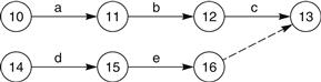
Figure 19.19
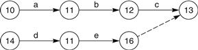
Figure 19.20
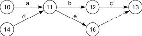
Figure 19.21

Figure 19.22
Hammocks
When a number of activities are in series, they can be summarized into one activity encompassing them all. Such a summary activity is called a hammock. It is assumed that only the first activity is dependent on another activity outside the hammock and only the last activity affects another activity outside the hammock.
On bar charts, hammocks are frequently shown as summary bars above the constituent activities and can therefore simplify the reporting document for a higher management who are generally not concerned with too much detail. For example, in Figure 19.22, activities A1 to A4 could be written as one hammock activity since only A1 and A4 are affected by work outside this activity string.
Ladders
When a string of activities repeats itself, the set of strings can be represented by a configuration known as a ladder. For a string consisting of, say, four activities relating to two stages of excavation, the configuration is shown in Figure 19.23.

Figure 19.23
This pattern indicates that, for example, hand trim of Stage II can only be done if
This, of course, is what it should be.
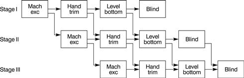
However, if the work were to be divided into three stages, the ladder could, on the face of it, be drawn as shown in Figure 19.24.

Figure 19.24
Again, in Stage II all the operations are shown logically in the correct sequence, but closer examination of Stage III operations will throw up a number of logic errors the inexperienced planner may miss.
What we are trying to show in the network is that Stage III hand trim cannot be performed until Stage III machine excavation is complete and Stage II hand trim is complete. However, what the diagram says is that, in addition to these restraints, Stage III hand trim cannot be performed until Stage I level bottom is also complete.
Clearly, this is an unnecessary restraint and cannot be tolerated. The correct way of drawing a ladder therefore when more than two stages are involved is as in Figure 19.25.

Figure 19.25
We must, in fact, introduce a dummy activity in Stage II (and any intermediate stages) between the starting and completion node of every activity except the last. In this way, the Stage III activities will not be restrained by Stage I activities except by those of the same type.
An examination of Figure 19.26 shows a new dummy between the activities in Stage II, i.e.
![]()
Figure 19.26
This concept led to the development of a new type of network presentation called the ‘Lester’ diagram, which is described more fully in Chapter 23. This has considerable advantages over the conventional arrow diagram and the precedence diagram, also described later.
Precedence or Activity on Node (AoN) Diagrams
Some planners prefer to show the interrelationship of activities by using the node as the activity box and interlinking them by lines. The durations are written in the activity box or node and are therefore called activity on node (AoN) diagrams. This has the advantage that separate dummy activities are eliminated. In a sense, each connecting line is, of course, a dummy because it is timeless. The network produced in this manner is also called variously a precedence diagram or a circle and link diagram. Precedence diagrams have a number of advantages over arrow (AoA) diagrams in that
2. They may be easier to understand by people familiar with flowsheets;
3. Activities are identified by one number instead of two so that a new activity can be inserted between two existing activities without changing the identifying node numbers of the existing activities; and
4. Overlapping activities can be shown very easily without the need for the extra dummies shown in Figure 19.25.
Analysis and float calculation (see Chapter 21) is identical to the methods employed for arrow diagrams and, if the box is large enough, the earliest and latest start and finishing times can be written.
A typical precedence network is shown in Figure 19.27 where the letters in the box represent the description or activity numbers. Durations are shown above-centre and the earliest and latest starting and finish times are given in the corners of the box, as explained in the key diagram. The top line of the activity box gives the earliest start (ES), duration (D), and earliest finish (EF).

Therefore:
![]()
The bottom line gives the latest start and the latest finish. Therefore:
![]()
The centre box is used to show the total float.
ES is, of course, the highest EF of the previous activities leading into it, i.e., the ES of activity E is 8, taken from the EF of activity B.
LF is the lowest LS of the previous activity working backwards, i.e., the LF of A is 3, taken from the LS of activity B.
The ES of activity F is 5 because it can start after activity D is 50% complete, i.e.,
Sometimes it is advantageous to add a percentage line on the bottom of the activity box to show the stage of completion before the next activity can start (Figure 19.28). Each vertical line represents 10% completion. Apart from showing when the next activity starts, the percentage line can also be used to indicate the percentage completion of the activity as a statement of progress once work has started, as in Figure 19.29.

Figure 19.28

There are two other advantages of the precedence diagram over the arrow diagram.
1. The risk of making the logic errors is virtually eliminated. This is because each activity is separated by a link, so that the unintended dependency from another activity is just not possible.
This is made clear by referring to Figure 19.30, which is the precedence representation of Figure 19.25.
As can be seen, there is no way for an activity like ‘Level bottom’ in Stage I to affect activity ‘Hand trim’ in Stage III, as is the case in Figure 19.30.
2. In a precedence diagram all the important information of an activity is shown in a neat box.
A close inspection of the precedence diagram (Figure 19.31) shows that in order to calculate the total float, it is necessary to carry out the forward and backward pass. Once this has been done, the total float of any activity is simply the difference between the latest finishing time (LF) obtained from the backward pass and the earliest finishing time (EF) obtained from the forward pass.

On the other hand, the free float can be calculated from the forward pass only, because it is simply the difference of the earliest start (ES) of a subsequent activity and the earliest finishing time (EF) of the activity in question.
This is clearly shown in Figure 19.31.
Despite the above-mentioned advantages, which are especially appreciated by people familiar with flow diagrams as used in manufacturing industries, many prefer the arrow diagram because it resembles more closely a bar chart. Although the arrows are not drawn to scale, they do represent a forward-moving operation and, by thickening up the actual line in approximately the same proportion as the reported progress, a ‘feel’ for the state of the job is immediately apparent.
One major disadvantage of precedence diagrams is the practical one of the size of the box. The box has to be large enough to show the activity title, duration, and earliest and latest times, so that the space taken up on a sheet of paper reduces the network size. By contrast, an arrow diagram is very economical, since the arrow is a natural line over which a title can be written and the node need be no larger than a few millimetres in diameter – if the coordinate method is used.
The difference (or similarity) between an arrow diagram and a precedence network is most easily seen by comparing the two methods in the following example. Figure 19.32 shows a project programme in AoA format and Figure 19.33 the same programme as a precedence diagram, or AoN format. The difference in area of paper required by the two methods is obvious (see also Chapter 33).


Figure 19.33 shows the precedence version of Figure 19.32.
In practice, the only information necessary when drafting the original network is the activity title, the duration, and, of course, the interrelationships of the activities. A precedence diagram can therefore be modified by drawing ellipses just big enough to contain the activity title and duration, leaving the computer (if used) to supply the other information at a later stage. The important thing is to establish an acceptable logic before the end date and the activity floats are computed. In explaining the principles of network diagrams in textbooks (and in examinations), letters are often used as activity titles, but in practice when building up a network, the real descriptions have to be used.
An example of such a diagram is shown in Figure 19.34. Care must be taken not to cross the nodes with the links and to insert the arrowheads to ensure the correct relationship.

One problem of a precedence diagram is that when large networks are being developed by a project team, the drafting of the boxes takes up a lot of time and paper space and the insertion of links (or dummy activities) becomes a nightmare, because it is confusing to cross the boxes, which are in effect nodes. It is necessary therefore to restrict the links to run horizontally or vertically between the boxes, which can lead to congestion of the lines, making the tracing of links very difficult.
When a large precedence network is drawn by a computer, the problem becomes even greater, because the link lines can sometimes be so close together that they will appear as one thick black line. This makes it impossible to determine the beginning or end of a link, thus nullifying the whole purpose of a network, i.e., to show the interrelationship and dependencies of the activities. (See Figure 19.35.)

For small networks with few dependencies, precedence diagrams are no problem, but for networks with 200–400 activities per page, it is a different matter. The planner must not feel restricted by the drafting limitations to develop an acceptable logic, and the tendency by some irresponsible software companies to advocate eliminating the manual drafting of a network altogether must be condemned. This manual process is after all the key operation for developing the project network and the distillation of the various ideas and inputs of the team. In other words, it is the thinking part of network analysis. The number crunching can then be left to the computer.
Once the network has been numbered and the times or durations added, it must be analyzed. This means that the earliest starting and completion dates must be ascertained and the floats or ‘spare times’ calculated. There are three main types of analysis:
Since these three different methods (although obviously giving the same answers) require very different approaches, a separate chapter has been devoted to each technique (see Chapters 21, 22, and 24).
Constraints
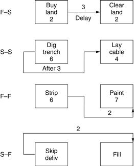
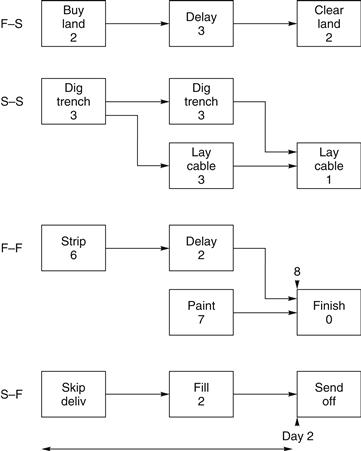
By far the most common logical constraint of a network is as given in the examples on the previous pages, i.e., ‘Finish to Start’ (F-S) where activity B can only start when activity A is complete. However, it is possible to configure other restraints. These are: Start to Start (S-S), Finish to Finish (F-F), and Start to Finish (S-F). Figure 19.36 shows these less usual constraints, which are sometimes used when a lag occurs between the activities. Analysing a network manually with such restraints can be very confusing, and should there be a lag or delay between any two activities, it is better to show this delay as just another activity. In fact all these three less usual constraints can be redrawn in the more conventional Finish to Start (F-S) mode as shown in Figure 19.37.
When an activity can start before the previous one has been completed, i.e., when there is an overlap, it is known as lead. When an activity cannot start until part of the previous activity has been completed, it is called a lag.
Bar (Gantt) Charts
The bar chart was originally first invented by a Polish engineer, Karol Adamiecki, but it was an American production engineer, Henry Laurence Gantt, who developed it at the beginning of the 20th century, and the chart is consequently known now as the Gantt chart. The Gantt chart was used in a number of planning applications during the first world war and was the main planning tool for production and construction engineers until the invention of the critical path network. Each activity on the Gantt chart is represented by a straight horizontal line. The length of the line is proportional to its duration and the starting and finishing times specified by the planner are plotted against the calendar scale provided at the top (or bottom) of the paper. The original set of lines are called the base lines, and progress can be monitored against them. By performing this graphical representation for each activity, an overall picture of the required work on a project can be seen at a glance. Progress of an activity can be recorded either by drawing a second line beneath the base line or colouring up the base line to show the progress on a daily, weekly, or monthly basis.
If the schedule is first drafted manually on a network, it is very quick to produce a Gantt chart as all the thinking has been done at the network stage. However, when using a computer for scheduling, although the Gantt chart is generated automatically as the data is being inputted, the operation takes longer because the sequences and dependencies have to be considered and firmed up as the activities are being typed in. It is for this reason that the first draft of a schedule should be on a network, as the dependencies and basic logic as well as the durations can be very easily and quickly modified to produce the optimum (earliest) completion date.
A Gantt chart is most useful as a method for showing and allocating resources. When the quantity of a common resource, such as labourers, is recorded against each period of an activity, the vertical addition of the resources for any time period gives the total resources for this period. This can then be shown graphically as a vertical bar or column. By carrying out this operation for all the time periods, a series of vertical bars show what resources are required for the project, which is known as a resource histogram. Figure 19.38 shows a simple bar chart where progress is represented by the hatched lines below the activity lines. The resources (men) have been added for each activity and after vertical summation, converted into a histogram. This is discussed further in Chapter 30.

Time Scale Networks and Linked Bar Charts
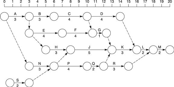
When preparing presentation or tender documents, or when the likelihood of the programme being changed is small, the main features of a network and bar chart can be combined in the form of a time scale network, or a linked bar chart. A time scale network has the length of the arrows drawn to a suitable scale in proportion to the duration of the activities. The whole network can, in fact, be drawn on a gridded background where each square of the grid represents a period of time such as a day, week, or month. Free float is easily ascertainable by inspection, but total float must be calculated in the conventional manner.
By drawing the activities to scale and starting each activity at the earliest date, a type of bar chart is produced that differs from the conventional bar chart in that some of the activity bars are on the same horizontal line. The disadvantage of such a presentation is that part of the network has to be redrawn ‘downstream’ from any activity that changes its duration. It can be seen that if one of the early activities changes in either duration or starting point, the whole network has to be modified.
However, a time scale network (especially if restricted to a few major activities) is a clear and concise communication document for reporting up. It loses its value in communicating down because changes increase with detail and constant revision would be too time consuming.
A further development of the Gantt chart, called a linked bar chart, is very similar to a normal bar chart, i.e., each activity is on a separate line and the activities are listed vertically at the edge of the paper. However, by drawing vertical lines connecting the end of one activity with the start of another, one can show the dependencies as a Gantt chart format. Unfortunately, these links, like the original bar charts, only show the implied relationship, as opposed to a critical path network, which shows the logically absolute relationship.
Chapter 24 describes the graphical analysis of networks, and it can be seen that if the ends of the activities were connected by the dummies a linked bar chart would result. This would, however, be based on the logic of the original AoA or AoN network.
Figure 19.39 shows a small time scale network and Figure 19.40 shows the same programme drawn as a linked bar chart.>

abcd