
Arithmetical Analysis and Floats
Abstract
Once a network has been drafted, it must be analyzed. Without a computer and in examinations, this must be done manually. This chapter discusses the common arithmetical methods for calculating the two main types of float (total and free) and the early and late starts and finishes and finding the critical path (or paths).The use of total and free float is fully described.
Keywords
Analysis; arithmetical analysis; total float; free float; critical path; early start and finish; late start and finish
Chapter Outline
Arithmetical Analysis
This method is the classical technique and can be performed in a number of ways. One of the easiest methods is to add up the various activity durations on the network itself, writing the sum of each stage in a square box at the end of that activity, i.e., next to the end event (Figure 21.1). It is essential that each route is examined separately and where the routes meet, the largest sum total must be inserted in the box. When the complete network has been summed in this way, the earliest starting will have been written against each event.
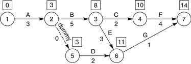
Now the reverse process must be carried out. The last event sum is now used as a base from which the activities leading into it are subtracted. The results of these subtractions are entered in triangular boxes against each event (Figure 21.2). As with the addition process for calculating the earliest starting times, a problem arises when a node is reached where two routes or activities meet. Since the latest starting times of an activity are required, the smallest result is written against the event.

The two diagrams are combined in Figure 21.3. The difference between the earliest and latest times gives the ‘float’, and if this difference is zero (i.e., if the numbers in the squares and triangles are the same) the event is on the critical path.

Figure 21.3
A table can now be prepared setting out the results in a concise manner (Table 21.1).
Table 21.1

Column a: activities by the activity titles. Column b: activities by the event numbers. Column c: activity durations, D. Column d: latest time of the activities’ end event, TLE. Column e: earliest time of the activities’ end event, TEE. Column f: earliest time of the activities’ beginning event, TEB. Column g: total float of the activity. Column h: free float of the activity.
Slack
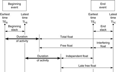
The difference between the latest and earliest times of any event is called ‘slack’. Since each activity has two events, a beginning event and an end event, it follows that there are two slacks for each activity. Thus the slack of the beginning event can be expressed as TLB – TEB and called beginning slack, and the slack of the end event, appropriately called end slack, is TLE – TEE. The concept of slack is useful when discussing the various types of float, since it simplifies the definitions.
Float
This is the name given to the spare time of an activity, and it is one of the more important by-products of network analysis. The four types of float possible will now be explained.
Total Float
It can be seen that activity 3–6 in Figure 21.3 must be completed after 13 time units, but can be started after 8 time units. Clearly, therefore, since the activity itself takes 3 time units, the activity could be completed in 8 + 3 = 11 time units. Therefore there is a leeway of 13–11 = 2 time units on the activity. This leeway is called total float and is defined as latest time of end event minus earliest time of beginning event minus duration, or TLE – TEB – D.
Figure 21.3 shows that total float is, in fact, the same as beginning slack. Also, free float is the same as total float minus end slack. The proof is given at the end of this chapter.
Total float has an important role to play in network analysis. By definition, it is the time between the anticipated start (or finish) of an activity and the latest permissible start (or finish).
The float can be either positive or negative. A positive float means that the operation or activity will be completed earlier than necessary, and a negative float indicates that the activity will be late. A prediction of the status of any particular activity is, therefore, a very useful and important piece of information for a manager. However, this information is of little use if not transmitted to management as soon as it becomes available, and every day of delay reduces the manager’s ability to rectify the slippage or replan the mode of operation.
The reason for calling this type of float ‘total float’ is because it is the total of all the ‘free floats’ in a string of activities when working back from where this string meets the critical path to the activity in question.
For example, in Figure 21.10, the activities in the lowest string J to P have the following free floats: J = 0, K = 10 – 9 = 1, L = 0, M = 15 – 14 = 1, N = 21 – 19 = 2, P = 0. Total float for K is therefore 2 + 1 + 1 + 1 = 4. This is the same as the 4 shown in the lower middle space of the node.
It is very easy to calculate the total floats and free floats in a precedence or Lester diagram. For any activity, the total float is the difference between the latest finish and earliest finish (or latest start and earliest start). The free float is the difference between the earliest finish of the activity in question and the earliest start of the following activity. Figure 21.15 makes this clear.
Calculation of Float
By far the quickest way to calculate the float of a particular activity is to do it manually. In practice, one does not need to know the float of all activities at the same time. A list of floats is, therefore, unnecessary. The important point is that the float of a particular activity that is of immediate interest is obtainable quickly and accurately.
Consider the string of activities in a simple construction process. This is shown in Figure 21.5 in activity on arrow (AoA) format and in Figure 21.6 in the simplified activity on node (AoN) format.
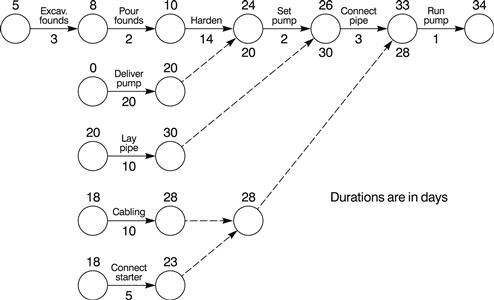
Figure 21.5

Figure 21.6
It can be seen that the total duration of the sequence is 34 days. By drafting the network in the method shown, and by using the day numbers at the end of each activity, including dummies, an accurate prediction is obtained immediately and the float of any particular activity can be seen almost by inspection. It will be noted that each activity has two dates or day numbers – one at the beginning and one at the end (Figure 21.7). Therefore, where two (or more) activities meet at a node, all the end day numbers are inserted (Figure 21.8). The highest number is now used to calculate the overall project duration, i.e., 30 + 3 = 33, and the difference between the highest and the other number immediately gives the float of the other activity and all the activities in that string up to the previous node at which more than one activity meet. In other words, ‘set pumps’ (Figure 21.5) has a float of 30 – 26 = 4 days, as have all the activities preceding it except ‘deliver pump’, which has an additional 24 – 20 = 4 days.
![]()
Figure 21.7
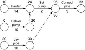
Figure 21.8
If, for example, the electrical engineer needs to know for how long he can delay the cabling because of an emergency situation on another part of the site, without delaying the project, he can find the answer right away. The float is 33 – 28 = 5 days. If the labour he needs for the emergency can be drawn from the gang erecting the starters, he can gain another 28 – 23 = 5 days. This gives him a total of 10 days’ grace to start the starter installation without affecting the total project time.
A few practice runs with small networks will soon emphasize the simplicity and speed of this method. We have in fact only dealt in this exposition with small – indeed, tiny – networks. How about large ones? It would appear that this is where the computer is essential, but, in fact, a well-drawn network can be analysed manually just as easily whether it is large or small. Provided the very simple base rules are adhered to, a very fast forward pass can be inserted. The float of any string can then be seen by inspection, i.e., by simply subtracting the lower node number from the higher node number, which forms the termination point of the string in question. This point can best be illustrated by the example given in Figure 21.9. For simplicity, the activities have been given letters instead of names, since the importance lies in understanding the principle, and the use of letters helps to identify the string of activities. In this example there are 50 activities. Normally, a practical network should have between 200 and 300 activities maximum (i.e., four to six times the number of activities shown), but this does not pose any greater problem. All the times (day numbers) were inserted, and the floats of activities in strings A, B, C, E, F, G, and H were calculated in 5 minutes. A 300-activity network would, therefore, take 30 minutes.

Figure 21.9
It can in fact be stated that any practical network can be ‘timed’, i.e., the forward pass can be inserted and the important float reported in 45 minutes. It is, furthermore, very easy to find the critical path. Clearly, it runs along the strings of activities with the highest node times. This is most easily calculated by working back from the end. Therefore the path runs through Aj, Ah, dummy, Dh, Dg, Df, De, Dd, Dc, Db, and Da.
An interesting little problem arises when calculating the float of activity Ce, since there are two strings emanating from the end node of that activity. By conventional backward pass methods – and indeed this is how a computer carries out the calculation – one would insert the backward pass in the nodes starting from the end (see Figure 21.10). When arriving at Ce, one finds that the latest possible time is 40 when calculating back along string Cg–Cf, while it is 38 when calculating back along string Ag–Af. Clearly, the actual float is the difference between the earliest date and the earliest of the two latest dates, i.e., day 38 instead of day 40. The float of Ce is therefore 38 – 21 = 17 days.

Figure 21.10
As described above, the calculation is tedious and time consuming. A far quicker method is available by using the technique shown in Figure 21.9, i.e., one simply inserts the various forward passes on each string and then looks at the end node of the activity in question – in our case, activity Ce. It can be seen that by following the two strings emanating from Ce that string Af–Ag joins Ah at day 36. String Cf–Cg, on the other hand, joins Ah at day 34. The float is, therefore, the smallest difference between the highest day number and one of the two day numbers just mentioned. Clearly, therefore, the float of activity Ce is 53 – 36 = 17 days. Cf and Cg, of course, have a float of 53 – 34 = 19 days.
The time to inspect and calculate the float by the second method is literally only a few minutes. All one has to do is to run through the paths emanating from the end node of the selected activity and note the highest day number where the strings meet the critical path. The difference between the day number of the critical string and the highest number on the tributary strings (emanating from the activity in question) is the float.
Supposing we now wish to find the float of activity Gb:
| String Gf–Gh meets Aj at day | 45. |
| String Ef–Eg meets Ah at day | 36. |
| Therefore the float is either | 56 – 45 = 11 |
| or | 53 – 36 = 17. |
Clearly, the correct float is 11 since it is the smaller of the two. The time taken to inspect and calculate the float was exactly 21 seconds!
All the floats calculated above have been total floats. Free float can only occur on activities entering a node when more than one enters that node. It can be calculated very easily by subtracting the total float of the incoming activity from the total float of the outgoing activity, as shown in Figure 21.11. It should be noted that one of the activities entering the node must have zero free float.

Figure 21.11
When more than one activity leaves a node, the value of the free float to be subtracted is the lowest of the outgoing activity floats, as shown in Figure 21.12.
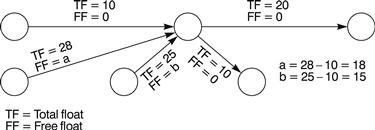
Figure 21.12
Free Float
Some activities, e.g., 5–6, as well as having total float have an additional leeway. It will be noted that activities 3–6 and 5–6 both affect activity 6–7. However, one of these two activities will delay 6–7 by the same time unit by which it itself may be delayed. The remaining activity, on the other hand, may be delayed for a period without affecting 6–7. This leeway is called free float, and can only occur in one or more activities where several meet at one event, i.e., if x activities meet at a node, it is possible that x – 1 of these have free float. This free float may be defined as earliest time of end event minus earliest time of beginning event minus duration, or TEE – TEB – D.
The Concept of Free Float
Students often find it difficult to understand the concept of free float. The mathematical definitions are unhelpful, and the graphical representation of Figure 21.4 can be confusing. The easiest way to understand the difference between total float and free float is to inspect the end node of the activity in question. As stated earlier, free float can only occur where two or more activities enter a node. If the earliest end times (i.e., the forward pass) for each individual activity are placed against the node, the free float is simply the difference between the highest number of the earliest time on the node and the number of the earliest time of the activity in question.
In the example given in Figure 21.13 the earliest times are placed in squares, so following the same convention it can be seen from the figure (which is a redrawing of Figure 21.1 with all the earliest and latest node times added) that:
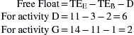
Figure 21.14 shows the equivalent precedence (AoN) diagram from which the free float can be easily calculated by subtracting the early finish time of the preceding node from the early start time of the succeeding node.
![]()
![]()

Figure 21.13
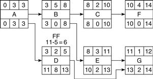
Figure 21.14
Activity E, because it is not on the critical path, has total float of 13 – 11 = 2 but has no free float.
The check of the free float by the formal definition is as follows:
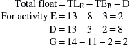
The check of the total float by the formal definitions is as follows:
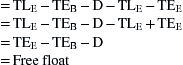
It was stated earlier that total float is the same as beginning slack. This can be shown by rewriting the definition of total float = TLE – TEB – D as total float = TLE – D – TEB but TLE – D = TLB. Therefore:
![]()
To show that free float = total float – end slack, consider the following definitions:
![]() (21.A)
(21.A)
![]() (21.B)
(21.B)
![]() (21.C)
(21.C)
Subtracting equation (21.C) from equation (21.B):
 (21.A)
Therefore:
![]()
If a computer is not available, free float on an arrow diagram can be ascertained by inspection, since it can only occur where more than one activity meets a node. This was described in detail earlier with Figures 21.5 and 21.6. If the network is in the precedence format, the calculation of free float is even easier. All one has to do is to subtract the early finish time in the preceding node from the early start time of the succeeding node. This is clearly shown in Figure 21.15, which is the precedence equivalent to Figure 21.5.

One of the phenomena of a computer printout is the comparatively large number of activities with free float. Closer examination shows that the majority of these are in fact dummy activities. The reason for this is, of course, obvious, since, by definition, free float can only exist when more than one activity enters a node. As dummies nearly always enter a node with another (real) activity, they all tend to have free float. Unfortunately, no computer program exists that automatically transfers this free float to the preceding real activity, so the benefit of the free float is not immediately apparent and is consequently not taken advantage of.
Interfering Float
The difference between the total float and the free float is known as interfering float. Using the previous notation, this can be expressed as
![]()
i.e., as the latest time of the end event minus the earliest time of the end event. It is, therefore, the same as the end slack.
Independent Float
The difference between the free float and the beginning slack is known as independent float:

This problem does not exist with precedence diagrams as there are no dummy activities in this network format.
Thus independent float is given by the earliest time of the end event minus the latest time of the beginning event minus the duration.
In practice neither the interfering float nor the independent float find much application, and for this reason they will not be referred to in later chapters. The use of computers for network analysis enables these values to be produced without difficulty or extra cost, but they only tend to confuse the user and are therefore best ignored.
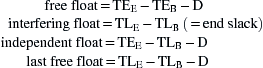
Summarizing all the above definitions, Figure 21.4 and the following expressions may be of assistance.
Definitions
![]()
Because float is such an important part of network analysis and because it is frequently quoted – or misquoted – by computer protagonists as another reason why computers must be used, a special discussion of the subject may be helpful to those readers not too familiar with its use in practice.
Of the three types of float shown on a printout, i.e., the total float, free float, and independent float, only the first – the total float – is in general use. Where resource smoothing is required, a knowledge of free float can be useful, since the activities with free float can be moved backwards or forwards in time without affecting any other activities. Independent float, on the other hand, is really quite a useless piece of information and should be suppressed (when possible) from any computer printout. Of the many managers, site engineers, and planners interviewed, none has been able to find a practical application of independent float.
Critical Path
Some activities have zero total float, i.e., no leeway is permissible for their execution, hence any delays incurred on the activities will be reflected in the overall project duration. These activities are therefore called critical activities, and every network has a chain of such critical activities running from the beginning event of the first activity to the end event of the last activity, without a break. This chain is called the critical path.
Frequently a project network has more than one critical path, i.e., two or more chains of activities all have to be carried out within the stipulated duration to avoid a delay to the completion date. In addition, a number of activity chains may have only one or two units of float, so that, for all intents and purposes, they are also critical. It can be seen, therefore, that it is important to keep an eye on all activity chains that are either critical or near-critical, since a small change in duration of one chain could quickly alter the priorities of another.
One disadvantage of the arithmetical method of analysis using the table or matrix shown in Table 21.1 is that all the floats must be calculated before the critical path can be ascertained. This method (which has only been included for historical interest) is very laborious and is therefore not recommended.
In any case, this drawback is eliminated when the method of analysis shown in Figure 21.9 is employed.
Critical Chain Project Management (CCPM)
This planning technique differs from conventional CPA in that resource restraints and dependencies are considered as well as operation logic. This requires buffers to be introduced to allow for possible resource issues. Progress monitoring can then carried out by measuring the rate at which the buffers are used up instead of just recording the individual task performance.
In practice this method is probably most appropriate where resources are not easily assessable at the planning stage. Contingencies in the form of buffers must therefore be incorporated, with the result that the overall duration will probably be longer, and as a consequence the planned completion date will more likely be met.
In the construction industry, where the program completion date is often set by the client, i.e., the opening of a venue or start of production, the project program will be based on the construction logic of the operational activities, which must then be provided with the necessary resources (plant, material, and labour) to carry out the work. It is inconceivable that at the start of a project a contractor in the construction industry would tell his or her client that the project cannot be completed by the specified date because the necessary resources cannot be obtained.