
Control Graphs and Reports
Abstract
Here the relationship between networks and EVA is demonstrated by an example of a boiler construction project. The network, which is shown in AoA and AoN format, has been converted into a bar chart with the manhours added. These hours were then transferred to an earned value analysis sheet, from which curves were generated showing the movement and trends of the actual hours, value hours (earned value), estimated final hours, % complete and % efficiency. The jargon terms BCWP, BCWS, ACWP, CPI, SPI, ATE, and BAC have been explained and compared with the equivalent non-jargon terms and calculations have been provided to show how to obtain these. A sample time sheet for feedback of EVA data has been included
Keywords
EVA; BCWP; BCWS; ACWP; CPI; SPI; control graphs. % complete. % efficiency; Time sheets
Chapter Outline
Apart from the numerical report shown in Figure 33.5, two very useful management control graphs can then be produced:
1. Showing budget hours, actual hours, value hours, and predicted final hours, all against a common time base;
2. Showing percentage planned, percentage complete, and efficiency, against a similar time base.
The actual shape of the curves on these graphs give the project manager an insight into the running of the job, enabling appropriate action to be taken.
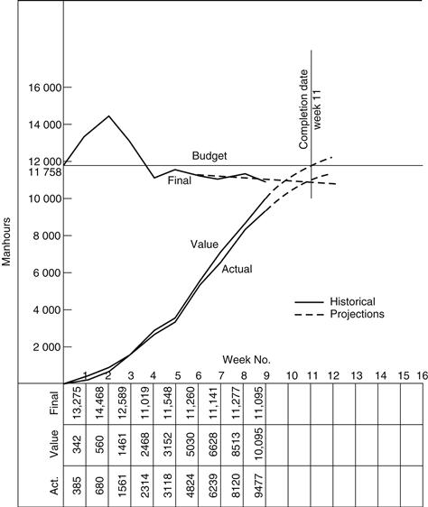
Figure 33.1 shows the site returns of manhours of a small project over a nine-month period, and, for convenience, the table of percentage complete and actual and value hours has been drawn on the same page as the resulting curves. In practice, the greater number of activities would not make such a compressed presentation possible.

A number of interesting points are ascertainable from the curves:
1. There was obviously a large increase in site labour between the fifth and sixth months, as is shown by the steep rise of the actual hours curve.
2. This has resulted in increased efficiency.
3. The learning curve given by the estimated final hours has flattened in month 6 making the prediction both consistent and realistic.
4. Month 7 showed a divergence of actual and value hours (indicated also by a loss of efficiency), which was corrected (probably by management action) by month 8.
5. It is possible to predict the month of actual completion by projecting all the curves forward. The month of completion is then given:
(a) When the value hours curve intersects the budget line; and
(b) When the actual hours curve intersects the estimated final hours curve.
In this example, one could safely predict completion of the project in month 10.
It will be appreciated that this system lends itself ideally to computerization, giving the project manager the maximum information with the very minimum of site input. The sensitivity of the system is shown by the immediate change in efficiency when the value hours diverged from the actual hours in month 7. This alerts management to investigate and apply corrections.
For maximum benefit the returns and calculations should be carried out weekly. By using the normal weekly time cards very little additional site effort is required to complete the returns, and with the aid of a good computer program the results should be available 24 hours after the returns are received.
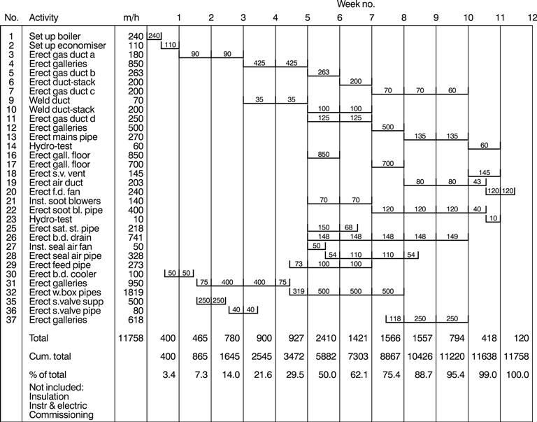
An example of the application of a manual EVA analysis is shown in Figures 33.2 to 33.9. The site construction network of a package boiler installation is given in Figure 33.2. Although the project consisted of three boilers, only one network, that of Boiler No. 1 is shown. In this way it was possible to control each boiler construction separately and compare performances. The numbers above the activity description are the activity numbers, while those below are the durations. The reason for using activity numbers for identifying each activity, instead of the more conventional beginning and end event numbers, is that the identifier must always be uniquely associated with the activity description.

If the event numbers (in this case the coordinates of the grid) were used, the identifier could change if the logic were amended or other activities were inserted. In a sense, the activity number is akin to the node number of a precedence diagram, which is always associated with its activity. The use of precedence diagrams and computerized EVA is therefore a natural marriage, and to illustrate this point, a precedence diagram is shown in Figure 33.3.

Once the network has been drawn, the manhours allocated to each activity can be represented graphically on a bar chart. This is shown in Figure 33.4. By adding up the manhours for each week, the totals, cumulative totals, and each week’s percentage of the total manhours can be calculated. If these percentages are then plotted as a graph the planned percentage complete curve can be drawn. This is shown in Figure 33.7.
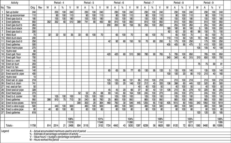

All the work described up to this stage can be carried out before work starts on-site. The only other operation necessary before the construction stage is to complete the left-hand side of the site returns analysis sheet. This is shown in Figure 33.5, which covers only periods 4 to 9 of the project. The columns to be completed at this stage are:
Once work has started on-site, the construction manager reports weekly on the progress of each activity worked on during that week. All he has to state is:
If the computation is carried out manually, the figures are entered on the sheet (Figure 33.5) and the following values calculated weekly:
1. Total manhours expended this week (W column)
2. Total manhours to date (A column)
3. Percentage complete of project (% column)
Alternatively, the site returns can be processed by computer and the resulting printout of part of a project is shown in Figure 33.8. Whether the information is collected manually or electronically, the return can be made on a standard timesheet with the only addition being a % complete column. In other words, no additional forms are required to collect information for EVA. There are in fact only three items of data to be returned to give sufficient information:
1. The activity number of the activity actually being worked on in that time period
2. The actual hours being expended on each activity worked on in that time period

All the other information required for computation and reporting (such as activity titles and activity manhour budgets) will already have been inputted and is stored in the computer. A typical modified timesheet is shown in Figure 33.9.

A complete set of printouts produced by a modern project management system are shown in Figures 33.10 to 33.14. It will be noted that the network in precedence format has been produced by the computer, as have the bar chart and curves. In this program the numerical EVA analysis has been combined with the normal critical path analysis from one database, so that both outputs can be printed and updated at the same time on one sheet of paper. The reason the totals of the forecast hours are different from the manual analysis is that the computer calculates the forecast hours for each activity and then adds them up, while in the manual system the total forecast hours are obtained by simply dividing the actual hours by the percentage complete rounded off to the nearest 1%.


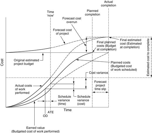
Figure 33.15 Earned Value Chart reproduced from BS 6079 ‘Guide to Project Management’ by permission of British Standards Institution.
As mentioned earlier, if the budget hours, actual hours, value hours, and estimated final hours are plotted as curves on the same graph, their shape and relative positions can be extremely revealing in terms of profitability and progress. For example, it can be seen from Figure 33.6 that the contract was potentially running at a loss during the first three weeks, since the value hours were less than the actual hours. Once the two curves crossed, profitability returned and in fact increased, as indicated by the diverging nature of the value and actual hour curves. This trend is also reflected by the final hours curve dipping below the budget hour line.
The percentage-time curves in Figure 33.7 enable the project manager to compare actual percentage complete with planned percentage complete. This is a better measure of performance than comparing actual hours expended with planned hours expended. There is no virtue in spending the manhours in accordance with a planned rate. What is important is the percentage complete in relation to the plan and whether the hours spent were useful hours. Indeed, there should be every incentive to spend less hours than planned, provided that the value hours are equal or greater than the actual, and the percentage complete is equal or greater than the planned.
The efficiency curve in Figure 33.7 is useful, since any drop is a signal for management action. Curve ‘A’ is based on the efficiency calculated by dividing the cumulative value hours by the cumulative actual hours for every week. Curve ‘W’ is the efficiency by dividing the value hours generated in a particular week by the actual hours expended in that week. It can be seen that Curve ‘W’ (shown only for the periods 5 to 9) is more sensitive to change and is therefore a more dramatic warning device to management.
Finally, by comparing the curves in Figures 33.6 and 33.7 the following conclusions can be drawn:
1. Value hours exceed actual hours (Figure 33.6). This indicates that the site is efficiently run.
2. Final hours are less than budget hours (Figure 33.6). This implies that the contract will make a profit.
3. The efficiency is over 100% and rising (Figure 33.7). This bears out conclusion 1.
4. The actual percentage complete curve (Figure 33.7), although less than the planned, has for the last four periods been increasing at a greater rate than the planned (i.e., the line is at a steeper angle). Hence the job may well finish earlier than planned (probably in Week 11).
5. By projecting the value hour curve forward to meet the budget hour line, it crosses in Week 11 (Figure 33.6).
6. By projecting the actual hour curve to meet the projection of the final hour curve, it intersects in Week 11 (Figure 33.6). Hence Week 11 is the probable completion date.
The computer printout shown in Figure 33.8 is updated weekly by adding the manhours logged against individual activities. However, it is possible to show on the same report the cost of both the historical and current manhours. This is achieved by feeding the average manhour rate for the contract into the machine at the beginning of the job and updating it when the rate changes. Hence the new hours will be multiplied by the current rates. A separate report can also be issued to cover the indirect hours such as supervision, inspection, inclement weather, general services, etc.
Since the value hour concept is so important in assessing the labour content of a site or works operation, the following summary showing the computation in non-numerical terms may be of help:
If
| B | = Budget hours (total) |
| C | = Actual hours (total) |
| D | = % complete |
| E | = Value hours (earned value) (total) |
| F | = Forecast final hours |
| G | = Efficiency % (CPI) |
Then:
![]()
Overall Project Completion
Once the manhours have been ‘costed’ they can be added to other cost reports of plant, equipment, materials, subcontracts, etc., so that an overall percentage completion of a project can be calculated for valuation purposes on the only true common denominator of a project – money.
The total value to date divided by the revised budget × 100 is the percentage complete of a job. The value hour concept is entirely compatible with the conventional valuation of costing such as value of concrete poured, value of goods installed, cost of plant utilized – activities, which can, by themselves, be represented on networks at the planning stage.
Table 33.1 shows how the two main streams of operations, i.e., those categories measured by cost and those measured by manhours can be combined to give an overall picture of the percentage completion in terms of cost and overall cost of a project. While the operations shown relate to a construction project, a similar table can be drawn for a manufacturing process, covering such operations as design, tooling, raw material purchase, machinery, assembly, testing, packing, etc.
Table 33.1

Cost of overheads, plant amortization, licences, etc., can, of course, be added like any other commodity. An example giving quantities and cost values of a small job involving all the categories shown in Table 33.1 is presented in Tables 33.2 to 33.4. It can be seen that in order to enable an overall percentage complete to be calculated, all the quantities of the estimate (Table 33.2) have been multiplied by their respective rates – as in fact would be done as part of any budget – to give the estimated costs.

Table 33.3 shows the progress after a 16-week period, but in order to obtain the value hours (and hence the cost value) of Category D it was necessary to break down the manhours into work packages that could be assessed for percentage completion. Thus, in Table 33.4, the pipelines A and B were assessed as 35% and 45% complete, respectively, and the pump and tank connections were found to be 15% and 20% complete, respectively. Once the value hours (3180) were found, they could be multiplied by the average cost per manhour to give a cost value of $14628.

Table 33.4
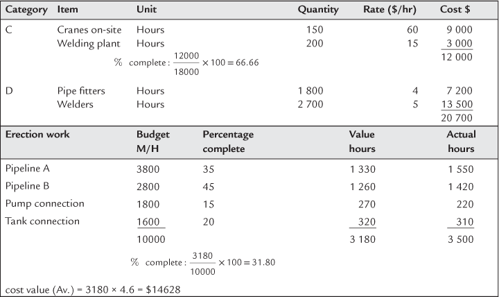
Table 33.5 shows the summary of the four categories. An adjustment should therefore also be made to the value of plant utilization Category C since the two are closely related. The adjusted value total would therefore be as shown in Column V.

With a true value of expenditure to date of $104,048, the percentage completion in terms of cost of the whole site is therefore:
![]()
It must be stressed that the of cost completed is not the same as the completion of construction work. It is only a valuation method when the material and equipment are valued (and paid for) in their month of arrival or installation.
When the materials or equipment are paid for as they arrive on site (possibly a month before they are actually erected), or when they are supplied ‘free issue’ by the employer, they must not be part of the value or complete calculation.
It is clearly unrealistic to include materials and equipment in the complete and efficiency calculation as the cost of equipment is not proportional to the cost of installation. For example, a carbon steel tank takes the same time to lift onto its foundations as a stainless steel tank, yet the cost is very different! Indeed, in some instances, an expensive item of equipment may be quicker and cheaper to install than an equivalent cheaper item, simply because the expensive item may be more ‘complete’ when it arrives on site.
All the items in the calculations can be stored, updated, and processed by computer, so there is no reason why an accurate, up-to-date, and regular progress report cannot be produced on a weekly basis, where the action takes place – on the site or in the workshop.
Clearly, with such information at one’s fingertips, costs can truly be controlled – not merely reported!
It can be seen that the value hours for erection work are only 3180 against an actual manhours usage of 3500. This represents an efficiency of only
![]()
An adjustment should therefore also be made to the value of plant utilization, i.e., 12000 × 91% = 10,920. The adjusted value total would therefore be as shown in column V.
The SMAC system described on the previous pages was developed in 1978 by Foster Wheeler Power Products, primarily to find a quicker and more accurate method for assessing the % complete of multi-discipline, multi-contractor construction projects.
However, about 10 years earlier the Department of Defense in the USA developed an almost identical system called Cost, Schedule, Control System (CSCS), which was generally referred to as Earned Value Analysis (EVA). This was mainly geared to the cost control of defence projects within the USA, and apart from UK subcontractors to the American defence contractors, was not disseminated widely in the UK.
While the principles of SMAC and EVA are identical, there developed inevitably a difference in terminology, which has caused considerable confusion to students and practitioners. Figure 33.16 lists these abbreviations and their meaning, and Figure 33.17 shows the comparison between the now accepted EVA ‘English’ terms (shown in bold) and the CSCS jargon (shown in italics).

Figure 33.16

The CSCS also introduced four new parameters for cost efficiency and, for want of a better word, time efficiency:
1. The cost variance: this is the arithmetical difference at any point between the earned value and the actual cost.
2. The schedule variance: this is the arithmetical difference between the earned value and the scheduled (or planned) cost. However, comparing progress in time by subtracting the planned cost from the earned value is somewhat illogical as both are measured in monetary terms. It would make more sense to use parameters measured in time to calculate the time variance. This can be achieved by subtracting the actual duration (ATE) for a particular earned value from the originally planned duration (OD) for that earned value. This is shown clearly in Figure 33.15. It can be seen that if the project is late, the result will be negative. There are therefore two schedule variances (SV):
(a) SV (cost), which is measured on the cost scale of the graph;
(b) SV (time), which is measured on the time scale.
3. The cost efficiency is called the cost performance index (CPI) and is
4. The ‘time efficiency’ is called the schedule performance index (SPI) and is
earned value/scheduled (or planned) cost.
Again, as with the schedule variance, measuring efficiency in time by dividing the earned value by the planned cost, which are both measured in monetary terms or manhours, is equally illogical and again it would be more sensible to use parameters measured in time. Therefore by dividing the planned duration for a particular earned value by the actual duration for that earned value a more realistic index can be calculated. All time measurements must be in terms of hours, day numbers, week numbers, etc. – not calendar dates!
There are therefore now two SPIs:
(a) SPI (cost) measured on the cost scale, i.e., earned value/scheduled cost;
(b) SPI (time) measured on the time scale, i.e., planned duration/actual duration.
In practice, the numerical difference between these two quotients is small, so that SPI (cost), which is easier to calculate, is sufficient for most purposes, bearing in mind that the result is still only a prediction based on historical data.
In 1996 the National Security Industrial Association (NISA) of America published their own Earned Value Management System (EVMS), which dropped the terms such as ACWP, BCWP, and BCWS used in CSCS and adopted the simpler terms of Earned Value, Actual, and Schedule instead.
Since then the American Project Management Institute (PMI), the British Association for Project Management (APM), and the British Standards Institution (BSI) have all discarded the CSCS abbreviations and have also adopted the full English terms. In all probability this will be the future universal terminology.
Figure 33.17 clearly shows the earned value terms in both English (in bold) and EV jargon (in italics).
Earned Schedule
It has long been appreciated that Schedule Performance Index (cost) (SPI cost) based on the cost differences of the earned value and planned curves is somewhat illogical. An index reflecting schedule changes should be based on the time differences of a project. For this reason Schedule Performance Index (time) (SPI time) is a more realistic approach and gives more accurate results, although in practice the numerical differences between SPI cost and SPI time are not very great. SPI time for any point in time or ‘time now’ can be obtained graphically by dropping a vertical line from the planned curve to the time base line, from the point of the curve where the planned value is equal to the earned value for the selected ‘time now’. This SPI time is in effect the time efficiency of the project and has therefore been sometimes referred to ‘earned schedule’.
In the same way that Budget Cost / CPI = the final predicted cost,
![]()
It goes without saying that all units on the time scale must be in day, week, or month numbers, not in calendar dates!
Integrated Computer Systems
Until 1992, the EVA system was run as a separate computer program in parallel with a conventional CPM system. Now, however, a number of software companies have produced project management programs that fully integrate critical path analysis with earned value analysis. One of the best programs of this type, Primavera P6, is fully described in Chapter 51.
The system can, of course, be used for controlling individual work packages, whether carried out by direct labour or by subcontractors, and by multiplying the total actual manhours by the average labour rate, the cost to date is immediately available. The final results should be carefully analysed and can form an excellent base for future estimates.
As previously stated, apart from printing the EVA information and the conventional CPM data, the program also produces a computer drawn network. This is drawn in precedence format.
The information shown on the various reports include:
1. The manhours spent on any activity or group of activities
2. The % complete of any activity
3. The overall % complete of the total project
4. The overall manhours expended
5. The value (useful) hours expended
6. The efficiency of each activity
8. The estimated final hours for completion
9. The approximate completion date
10. The manhours spent on extra work
11. The relationship between programme and progress
12. The relative performance of subcontractors or internal subareas of work