11. Enhancing Pivot Table Reports with Macros
Why Use Macros with Your Pivot Table Reports?
Imagine that you could be in multiple locations at one time, with multiple clients at one time, helping them with their pivot table reports. Suppose you could help multiple clients refresh their data, extract top 20 records, group by months, or sort by revenue The fact is you can do just that by using Excel macros.
A macro is a series of keystrokes that have been recorded and saved. After saved, the macro can be played back on command. In other words, you can record your actions in a macro, save the macro, and then allow your clients to play back your actions with the touch of a button. It would be as though you were there with them! This functionality is exceptionally useful when you’re distributing pivot table reports.
For example, suppose you want to give your clients the option of grouping their pivot table report by month, quarter, or year. Although the process of grouping can be technically performed by anyone, some of your clients might not have a clue how to do it. In this case, you could record a macro to group by month, a macro to group by quarter, and a macro to group by year. Then, you could create three buttons, one for each macro. In the end, your clients, having little experience with pivot tables, need only to click a button to group their pivot table report.
A major benefit of using macros with your pivot table reports is the power you can give your clients to easily perform pivot table actions that they would not normally be able to perform on their own, empowering them to more effectively analyze the data you provide.
Recording Your First Macro
Look at the pivot table in Figure 11.1. You know that you can refresh this pivot table by right-clicking inside the pivot table and selecting Refresh Data. Now, if you were to record your actions with a macro while you refreshed your pivot table, you, or anyone else, could replicate your actions and refresh this pivot table by running the macro.
Figure 11.1 This basic pivot table can easily be refreshed by right-clicking and selecting Refresh Data, but if you recorded your actions with a macro, you could also refresh this pivot table simply by running the macro.

The first step in recording a macro is to initiate the Record Macro dialog box. Select the Developer tab on the Ribbon, and then select Record Macro.
Tip
Can’t find the Developer tab on the Ribbon? Click the File tab on the Ribbon, and then select the Options selection. This opens the Excel Options dialog box, where you click Customize Ribbon. In the ListBox to the far right, you select the Developer check box. Selecting this option enables the Developer tab.
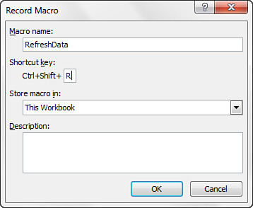
When the Record Macro dialog box activates, you can fill in a few key pieces of information about the macro:
• Macro Name—Enter a name for your macro. You should generally enter a name that describes the action being performed.
• Shortcut Key—You can enter any letter into this input box. That letter becomes part of a set of keys on your keyboard that can be pressed (in conjunction with the Ctrl key) to play back the macro. This is optional.
• Store Macro In—Specify where you want the macro to be stored. If you are distributing your pivot table report, you should select This Workbook so that the macro is available to your clients.
• Description—In this input box, you can enter a few words that give more detail about the macro.
Because this macro refreshes your pivot table when it is played, name your macro RefreshData. Also assign a shortcut key of R. Notice that the dialog box gives you a full key of Ctrl+Shift+R. Keep in mind that you use the full key to play your macro after it is created. Be sure to store the macro in This Workbook. Click OK to continue. When this is done, your dialog box should look like the one shown in Figure 11.2.
Figure 11.2 Fill in the Record Macro dialog box as shown here, and then click OK to continue.
When you click OK in the Record Macro dialog box, you initiate the recording process. At this point, any action you perform is being recorded by Excel. In that case, you want to record the process of refreshing your pivot table.
Right-click anywhere inside the pivot table, and then select Refresh Data. After you have refreshed your pivot table, you can stop the recording process by going up to the Developer tab and selecting the Stop Recording button.
Congratulations! You have just recorded your first macro. You can now play your macro by pressing Ctrl+Shift+R.
Note
In Excel 2010, Microsoft has enhanced the security model to remember files that you’ve deemed trustworthy. That is, when you open an Excel workbook and click the Enable button, Excel remembers that you trusted that file. Each time you open the workbook after that, Excel automatically trusts it.
For information on macro security in Excel 2010, pick up Que Publishing’s Microsoft Excel 2010 In Depth by Bill Jelen (ISBN 0789743086).
Creating a User Interface with Form Controls
Allowing your clients to run your macro with shortcut keys like Ctrl+Shift+R can be a satisfactory solution if you have only one macro in your pivot table report. However, suppose you want to allow your clients to perform several macro actions. In this case, you should give your clients a clear and easy way to run each macro without having to remember a gaggle of shortcut keys. A basic user interface provides the perfect solution. You can think of a user interface as a set of controls such as buttons, scrollbars, and other devices that enable users to run macros with a simple click of the mouse.
In fact, Excel offers a set of controls designed specifically for creating user interfaces directly on a spreadsheet. These controls are called form controls. The general idea behind form controls is that you can place one on a spreadsheet and then assign a previously recorded macro to it. After a macro is assigned to the control, that macro is executed, or played, when the control is clicked.
Form controls can be found in the Controls group on the Developer tab. To get to the form controls, simply select the Insert icon in the Controls group, as demonstrated in Figure 11.3.
Figure 11.3 To see the available form controls, click Insert in the Controls group on the Developer tab.
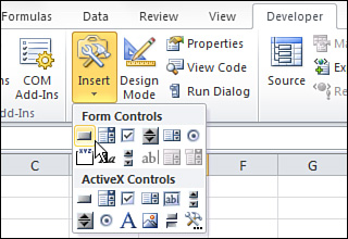
Here, you can select the control that best suits your needs. In this example, you want your clients to be able to refresh their pivot table with the click of a button. Click the Button control, and then drop the control onto your spreadsheet by clicking the location you would like to place the button.
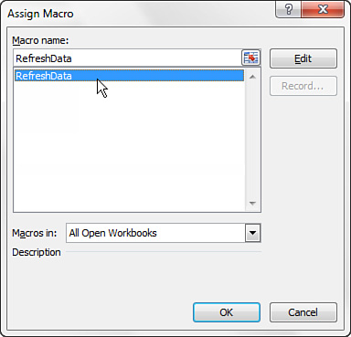
After you drop the button control onto your spreadsheet, the Assign Macro dialog box, as shown in Figure 11.4, opens and asks you to assign a macro to this button. Select the macro you want to assign to the button, in this case RefreshData, and then click OK.
Figure 11.4 Select the macro you want to assign to the button, and then click OK. In this case, you want to select RefreshData.
Note
Notice that there are form controls and ActiveX controls. Although they look similar, they are quite different. Form controls, with their limited overhead and easy configuration settings, are designed specifically for use on a spreadsheet. Meanwhile, ActiveX controls are typically used on Excel userforms. As a general rule, you always want to use form controls when working on a spreadsheet.
Note
Keep in mind that all the controls in the Forms toolbar work in the same way as the command button; in that, you assign a macro to run when the control is selected.
As you can see in Figure 11.5, you can assign each macro in your workbook to a different form control, and then name the controls to distinguish between them.
Figure 11.5 You can create a different button for each one of your macros.
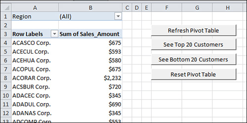
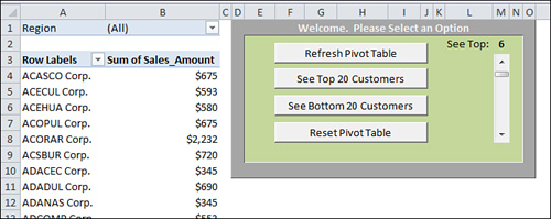
Figure 11.6 demonstrates that after you have all the controls you need for your pivot table report, you can format the controls and surrounding spreadsheet to create a basic interface.
Figure 11.6 You can easily create the feeling of an interface with a handful of macros, a few form controls, and a little formatting.
Altering a Recorded Macro to Add Functionality
When you record a macro, Excel creates a module that stores the recorded steps of your actions. These recorded steps are actually lines of Visual Basic for Applications (VBA) code that make up your macro. You can add some interesting functionality to your pivot table reports by tweaking your macro’s VBA code to achieve various effects.
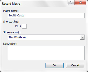
To get a better understanding of how this process works, start by creating a new macro that extracts the top five records by customer. Go to the Developer tab, and select Record Macro. Set up the Record Macro dialog box, as shown in Figure 11.7. Name your new macro TopNthCusts, and specify that you want to store the macro in This Workbook. Click OK to start recording.
Figure 11.7 Name your new macro, and then specify where you want to store it.
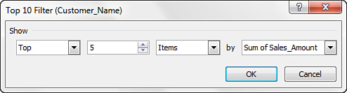
After you have started recording, right-click the Customer field and select Filter. Then, select Top 10. Selecting this option opens the Filter dialog box, where you specify that you want to see the top five customers by sales amount. Enter the settings shown in Figure 11.8, and then click OK.
Figure 11.8 Enter the settings you see here to get the top five customers by revenue.
After successfully recording the steps to extract the top five customers by revenue, select Stop Recording from the Developer tab.
You now have a macro that, when played, filters your pivot table to the top five customers by revenue. The plan is to tweak this macro to respond to a scrollbar. That is, you force the macro to base the number used to filter the pivot table on the number represented by a scrollbar in your user interface. In other words, a user can get the top 5, top 8, or top 32 simply by moving a scrollbar up or down.
To get a scrollbar onto your spreadsheet, select the Insert icon on Developer tab, and then select the scrollbar control from the form controls. Place the scrollbar control onto your spreadsheet by clicking the location you would like to see it.
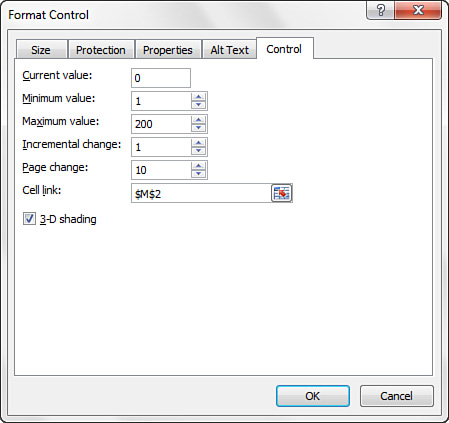
Right-click the scrollbar, and then select Format Control. This activates the Format Control dialog box. Here, you make the following setting changes: Set Minimum Level to 1 so the scrollbar cannot go below 1; set Maximum Level to 200 so the scrollbar cannot go above 200; and set Cell Link to $M$2 so that the number represented by the scrollbar outputs to cell M2. After you have completed these steps, your dialog box should look like the one shown in Figure 11.9.
Figure 11.9 After you have placed a scrollbar on your spreadsheet, configure the scrollbar as shown here.
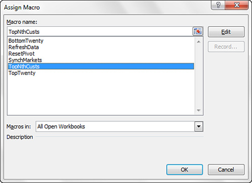
Next, assign the TopNthCusts macro you just recorded to your scrollbar, as demonstrated in Figure 11.10. Right-click the scrollbar, and then select Assign Macro. Select the TopNthCusts macro from the list, and then click OK. Assigning this macro ensures that it plays each time the scrollbar is clicked.
Figure 11.10 Select the macro from the list.
At this point, test your scrollbar by clicking on it. When you click your scrollbar, two things should happen: The TopNthCusts macro should play, and the number in cell M2 should change to reflect your scrollbar’s position. The number in cell M2 is important because that is the number you are going to reference in your TopNthCusts macro.
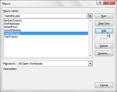
The only thing left to do is to tweak your macro to respond to the number in cell M2, effectively tying it to your scrollbar. To do this, you have to get to the VBA code that makes up the macro. There are several ways to get there, but for the purposes of this example, go to the Developer tab and select Macros. Selecting this option opens the Macro dialog box, exposing several options. From here, you can run, delete, step into, or edit a selected macro. To get to the VBA code that makes up your macro, select the macro, and then select Edit, as demonstrated in Figure 11.11.
Figure 11.11 To get to the VBA code that makes up the TopNthCusts macro, select the macro, and then select Edit.
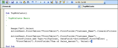
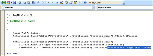
The Visual Basic Editor opens with a detailed view of all the VBA code that makes up this macro (see Figure 11.12). Notice that the number 5 is hard-coded as part of your macro. The reason is that you originally recorded your macro to filter the top five customers by revenue. Your goal here is to replace the hard-coded number 5 with the value in cell M2, which is tied to your scrollbar.
Figure 11.12 Your goal is to replace the hard-coded number 5, as specified when you originally recorded your macro, with the value in cell M2.
You delete the number 5 and replace it with the following:
ActiveSheet.Range("M2").Value
Your macro’s code should now look similar to the code shown in Figure 11.13.
Figure 11.13 Simply delete the hard-coded number 5 and replace it with a reference to cell M2.
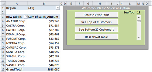
Close the Visual Basic Editor to get back to your pivot table report. Test your scrollbar by setting the scrollbar to 11. Your macro should play and filter out the Top 11 customers by revenue, as shown in Figure 11.14.
Figure 11.14 After a little formatting, you have a clear and easy way for your clients to get the top customers by revenue.
Case Study: Synchronizing Two Pivot Tables with One Combo Box
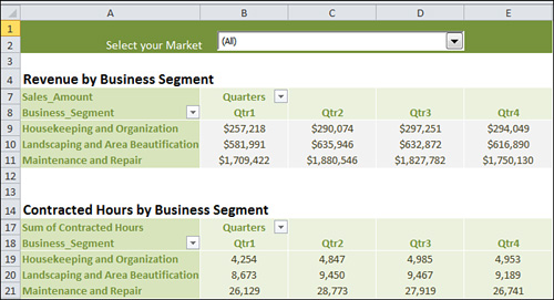
The report in Figure 11.15 contains two pivot tables. Each pivot table has a filter field to enable you to select a market. The problem is that every time you select a market from the filter field in one pivot table, you have to select the same market from the filter field in the other pivot table to ensure you are analyzing the correct Units Sold versus Revenue.
Figure 11.15 This pivot table report contains two pivot tables with filter fields that filter out a market. The issue is that you have to synchronize the two pivot tables when analyzing data for a particular market.
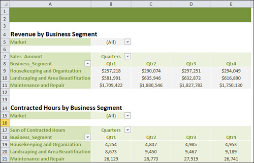
Not only is it a bit of a hassle to have to synchronize both pivot tables every time you want to analyze a new market’s data, but there is a chance you, or your clients, might forget to do so.
One way to synchronize these pivot tables is to use a combo box. The idea is to record a macro that selects a market from the Market field of both tables. Then you can create a combo box and fill it with the market names that exist in your two pivot tables. Finally, you can alter your macro to filter both pivot tables, using the value from your combo box. To do so, follow these steps:
1. Create a new macro and call it SynchMarkets. When recording starts, select the California market from the Market field in both pivot tables, and then stop recording.
2. Activate the Forms toolbar and place a combo box onto your spreadsheet.
3. Create a hard-coded list of all the markets that exist in your pivot table. Note that the first entry in your list is (All). You must include this entry if you want to select all markets with your combo box.
As you can see in Figure 11.16, you place the combo box and your list of markets directly in your spreadsheet.
Figure 11.16 At this point, you should have all the tools you need: a macro that changes the Market field of both pivot tables, a combo box on your spreadsheet, and a list of all the markets that exist in your pivot table.

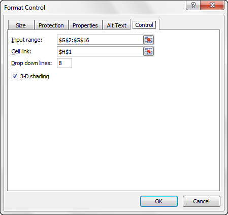
4. Right-click your combo box and select Format Control to perform the initial setup. First, specify an input range for the list you are using to fill your combo box. In this case, this means the market list you created in step 3. Next, specify a cell link—that is, the cell that shows the index number of the item you select. (Cell H1 is the cell link in this example.) After you have configured your combo box, your dialog box should look similar to the one shown in Figure 11.17.
Figure 11.17 The settings for your combo box should reference your market list as the input range and specify a cell link close to your market list. In this case, the cell link is cell H1.
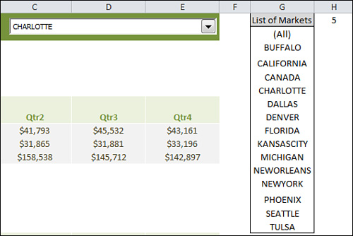
At this point, you should now be able to select a market from your combo box and see the associated index number in cell H1. Why an index number instead of the name of the selected market? Well, the only output of a combo box form control is an index number. This is the position number of the selected item. For instance, in Figure 11.18, the selection of Charlotte from the combo box results in the number 5 in cell H1. This means that Charlotte was the fifth item in the combo box.
Figure 11.18 Your combo box, now filled with market names, outputs an index number in cell H1 when a market is selected.
To make use of this index number, you have to pass it through the INDEX function. The INDEX function converts an index number to a value that can be recognized.
5. Enter an INDEX function that converts the index number in cell H1 to a value (See Figure 11.19).
Figure 11.19 The index function in cell I1 converts the index number in cell H1 to a value. You will eventually use the value in cell I1 to alter your macro.
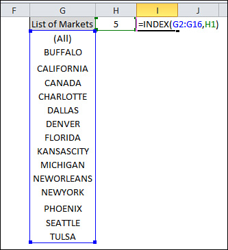
An INDEX function requires two arguments to work properly. The first argument is the range of the list you are working with. In most cases, you use the same range that is feeding your combo box. The second argument is the index number. If the index number is in a cell such as cell H1, you can simply reference the cell.
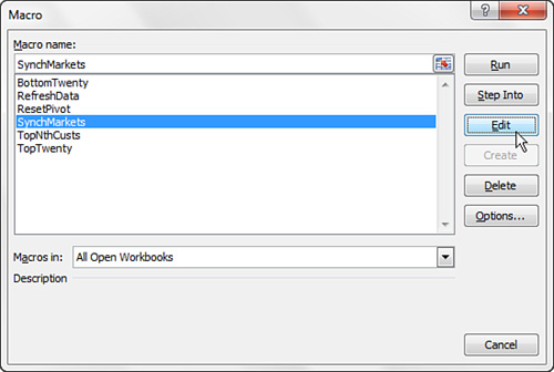
6. Edit the SynchMarkets macro using the value in cell I1, instead of a hard-coded value. To get to the VBA code that makes up your macro, click the Macros button on the Developer tab. This activates the Macro dialog box, as shown in Figure 11.20. From here, select the SynchMarkets macro, and then select Edit.
Figure 11.20 In the Macro dialog box, select the SynchMarkets macro, and then select Edit.
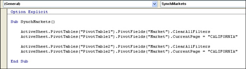
When you recorded your macro originally, you selected the California market from the Market field in both pivot tables. As you can see in Figure 11.21, California is hard-coded in your macro’s VBA code.
Figure 11.21 The California market is hard-coded in your macro’s VBA code.
Replace California with ActiveSheet.Range("I1").Value, as demonstrated in Figure 11.22. This code references the value in cell I1. After you have edited the macro, close the Visual Basic Editor to get back to the spreadsheet.
Figure 11.22 Replace California with a pointer to Range I1 and then close the Visual Basic Editor.

7. All that is left to do is ensure that the macro plays when you select a market from the combo box. Right-click the combo box, and then select Assign Macro. Select the SynchMarkets macro, and then click OK.
8. Clean up the formatting on your newly created report by hiding the rows and columns that hold the filter fields in your pivot tables, the market list you created, and any unseemly formulas.
As you can see in Figure 11.23, this setup provides your clients with an attractive interface that enables them to make selections in multiple pivot tables using one control.
Figure 11.23 Your pivot table report is ready to use!
Tip
When you select a new item from your combo box, the pivot tables automatically adjust the columns to fit the data. This behavior can be annoying when you have a formatted template. You can suppress this behavior by right-clicking on each pivot table, and then selecting Table Options. Selecting this option activates the PivotTable Options dialog box, where you can clear the Autofit Column Widths check box on Update selection.
Next Steps
In the next chapter, you go beyond recording macros. Chapter 12, “Using VBA to Create Pivot Tables,” shows how to utilize VBA to create powerful, behind-the-scenes processes and calculations using pivot tables.