8. Sharing Pivot Tables with Others
As pivot tables evolved in Excel 2007 and Excel 2010, certain incompatibilities were introduced when you share your pivot table with people using legacy versions of Office.
Office 2003 had offered a way to share pivot tables with interactivity to a web page using Office Web Services. This ability was removed in Excel 2007 and is now replaced in Excel 2010 using the Excel Web Application. The Excel Web Application offers interactivity with slicers. The Excel Web Application is actually a hosted version of the Excel Services functionality introduced in Excel 2007 for people using SharePoint.
Sharing a Pivot Table with Other Versions of Office
A version property is attached to every pivot table. This property controls certain behaviors for compatibility with previous versions of Excel.
New pivot tables created in Excel 2010 have a version number of 14, whereas pivot tables created in Excel 2007 have a version number of 12. Pivot tables that were created originally in Excel 2002 or 2003 have a version number of 10. This section explains the compatibility issues you encounter when opening a pivot table created with a different version of Excel.
Compatibility Issues Between Excel 2007 and Excel 2010
You should be thrilled that Microsoft continues to invest heavily in pivot tables. The downside of this investment is that pivot tables created in Excel 2010 will not play well with people who are using Excel 2007. Several issues are explained here.
Slicers Disappear in Excel 2007
Slicers were not available in Excel 2007. For this reason, if you create a slicer in Excel 2010, and then open that workbook in Excel 2007, a box appears where the slicer used to be. The box indicates that this shape represents a slicer created in a newer version of Excel and cannot be used in this version.
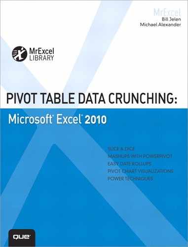
However, the problem is a bit more insidious. In Figure 8.1, a slicer in an Excel 2010 pivot table limits the pivot table to only the East region. Sales are $2.4 million.
Figure 8.1 An Excel 2010 pivot table uses a slicer to show only the East region.
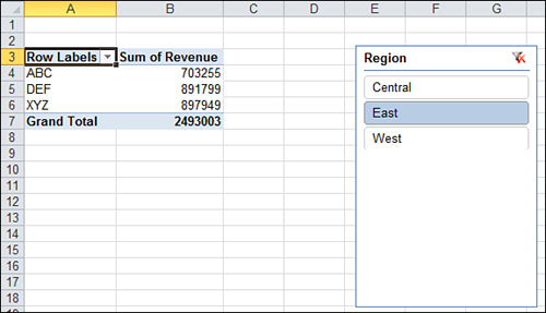
If someone opens the workbook in Excel 2007, an Excel Shape object appears where the slicer used to be. The shape warns that slicers cannot be used in this version of Excel. However, because you were using the slicer to filter instead of using the Report Filter, there is no visible reason to explain why sales are only $2.4 million (see Figure 8.2).
Figure 8.2 When opened in Excel 2007, the slicer is gone. Someone might mistakenly assume the total revenue was only $2.4 million.
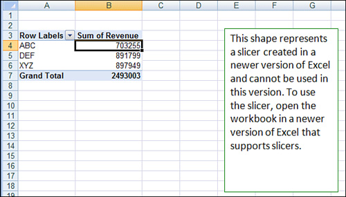
If the person using Excel 2007 refreshes the pivot table, they see the Grand Total changes without any apparent reason (see Figure 8.3). The underlying reason is that the filter applied through the slicer is no longer stored in the pivot table.
Figure 8.3 After a refresh, the revenue changes for no apparent reason.
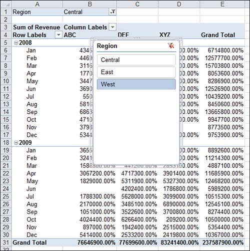
In another example, say you build a pivot table in Excel 2010. You add a slicer for Region and move the region field to the Report Filter. You also limit the report to the West region. Save the file in Excel 2010. Open it in Excel 2007. Change the Report Filter from the West region to the Central region. If you save the file in Excel 2007 and then open it in Excel 2010, the slicer returns, but the file is corrupt. The slicer says West, but the filter says Central, and the actual numbers in the table show all regions (see Figure 8.4).
Figure 8.4 If you round-trip this pivot table from 2010 to 2007 and then back to 2010, the slicer remains, but the file is corrupt.
Percent of Parent Item Calculations Will Not Refresh
Certain calculations in the Show Values As were not available in previous versions of Excel. For example, if you use % of Parent Item, Rank, or % Running Total, the pivot table opens in Excel 2007 and even shows the results. However, the field setting in 2007 indicates that the calculation should be Normal. This means that any change to the pivot table causes the pivot table to begin showing the value field as Normal instead of the correct setting.
Repeat All Labels Is Lost After Any Change in 2007
Repeat All Item Labels on the Report Layout is not available in Excel 2007. An Excel 2010 pivot table with this setting initially appears with the item labels repeated. After any change to the pivot table, the repeated items labels disappear and the setting is lost when you return to Excel 2010.
Excel 2007 Pivot Tables Work Fine in Excel 2010
If you create a pivot table in Excel 2007 and then open it in Excel 2010, you should find no limitations. In addition, you can add Excel 2010 features to pivot tables created in Excel 2007.
Features Unavailable When a Legacy Pivot Table Is Opened in Excel 2010
If you open a pivot table created in Excel 2003 in Excel 2010, the following features are not available:
• Label filtering is grayed out. For example, this is the menu item where you can choose all customers whose names start with A.
• Most Value filtering is unavailable. The only exception is the Top 10 filter.
• Manual Inclusive filtering is unavailable.
• Slicers are unavailable.
• Certain items in the Show Values As menu are unavailable. These include % of Parent, % Running Total In, and Rank options.
• Formatting of hidden items is unavailable. In Excel 2010, if you format a field, remove the field from the table, and then later add it back to the table, the format is remembered. This functionality is not present in Excel 2003 version 10 pivot tables.
• The capability to hide intermediate levels of hierarchies in OLAP data sources is not available.
• The use of key performance indicators from a SQL Server Analysis Services data set is disabled.
• The number of rows is limited to 64,000 instead of 1 million.
• The number of columns is limited to 255 instead of 16,000.
• The maximum number of unique items in a pivot table is limited to 32,000 instead of 1 million.
• Field labels are truncated after 255 characters instead of 32,000 characters.
• The number of fields in the field list is limited to 255 instead of 16,000.
Excel 2010 Compatibility Mode
To a certain extent, version number is controlled in Excel 2010 by compatibility mode. If you create a new pivot table in a workbook that is still in compatibility mode, the pivot table is created as a version 10 pivot table.
When you save the workbook from compatibility mode to one of the new file formats, all the pivot tables are marked for upgrade. You must go through and refresh each pivot table to convert the pivot table to a version 14 pivot table.
No Downgrade Path Available from Version 12 and Version 14 Pivot Tables
After a pivot table has been upgraded to version 12 or 14, it no longer functions in legacy versions of Excel. Even if you save the file in compatibility mode, the pivot table is no longer refreshable.
Strategies for Sharing Pivot Tables
Version 12 and 14 pivot tables cannot be refreshed by anyone using legacy versions of Excel. Therefore, if you want to share a pivot table with someone using a legacy version of Excel, you must take extra care to make sure that the pivot table never existed as a version 12 or 14 pivot table.
You can follow these steps to create a version 10 pivot table:
1. Open a new Excel workbook.
2. Save the workbook as Excel 97–2003 format. Close and reopen the workbook.
3. Copy and paste your data set from the Excel 2010 workbook to the Excel 2003 workbook.
4. Create the pivot table in the Excel 2003 workbook while in compatibility mode.
Saving Pivot Tables to the Web
Unless you had an expensive SharePoint configuration, there was no way to interact with pivot tables in a browser using Excel 2007. It is slick that the new Excel 2010 Web Application will render slicers and pivot tables, but this still does not offer all the interactivity that used to be available in Excel 2003’s Save As Webpage command.
Using Web Services in Excel 2003
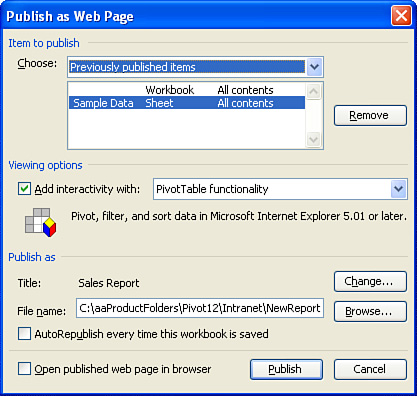
The interactivity available in Excel 2003 might be a reason to keep one computer in the office that still has Excel 2003 installed. In Excel 2003, you would select File, Save As Web Page, Publish. Specify that the web page should have pivot table functionality, as shown in Figure 8.5.
Figure 8.5 In Excel 2003, you can save the pivot table with pivot table interactivity.
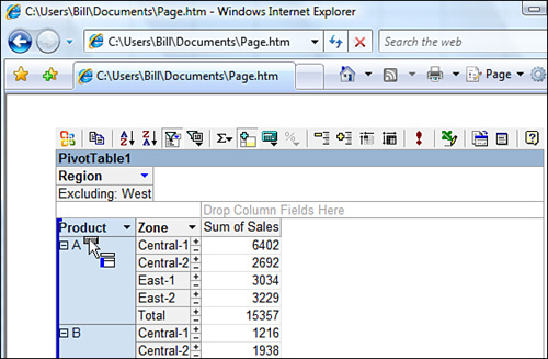
When you open the resulting Web page in a browser, you had an amazing selection of pivot table functionality. You could drag fields to new drop zones. You use the collapse and expand buttons to zoom out or zoom in. You could choose from the report filters. You could even double-click a cell to drill down. The browser version even allowed you to choose multiple items from a Page Filter even though Excel 2003 would not.
Figure 8.6 shows the pivot table rendered in a browser.
Figure 8.6 When opened in Internet Explorer, the Web page offered pivot table functionality when using Excel 2003.
Using Save As HTML in Excel 2010 Provides a Static Image
You can still use File, Save As, HTML to save the workbook as an HTML page. Microsoft quit investing in this technology after Excel 2003. The Save With Interactivity feature is gone. You will get a static view of your pivot table rendered as a report in the browser. There will be no slicers, no charts, no graphics.
Follow these steps to create a static image of the pivot table:
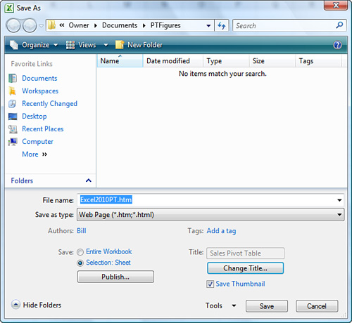
1. From the File menu, select Save As.
2. In the Save as Type drop-down, select Web Page.
3. Click the Publish button to display the Publish as Web Page dialog box, as shown in Figure 8.7.
Figure 8.7 In the Publish as Web Page dialog box, you can specify a few options for the Web page.
4. Click the Title button to specify a title for the Web page.
5. If you want the Web page updated every time the file is saved, select the AutoRepublish check box.
6. Specify a filename for the resulting Web page.
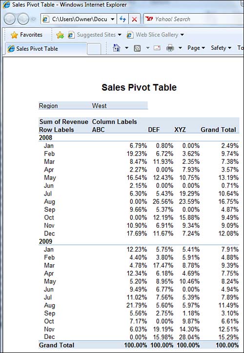
7. Click Publish. Excel writes out a static view of the Web page, as shown in Figure 8.8.
Figure 8.8 The resulting Web page is a static view of the data.
Publishing Pivot Tables to Excel Services in Excel 2010
Starting in Excel 2007, Microsoft revealed their replacement for Office Web Services. The Excel Services product in Excel 2007 required an expensive SharePoint installation.
Excel services supports loading, calculating, and rendering Excel spreadsheets on servers. The person reading the Excel spreadsheet can access the file through his browser.
As the author of the file, you can specify certain cells that the end user can change in the browser. These fields can even be filter fields in your pivot table. Imagine the possibilities for creating fantastic ad hoc reporting tools that people can use to query your data.
Even better, if your Excel spreadsheet is querying an SQL Server database, every time the browser is refreshed, the Excel file pulls new data from the SQL Server, providing real-time business intelligence.
There are three likely scenarios when you want to use Office Services:
• Allow everyone to have read-only access to a single version of an important spreadsheet. This eliminates the problem of multiple versions of the spreadsheet floating around.
• Encapsulate several ranges of various spreadsheets into an executive dashboard running in a browser.
• Build a custom application in the browser that reuses logic already designed in the Excel spreadsheet.
Requirements to Render Spreadsheets with Excel Services
The requirements for Excel Services are fairly high-end. Your organization needs to provide a server running Windows Server 2008R2. You need the Enterprise Editions of SharePoint Server and Excel Services for SharePoint.
As the author of the spreadsheet, you need read-write access to the server.
Preparing Your Spreadsheet for Excel Services
You need to decide carefully which cells in your spreadsheet can be edited by the end user. In a pivot table spreadsheet, these fields are likely the value fields in the Report Filter section of the report.
You need to assign each of these cells a name. To assign a name, follow these steps:
1. Select the desired cell.
2. To the left of the formula bar is the Name box. Typically, this box shows the cell address, such as A1. Click in this box and type a name for the cell. Do not use spaces in the name. “WhichYear” or “Which_Year” are valid. “Which Year” is not valid.
3. Press the Enter key to accept the name.
If you need to later change or delete a name, use the Name Manager icon on the Formulas tab.
Publishing Your Spreadsheet to Excel Services
The first time you publish your spreadsheet, you have to go through a few extra steps to specify the parameter cells. Make sure you have assigned range names to the parameter cells before starting this process. Then do the following:
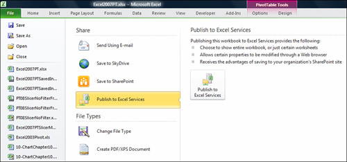
1. From the File menu, select Share, and then Publish to Excel Services, as shown in Figure 8.9.
Figure 8.9 Access Excel Services through the Share category in the File menu.
2. Specify a path and filename in the Save As dialog box.
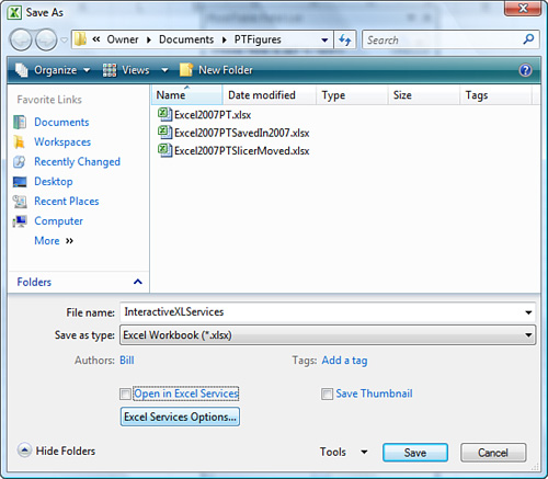
3. If this is the first time you are publishing the workbook, click the Excel Services Options button, as shown in Figure 8.10. Excel displays the Excel Services Options dialog box.
Figure 8.10 Click the Excel Services Options button to access the parameter selection.
4. There are two tabs in the Excel Services Options dialog box. On the Show tab, choose which spreadsheet(s) you want to include in the browser.
5. Click the Parameters tab. Click the Add button to display the Add Parameters dialog box.
6. On the Add Parameters dialog box, you see a list of all named ranges in the worksheet. Click the ranges that you want to specify as parameters (see Figure 8.11).
Figure 8.11 On the Add Parameters dialog box, choose which named ranges to use as parameters.

7. Click OK to close the Add Parameters dialog box.
8. Click OK to close the Excel Services Options dialog box.
9. Click Save to save the worksheet for Excel Services.
What the End User Sees in Excel Services
The goals of Excel Services are:
• Enable the end user to view data in the spreadsheet
• Navigate around the spreadsheet
• Perform further exploration of the data in the spreadsheet
• Change parameters to facilitate what-if analysis
Microsoft has enabled a limited subset of features that allow the end user to achieve these four goals.
Excel Services is not designed to enable someone to author a new spreadsheet. To do this, the user would need to own Excel 2010. Instead, Excel Services allows:
• Support for basic Excel formatting (row height, column width, font, color, gridlines, text rotation). Excel Services also supports data bars, color scales, and table style formatting.
• Capability to switch between sheets in the workbook.
• Support for the use of expand and collapse buttons, either in pivot tables or when using the group and outline buttons.
• Support for querying external data and refreshing that data.
• Support for the Find utility.
• Support for displaying charts.
• Support for filtering and sorting within a defined table.
• Support for filtering and sorting within a pivot table.
As the author of the worksheet, you have a certain amount of control in this support. For example, you can specify that you do not want interactivity to be enabled for the spreadsheet.
Note
One difference between Excel and Excel Services is that Excel Services creates sections of the worksheet and serves up only one section at a time. A typical section contains 75 rows and 20 columns. This is primarily a performance consideration; you do not want the browser attempting to render 20 million cells at once.
What You Cannot Do with Excel Services
Although Excel Services handles many aspects of Excel files, it does not support several features. Any of the items discussed in this section causes the Excel workbook not to load in Excel Services:
• Spreadsheets with code. This includes spreadsheets with VBA macros, forms controls, toolbox controls, Microsoft Excel 5.0 dialog boxes, and XLM sheets.
• IRM-protected spreadsheets
• ActiveX controls
• Embedded SmartTags
• Pivot tables based on “multiple consolidation” ranges
• External references (links to other spreadsheets)
• Spreadsheets saved in formula view
• XML expansion packs
• XML maps
• Data validation
• Query tables, SharePoint lists, Web queries, and text queries
• Spreadsheets that reference add-ins
• Spreadsheets that use the RTD() function
• Spreadsheets that use spreadsheet and sheet protection
• Embedded pictures or clip art
• Cell and Sheet background pictures
• AutoShapes and WordArt
• Ink annotations
• Organization charts and diagrams
• DDE links
Other items are not displayed by Excel Services. For example, if a worksheet contains items in the following list, the worksheet is still displayed, but the item in question is ignored:
• Split and freeze panes
• Headers and footers
• Page layout view
• Cell patterns
• Zoom
• Analysis Services’ member properties in ToolTips
• Some cell formatting (for example, diagonal borders and border types are not supported by HTML)
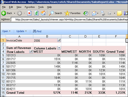
Viewing the Pivot Table in the Browser
After publishing the file to Excel Services, you can open the workbook with Internet Explorer or Firefox. Navigation aids in the browser include the following:
• Sheet tabs in the lower-left corner
• Filter button to control the pivot table filter fields in Cell B1
• Drop-down in Cell B3
Tip
The report in Figure 8.12 still looks like a spreadsheet. If you are trying to use spreadsheet logic in a quick application, you might want to turn off gridlines and row and column headers in the original workbook before publishing to Excel Services.
Figure 8.12 This Web page has a surprising amount of spreadsheet-like functionality.
Viewing Your Excel 2010 Pivot Table on the SkyDrive
The new Excel Web App in Excel 2010 will allow you to save a pivot table complete with slicers and charts to the Windows Live SkyDrive. You can view the pivot table in the browser, interact with the slicers, and see the pivot table and pivot charts update.
On the one hand, rendering of charts and slicers is a tremendous improvement over the options available in Excel 2003. On the other hand, the Excel 2003 interactivity would allow you to drag fields around the pivot table. The Excel 2010 web application is not there yet.
To access the SkyDrive, you need to sign up for a free account in Live.com.
Once you are signed in to the SkyDrive, open the More drop-down and choose SkyDrive.
By default, the My Documents folder is a private folder. You can create new folders on the SkyDrive and either make these public or share them with a specific list of Windows Live accounts.
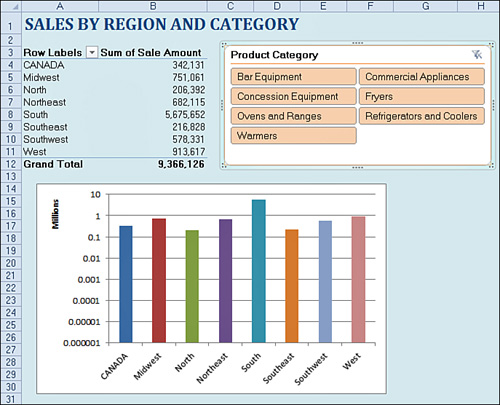
Figure 8.13 shows a worksheet in Excel 2010. A pivot table in A3:A12 summarizes 6000 rows of data. One slicer controls the pivot table and the chart is based on the results of the pivot table.
Figure 8.13 This workbook in Excel 2010 includes a pivot table, slicers, and a chart.
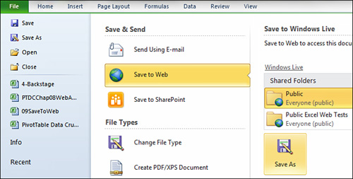
Choose File, Share, Save to Web. Sign in to your SkyDrive account and then use the Save As button to save the workbook on your SkyDrive (see Figure 8.14).
Figure 8.14 Choose to save to your SkyDrive.
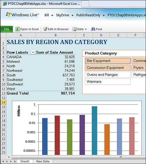
In the SkyDrive, choose View. The pivot table, the slicers, and the chart all render in the browser. You can select new categories from the slicer. The pivot table and the chart all render in a few seconds. This is an impressive dashboard created using Excel 2010. (see Figure 8.15).
Figure 8.15 This workbook, complete with working slicers, is rendered in a browser with no need for Excel on the computer.
Tip
If you have saved the workbook in a public folder, you can share it by sharing the URL from the address bar.
![]() To see a demo of saving a pivot table to the Excel Web App, search for “Pivot Table Data Crunching 8” at YouTube.
To see a demo of saving a pivot table to the Excel Web App, search for “Pivot Table Data Crunching 8” at YouTube.
The Row Labels dropdown in cell A3 of Figure 8.15 offers choices to let you sort the regions by region name or the sales value.
Although the Excel Web App will let you edit the worksheet in the browser, you can not create a new pivot table nor rearrange fields in the Excel Web App.
Next Steps
In the next chapter, you learn about running pivot tables on data stored outside Excel including OLAP data sources and SQL Server.