7. Analyzing Disparate Data Sources with Pivot Tables
Until this point, you have been working with one local table located in the worksheet within which you are operating. Indeed, it would be wonderful if every data set you came across were neatly packed in one easy-to-use Excel table. Unfortunately, the business of data analysis does not always work out that way.
The reality is that some of the data you encounter comes from disparate data sources—meaning sets of data that are from separate systems, stored in different locations, or saved in a variety of formats. In an Excel environment, disparate data sources generally fall into one of two categories: external data and multiple ranges.
External data is exactly what it sounds like—data that is not located in the Excel workbook in which you are operating. Some examples of external data sources are text files, Access tables, SQL Server tables, and other Excel workbooks.
Multiple ranges are separate data sets located in the same workbook but separated either by blank cells or by different worksheets. For example, if your workbook has three tables on three different worksheets, each of your data sets covers a range of cells. You are therefore working with multiple ranges.
A pivot table can be an effective tool when you need to summarize data that is not neatly packed into one table. With a pivot table, you can quickly bring together either data found in an external source or data found in multiple tables within your workbook. In this chapter, you discover how to work with external data sources and data sets located in multiple ranges within your workbook.
Using Multiple Consolidation Ranges
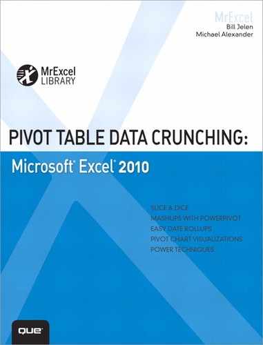
If you need to analyze data dispersed in multiple ranges, your options are somewhat limited. For example, the data in Figure 7.1 shows you three ranges that you need to bring together to analyze as a group.
Figure 7.1 Someone passed you a file that has three ranges of data. You need to bring the three ranges together so you can analyze them as a group.
You essentially have three paths you can take to get to the point where you can analyze all three ranges together:
• You can obtain the original data used to create this summary. This seems like a good choice, but in most cases, you could find another solution by the time it took you to obtain the original data—if you have access to it at all.
• You can manually shape the data into a proper tabular data set and then do your analysis. In reality, this option would be the best one if you had the time to spare or you were planning to use this data on an ongoing basis. However, if this is a one-time analysis or if you’re in a crunch, you would not want to spend the time to manually format this data.
• You can create a pivot table using multiple consolidation ranges. With this pivot table option, you can quickly and easily consolidate all the data from your selected ranges into a single pivot table. This is the best option if you need to perform only a one-time analysis on multiple ranges or if you need to analyze multiple ranges in a hurry.
To start the process of bringing this data together with a pivot table, you have to activate the classic PivotTable and PivotChart Wizard.
Activating the Classic PivotTable and PivotChart Wizard
As you learned in Chapter 2, “Creating a Basic Pivot Table,” Microsoft has abandoned the classic PivotTable and PivotChart Wizard for a streamlined dialog box. Unfortunately, some of the functionality exposed in the classic wizard was not brought over with the new pivot table interfaces. The capability to create multiple consolidation range pivot tables is one example of functionality that did not make its way to Excel’s new UI.
The good news is that Excel does enable you to activate the classic wizard (complete with all the old functionality) through a custom toolbar command. The idea is to add the PivotTable and PivotChart Wizard custom toolbar command to the Quick Access toolbar. After it’s on the Quick Access toolbar, you can call up the classic wizard simply by clicking on the icon.
Follow these steps to add the PivotTable and PivotChart Wizard custom toolbar command to the Quick Access toolbar:
1. Click the File tab on the Ribbon.
2. Select Options to open the Options dialog box.
3. Select Quick Access Toolbar to bring up all the available commands that can be added to the Quick Access toolbar.
4. In the Choose Commands From drop-down box, select Commands Not in the Ribbon.
5. Select the PivotTable and PivotChart Wizard from the list of commands and click the Add button.
6. Click OK.
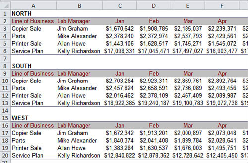
As you can see in Figure 7.2, your reward is an easily accessible icon that calls the classic PivotTable and PivotChart Wizard.
Figure 7.2 Add the PivotTable and PivotChart Wizard command to the Quick Access toolbar.
Tip
You can also activate the classic PivotTable and PivotChart Wizard by pressing Alt+D+P on your keyboard. Keep in mind this approach does not add an icon to the Quick Access toolbar.
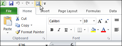
After you have access to the PivotTable and PivotChart Wizard, activate it and then select Multiple Consolidation Ranges, as demonstrated in Figure 7.3. Then, select Next.
Figure 7.3 Start the PivotTable and PivotChart Wizard and select Multiple Consolidation Ranges. Select Next to move to the next step.
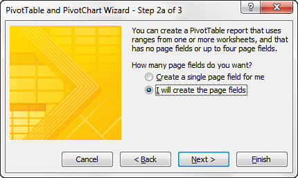
In the next step, you specify if you want Excel to create one page field for you or if you would like to create your own. In most cases, the page fields that Excel creates are ambiguous and of no value. Therefore, in almost all cases, you should select the option of creating your own page fields, as illustrated in Figure 7.4. Then, select Next.
Figure 7.4 Specify that you want to create your own page fields, and then select Next.
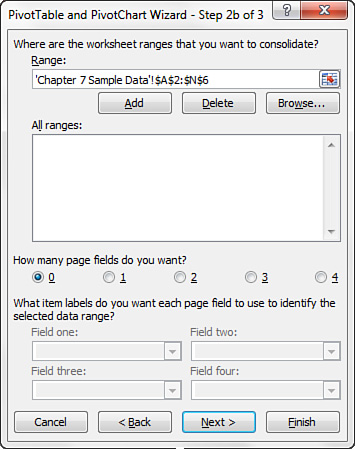
Next, you need to point Excel to each of your individual data sets one by one. Simply select the entire range of your first data set and select Add, as shown in Figure 7.5.
Figure 7.5 Select the entire range of your first data set and select Add.
Caution
For your pivot table to generate properly, the first line of each range must include column labels.
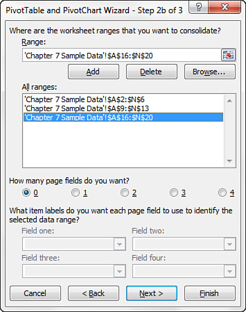
Select the rest of your ranges and add them to your list of ranges. At this point, your dialog box should look similar to the one in Figure 7.6.
Figure 7.6 Add the other two data set ranges to your range list.
Notice that each of your data sets belongs to a Region (North, South, or West). When your pivot table brings your three data sets together, you need a way to parse out each Region again.
To ensure you have that capability, you need to tag each range in your list of ranges with a name identifying which data set that range came from. The result is the creation of a Page field that enables you to filter each region as needed.
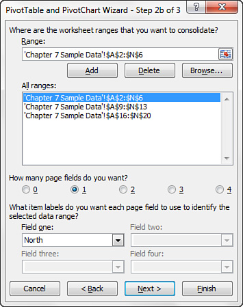
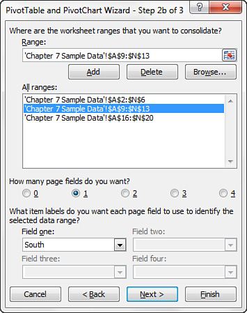
The first thing you have to do to create your Region page field is specify how many page fields you want to create. In your case, you want to create only one page field for your region identifier, so simply click the radio button next to the number 1, as demonstrated in Figure 7.7. This action enables the Field One input box. As you can see, you can create up to four page fields.
Figure 7.7 To be able to filter by Region when your pivot table is complete, you have to create a page field. Click the radio button next to the number 1 to create one page field. This action enables the Field One input box.

You have to tag each range one by one, so click the first range in your range list to highlight it. Enter the region name into the Field One input box. As you can see in Figure 7.8, the first range is made up of data from the North region, so you enter North in the input box.
Figure 7.8 Select the first range that represents the data set for the North region and enter the word North in the input box.
Repeat the process for the other regions, as illustrated in Figure 7.9. When you’re done, select Next.
Figure 7.9 Repeat the process until you have tagged all your data sets. When you’re done, select Next.
The last step is to choose the destination of your new pivot table. In this case, select the New worksheet option, and then click Finish.
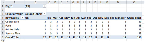
You have successfully brought three data sources together into one pivot table, as shown in Figure 7.10.
Figure 7.10 You now have a pivot table that contains data from three data sources.
Analyzing the Anatomy of a Multiple Consolidation Range Pivot Table
Take a moment to analyze your new pivot table. You might notice a few interesting things. First, your field list includes a field called Row, a field called Column, a field called Value, and a field called Page1.
It is important to keep in mind that pivot tables using multiple consolidation ranges as their data source can have only three base fields: Row, Column, and Value. In addition to these base fields, you can create up to four page fields.
Tip
Notice that the fields generated with your pivot table have fairly generic names (Row, Column, Value, and Page). You can customize the field settings for these fields to rename and format them to better suit your needs.
→ See Chapter 3, “Customizing a Pivot Table,” for a more detailed look at customizing field settings.
The Row Field
The Row field is always made up of the first column in your data source. Note that in Figure 7.1, the first column in your data source is Line of Business. Therefore, the Row field in your newly created pivot table contains Line of Business.
The Column Field
The Column field contains the remaining columns in your data source. Pivot tables that use multiple consolidation ranges combine all the fields in your original data sets (minus the first column, which is used for the Row field) into a kind of super field called the Column field. The fields in your original data sets become data items under the Column field.
Notice that your pivot table initially applies Count to your Column field. If you change the field setting of the Column field to Sum, all the data items under the Column field are affected. Figure 7.11 shows the same data as Figure 7.10, except the summarize type is set to Sum instead of the default Count.
Figure 7.11 The data items under the Column field are treated as one entity. When you change the calculation of the Column field from Count to Sum, the change applies to all items under the Column field.
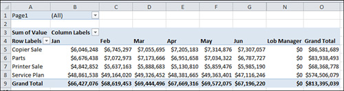
The Value Field
The Value field contains the value for all data items under the Column field. Notice that even fields that were originally text fields in your data set are treated as numerical values. An example is Lob Manager in Column N, which is shown in Figure 7.11. Although this field contained manager names in the original data set, it is now treated as a number in your pivot table.
As mentioned before, pivot tables that use multiple consolidation ranges merge the fields in your original data sets (minus the first field), making them data items in the Column field. Although you might recognize fields like Lob Manager as text fields that contain their own individual data items, they no longer hold data of their own. They have been transformed into data items themselves—data items with a value.
The net effect of this behavior is that fields originally holding text or dates show up in your pivot table as a meaningless numerical value. It’s usually a good idea to simply hide these fields to avoid confusion.
→ See Chapter 3, “Customizing a Pivot Table,” for a more detailed look at customizing field settings.
The Page Fields
Page fields are the only fields in multiple consolidation range pivot tables that you have direct control over. You can create and define up to four page fields. The useful feature of these fields is that you can drag them to the row area or column area to add layers to your pivot table.
The Page1 field shown in the pivot table in Figure 7.11 was created to filter by region. However, if you move the Page1 field to the row area of your pivot table, you can create a one-shot view of all your data by region. Figure 7.12 demonstrates this view.
Figure 7.12 Moving the Page1 field to the row area adds a layer to your pivot table report, giving you a one-shot view of all your data by region.

Tip
Your pivot table might have a different layout than Figure 7.12. You can achieve the same layout by selecting Design from the PivotTable Tools tab, and then selecting Report Layout in the Layout group. Then, you can select Show in Tabular Form to get the same layout.
Redefining Your Pivot Table
You might run into a situation in which you need to redefine your pivot table. That is, you need to add a data range, remove a data range, or redefine your page fields. To redefine your pivot table, simply activate the classic PivotTable and PivotChart Wizard, and then select the Back button until you get to the dialog box you need.
Building a Pivot Table Using External Data Sources
There is no argument that Excel is good at processing and analyzing data. In fact, pivot tables themselves are a testament to the analytical power of Excel. However, despite all its strengths, Excel makes for a poor data management platform, primarily for three reasons:
• A data set’s size has a significant impact on performance, making for less efficient data crunching. The reason for this is the fundamental way Excel handles memory. When you open an Excel file, the entire file is loaded into RAM to ensure quick data processing and access. The drawback to this behavior is that Excel requires a great deal of RAM to process even the smallest change in your spreadsheet (typically giving you a “Calculating” indicator in the status bar). So although Excel 2010 offers over 1 million rows and over 16,000 columns, creating and managing large data sets causes Excel to slow down considerably, making data analysis a painful endeavor.
• The lack of a relational data structure forces the use of flat tables that promote redundant data. It also increases the chance for errors.
• There is no way to index data fields in Excel to optimize performance when you’re attempting to retrieve large amounts of data.
In smart organizations, the task of data management is not performed by Excel; rather, it is primarily performed by relational database systems such as Microsoft Access and SQL Server. These databases are used to store millions of records that can be rapidly searched and retrieved.
The effect of this separation in tasks is that you have a data management layer (your database) and a presentation layer (Excel). The trick is to find the best way to get information from your data management layer to your presentation layer for use by your pivot table.
Managing your data is the general idea behind building your pivot table using an external data source. Building your pivot tables from external systems enables you to leverage environments that are better suited to data management. This means you can let Excel do what it does best: analyze and create a presentation layer for your data. The following sections walk you through several techniques that enable you to build pivot tables using external data.
Building a Pivot Table with Microsoft Access Data
Often Access is used to manage a series of tables that interact with each other, such as a Customers table, an Orders table, and an Invoices table. Managing data in Access provides the benefit of a relational database where you can ensure data integrity, prevent redundancy, and easily generate data sets via queries.
The modus operandi of most Excel users is to use an Access query to create a subset of data and then import that data into Excel. From there, the data can be analyzed with pivot tables. The problem with this method is that it forces the Excel workbook to hold two copies of the imported data sets: one on the spreadsheet and one in the pivot cache. Holding two copies obviously causes the workbook to be twice as big as it needs to be, and it introduces the possibility of performance issues.
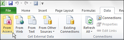
Excel 2010 offers a surprisingly easy way to use your Access data without creating two copies of your data. To see how easy it is, open Excel and start a new workbook. Then, click the Data tab and look for the group called Get External Data. Here, you find the From Access selection, as shown in Figure 7.19.
Figure 7.19 Click the From Access button to get data from your Access database.
Tip
The sample database used in this chapter is available for download from www.MrExcel.com/pivotbookdata2010.html.
Selecting the From Access button activates a dialog box asking you to select the database you want to work with. Select your database.
After your database has been selected, the dialog box shown in Figure 7.20 activates. This dialog box lists all the tables and queries available. In this example, select the query called Sales_By_Employee and click OK.
Figure 7.20 Select the table or query you want to analyze.
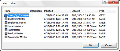
Note
In Figure 7.20, notice that the Select Table dialog box contains a column called Type. There are two types of Access objects you can work with: Views and Tables. View indicates that the data set listed is an Access query, and Table indicates that the data set is an Access table.
In this example, notice that Sales_By_Employee is actually an Access query. This means that you import the results of the query. This is true interaction at work; Access does all the backend data management and aggregation, and Excel handles the analysis and presentation!
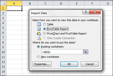
Next, you see the Import Data dialog box, where you select the format in which you want to import the data. As you can see in Figure 7.21, you have the option of importing the data as a table, as a pivot table, or as a pivot chart with an accompanying pivot table. You also have the option to tell Excel where to place the data.
Figure 7.21 Select the radio button next to PivotTable Report.
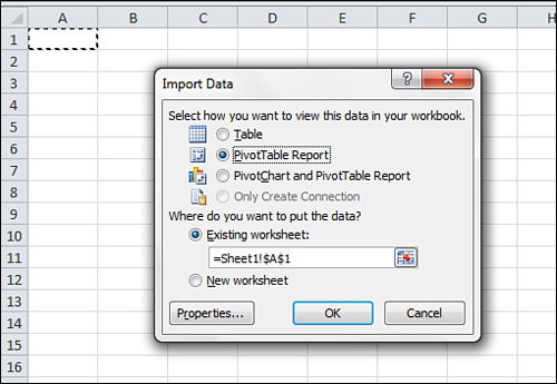
Select the radio button next to PivotTable Report and click OK.
At this point, you should see the PivotTable Field List shown in Figure 7.22. From here, you can use this pivot table just as you normally would.
Figure 7.22 Your pivot table is ready to use.
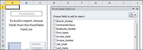
The wonderful thing about this technique is that the only copy of the data resides inside the pivot cache. You won’t find the data in any of the other tabs. Does this present a problem when you need to get to the raw data in the pivot cache? The answer is no.
You can tell the pivot cache to output a raw data set for any dimension in the pivot table simply by double-clicking on the data for that dimension. For example, Figure 7.23 illustrates how double-clicking the Grand Total for Mr. Gall outputs all the raw records that make up his Grand Total. The output is automatically placed into a separate tab.
Figure 7.23 Double-clicking on the totals in the data area of a pivot table outputs the raw records that make up that total into a separate tab.

Caution
If you create a pivot table that uses an Access database as its source, you can refresh that pivot table only if the table or view is available. That is, deleting, moving, or renaming the database used to create the pivot table destroys the link to the external data set, thus destroying your ability to refresh the data. Deleting or renaming the source table or query has the same effect.
Following that reasoning, any clients using your linked pivot table cannot refresh the pivot table unless the source is available to them. If you need your clients to be able to refresh, you might want to make the data source available via a shared network directory.
Building a Pivot Table with SQL Server Data
In the spirit of collaboration, Excel 2010 vastly improves your ability to connect to transactional databases such as a SQL Server. With its new connection functionality found in Excel, creating a pivot table from SQL Server data is as easy as ever.
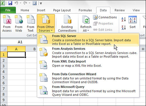
Start on the Data tab and select From Other Sources to see the drop-down menu shown Figure 7.24. Then, select From SQL Server.
Figure 7.24 Select From SQL Server from the drop-down menu.
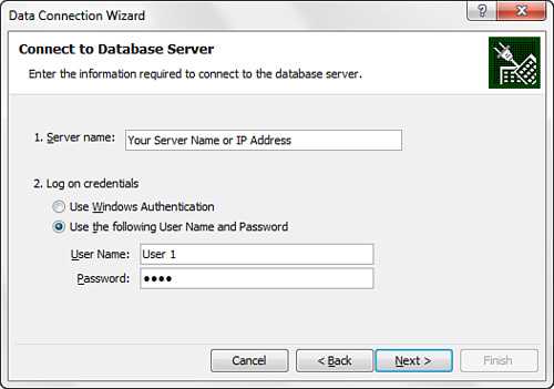
Selecting this option activates the Data Connection Wizard, as shown in Figure 7.25. The idea here is that you configure your connection settings so Excel can establish a link to the server.
Figure 7.25 Enter your authentication information and click Next.
Note
There is no sample file for this case study. The essence of this demonstration is the interaction between Excel and a SQL Server data source. The actions you take to connect to your particular database are the same as demonstrated here.
The first step in this endeavor is to provide Excel with some authentication information. As you can see in Figure 7.25, you enter the name of your server, your username, and your password.
Note
If you are typically authenticated via Windows authentication, you simply select the Use Windows Authentication option.
Next, you select the database with which you are working from a drop-down menu containing all available databases on the specified server. As you can see in Figure 7.26, a database called Facility_Svcs_Database has been selected in the drop-down box. Selecting this database causes all the tables and views in it to be exposed in the list of objects below the drop-down menu. Choose the table or view you want to analyze, and then click Next.
Figure 7.26 Specify your database, and then choose the table or view you want to analyze.

Tip
In Figure 7.26, notice the check box titled Connect to a Specific Table. In most cases, you connect to one table or view that has been created to give you an aggregation or a smaller subset of data for analysis. For this reason, the Connect to aSpecific Table check box is selected by default, enabling you to make only one selection.
If you were to clear the check box, all the objects in the specified database would be selected, giving you access to all the tables and views available. Enabling the selection of all objects in the database enables you to create your own aggregations and queries using MS Query.
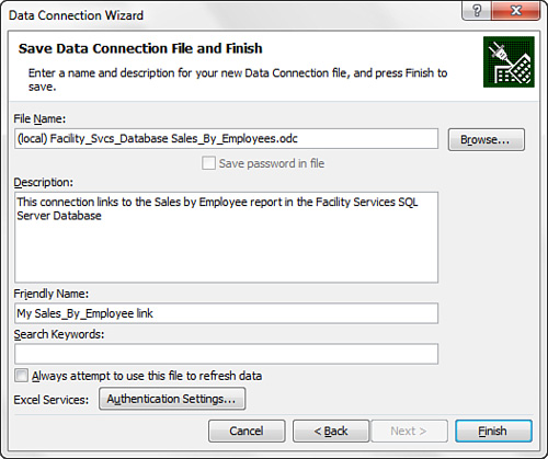
The next screen in the wizard, as shown in Figure 7.27, enables you to enter some descriptive information about the connection you’ve just created.
Figure 7.27 Edit descriptive information for your connection.
Note
All the fields in the screen shown in Figure 7.27 are optional edits only. That is, if you bypass this screen without editing anything, your connection works fine.
The fields that you use most often are:
• File Name—In the File Name input box, you can change the filename of the .odc (Office Data Connection) file generated to store the configuration information for the link you just created.
• Save Password in File—Under the File Name input box, you have the option of saving the password for your external data in the file itself via the Save Password in File check box. Selecting this check box enters your password in the file.
Caution
Keep in mind that this password is not encrypted, so anyone interested enough could potentially get the password for your data source simply by viewing your file with a text editor.
• Description—In the Description field, you can enter a plain description of what this particular data connection does.
• Friendly Name—The Friendly Name field enables you to specify your own name for the external source. You typically enter a name that is descriptive and easy to read.
When you are satisfied with your descriptive edits, click Finish to finalize your connection settings. You immediately see the Import Data dialog box, as shown in Figure 7.28. From here, you select a pivot table, and then click OK to start building your pivot table.
Figure 7.28 When your connection is finalized, you can start building your pivot table.
Next Steps
Chapter 8, “Sharing Pivot Tables with Others,” covers the ins and outs of sharing your pivot tables with the world. You learn how you can distribute your pivot tables to the Web, publish your pivot tables to Excel services, and render your pivot tables through other Microsoft Office applications.