12. Using VBA to Create Pivot Tables

Introducing VBA

Version 5 of Excel introduced a powerful new macro language called Visual Basic for Applications (VBA). Every copy of Excel shipped since 1993 has had a copy of the powerful VBA language hiding behind the worksheets. VBA enables you to perform steps that you normally perform in Excel quickly and flawlessly. I have seen a VBA program change a process that would take days each month and turn it into a single button click and a minute of processing time.

Do not be intimidated by VBA. The VBA macro recorder tool gets you 90 percent of the way to a useful macro, and I get you the rest of the way using examples in this chapter.

Every example in this chapter is available for download from www.mrexcel.com/pivot2010data.html/.

Enabling VBA in Your Copy of Excel

By default, VBA is disabled in Office 2010. Before you can start using VBA, you need to enable macros in the Trust Center. Follow these steps:

1. Click the File menu to show the Backstage View.

2. In the left navigation, select Options. The Excel Options dialog displays.

3. In the left navigation of Excel Options, select Customize Ribbon.

4. The right listbox has a list of main tabs available in Excel. By default, the checkbox for the Developer tab is unchecked. Select this tab to include it in the ribbon. Click OK to close Excel Options.

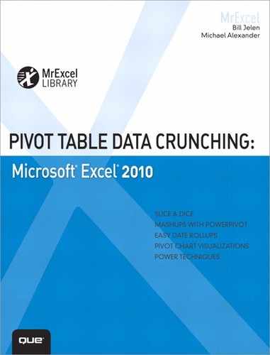
5. Click the Developer tab in the ribbon. As shown in Figure 12.1, the Code group on the left side of the ribbon includes icons for the Visual Basic Editor, Macros, Macro Recorder, and Macro Security.

Figure 12.1 Enable the Developer tab to access the VBA tools.

6. Click the Macro Security icon. Excel opens the Trust Center where you have four security choices. These choices use different words than those used in Excel 97 through Excel 2003. Step 7 explains the choices.

7. Choose one of the following options:

• Disable all macros with notification—This setting is equivalent to medium macro security in Excel 2003. When you open a workbook that contains macros, a message appears alerting you that macros are in the workbook. If you expect macros to be in the workbook, you should click Options, Enable to allow the macros to run. This is the safest setting because it forces you to explicitly enable macros in each workbook.

• Enable all macros—This setting is not recommended because potentially dangerous code can run. However, this setting is equivalent to low macros security in Excel 2003. Because it can enable rogue macros to run in files that are sent to you by others, Microsoft recommends that you do not use this setting.

Using a File Format That Enables Macros

The default Excel 2010 file format is initially the Excel Workbook (.xlsx). This workbook is defined to disallow macros. You can build a macro in a .xlsx workbook, but they will never be allowed to run and won’t be saved with the workbook.

You have several options for saving workbooks that enables macros:

• Excel Macro-Enabled Workbook (.xlsm)—This uses the new xml-based method for storing workbooks and enables macros. I prefer this file type because it is compact and less prone to becoming corrupt.

• Excel Binary Workbook (.xlsb)—This is a binary format and always enables macros.

• Excel 97-2003 Workbook (.xls)—There are billions of .xls files in existence and all of them are capable of storing macros. The downside, particularly with pivot tables, is that .xls files force Excel into compatibility mode. You lose access to Slicers, new Filters, and other pivot table improvements.

When you create a new workbook, you can use File, Save As to choose the appropriate file type.

Visual Basic Editor

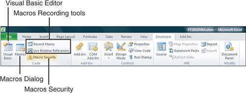
From Excel, press Alt+F11 or select Developer, Visual Basic to open the Visual Basic Editor, as shown in Figure 12.2. The three main sections of the VBA Editor are described here. If this is your first time using VBA, some of these items might be disabled. Follow the instructions given in the following list to make sure that each is enabled.

Figure 12.2 The Visual Basic Editor window is lurking behind every copy of Excel shipped since 1993.

• Project Explorer—This pane displays a hierarchical tree of all open workbooks. Expand the tree to see the worksheets and code modules present in the workbook. If the Project Explorer is not visible, enable it by pressing Ctrl+R.

• Properties window—The Properties window is important when you begin to program user forms. It has some use when you are writing normal code, so enable it by pressing F4.

• Code window—This is the area where you write your code. Code is stored in one or more code modules attached to your workbook. To add a code module to a workbook, select Insert, Module from the VBA menu.

Visual Basic Tools

Visual Basic is a powerful development environment. Although this chapter cannot offer a complete course on VBA, if you are new to VBA, you should take advantage of these important tools:

• As you begin to type code, Excel might offer a drop-down with valid choices. This feature, known as AutoComplete, enables you to type code faster and eliminate typing mistakes.

• For assistance on any keyword, put the cursor in the keyword and press F1. You might need your installation DVDs because the VBA help file can be excluded from the installation of Office 2010.

• Excel checks each line of code as you finish it. Lines in error appear in red. Comments appear in green. You can add a comment by typing a single apostrophe. Use lots of comments so you can remember what each section of code is doing.

• Despite the aforementioned error checking, Excel might still encounter an error at runtime. If this happens, click the Debug button. The line that caused the error is highlighted in yellow. Hover your mouse cursor over any variable to see the current value of the variable.

• When you are in Debug mode, use the Debug menu to step line by line through code. If you have a wide monitor, try arranging the Excel window and the VBA window side by side. This way, you can see the effect of running a line of code on the worksheet.

• Other great debugging tools are breakpoints, the Watch window, the Object Browser, and the Immediate window. Read about these tools in the Excel VBA Help menu.

The Macro Recorder

Excel offers a macro recorder that is about 90 percent perfect. Unfortunately, the last 10 percent is frustrating. Code that you record to work with one data set is hard-coded to work only with that data set. This behavior might work fine if your transactional database occupies Cells A1:L87601 every single day, but if you are pulling in a new invoice register every day, it is unlikely that you will have the same number of rows each day. Given that you might need to work with other data, it would be a lot better if Excel could record selecting cells using the End key. This is one of the shortcomings of the macro recorder.

In reality, Excel pros use the macro recorder to record code but then expect to have to clean up the recorded code.

Understanding Object-Oriented Code

VBA is an object-oriented language. Most lines of VBA code follow the Noun. Verb syntax. However, in VBA, it is called Object.Method. Examples of objects are workbooks, worksheets, cells, or ranges of cells. Methods can be typical Excel actions, such as .Copy, .Paste, and .PasteSpecial.

Many methods allow adverbs—parameters you use to specify how to perform the method. If you see a construct with a := (colon and equal signs), you know that the macro recorder is describing how the method should work.

You also might see the type of code in which you assign a value to the adjectives of an object. In VBA, adjectives are called properties. If you set ActiveCell.Font.ColorIndex = 3, you are setting the font color of the active cell to red. Note that when you are dealing with properties, there is only an = (equal sign), not a := (colon and equal signs).

Learning Tricks of the Trade

You need to master a few simple techniques to write efficient VBA code. These techniques help you make the jump to writing effective code.

Writing Code to Handle Any Size Data Range

The macro recorder hard-codes the fact that your data is in a range, such as A1:L87601. Although this hard-coding works for today’s data set, it might not work as you get new data sets. You need to write code that can deal with different size data sets.

The macro recorder uses syntax such as Range(“H12”) to refer to a cell. However, it is more flexible to use Cells(12, 8) to refer to the cell in Row 12, Column 8. Similarly, the macro recorder refers to a rectangular range as Range(“A1:L87601”). However, it is more flexible to use the Cells syntax to refer to the upper-left corner of the range, and then use the Resize() syntax to refer to the number of rows and columns in the range. The equivalent way to describe the preceding range is Cells(1, 1).Resize(87601,12). This approach is more flexible because you can replace any of the numbers with a variable.

In the Excel user interface, you can use the End key on the keyboard to jump to the end of a range of data. If you move the cell pointer to the final row on the worksheet and press the End key followed by the up-arrow key, the cell pointer jumps to the last row with data. The equivalent of doing this in VBA is to use the following code:

Range("A1048576").End(xlUp).Select

You do not need to select this cell; you just need to find the row number that contains the last row. The following code locates this row and saves the row number to a variable named FinalRow:

FinalRow = Range("A1048576").End(xlUp).Row

There is nothing magic about the variable name FinalRow. You could call this variable x, y, or even your dog’s name. However, because VBA enables you to use meaningful variable names, you should use something such as FinalRow to describe the final row.

You also can find the final column in a data set. If you are relatively sure that the data set begins in Row 1, you can use the End key in combination with the left-arrow key to jump from Cell XFD1 to the last column with data. To generalize for the possibility that the code is running in legacy versions of Excel, you can use the following code:

FinalCol = Cells(1, Columns.Count).End(xlToLeft).Column

Using Super-Variables: Object Variables

In typical programming languages, a variable holds a single value. You might use x = 4 to assign a value of 4 to the variable x.

Think about a single cell in Excel. Many properties describe a cell. A cell might contain a value such as 4, but the cell also has a font size, a font color, a row, a column, possibly a formula, possibly a comment, a list of precedents, and more. It is possible in VBA to create a super-variable that contains all the information about a cell or about any object. A statement to create a typical variable such as x = Range("A1") assigns the current value of A1 to the variable x.

However, you can use the Set keyword to create an object variable:

Set x = Range("A1")

You have now created a super-variable that contains all the properties of the cell. Instead of having a variable with only one value, you have a variable in which you can access the value of many properties associated with that variable. You can reference x. Formula to learn the formula in A1 or x.Font.ColorIndex to learn the color of the cell.

Using With and End With to Shorten Code

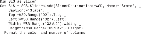
You will frequently find that you are making several changes to the pivot table. Although the following code is explained later in this chapter, all these lines of code are changing settings in the pivot table:

For all those lines of code, the VBA engine has to figure out what you mean by PT. Your code executes faster if you only refer to PT once. Add an initial line of With PT. Then, all the remaining lines do not need to start with PT. Any line that starts with a period is assumed to be referring to the object in the With statement. Finish the code block using an End With statement:

Understanding Versions

Pivot tables have been evolving. They were introduced in Excel 5 and perfected in Excel 97. In Excel 2000, pivot table creation in VBA was dramatically altered. Some new parameters were added in Excel 2002. A few new properties such as PivotFilters and TableStyle2 were added in Excel 2007. Slicers and new choices for Show Values As have been added in Excel 2010. Therefore, you need to be extremely careful when writing code in Excel 2010 that might be run in Excel 2007 or legacy versions of Excel.

New in Excel 2010

Excel 2010 offers many new features in pivot tables. If you use any of these features in VBA, the code works in Excel 2010, but crashes in any previous versions of Excel.

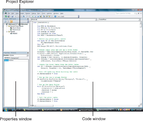
Table 12.1 shows items that are in Excel 2010 VBA for pivot tables. The following items cause incompatibilities when run in Excel 2007.

Table 12.1 Excel 2010 VBA Elements That Are Incompatible with Excel 2007

Concepts Introduced in Excel 2007

If there is some chance that your code runs in Excel 2003, there are even more possible incompatibilities. Many concepts on the Design tab were introduced in Excel 2007, such as subtotals at the top, the report layout options, blank rows, and the new PivotTable styles. Excel 2007 offered better filters than legacy versions. If you are hoping to share your pivot table macro with people running legacy versions of Excel, you need to avoid these methods. Your best bet is to open an Excel 2003 workbook in compatibility mode and record the macro while the workbook is in compatibility mode. If you are using the macro only in Excel 2007 or later, you can use any of these new features.

Table 12.2 shows the methods that were introduced in Excel 2007. If you record a macro that uses these methods, you cannot share the macro with someone using a legacy version of Excel.

Table 12.2 Methods Introduced in Excel 2007

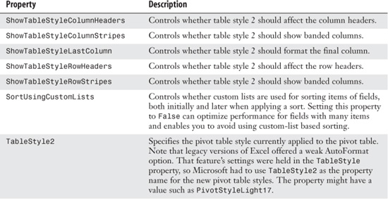
Table 12.3 lists the properties that were new in Excel 2007. If you record a macro that refers to these properties, you cannot share the macro with someone using a legacy version of Excel.

Table 12.3 Properties New in Excel 2010

Building a Pivot Table in Excel VBA

This chapter does not mean to imply that you use VBA to build pivot tables to give to your clients. Instead, the purpose of this chapter is to remind you that pivot tables can be used as a means to an end. You can use a pivot table to extract a summary of data and then use that summary elsewhere.

In Excel 2000 and newer, you first build a pivot cache object to describe the input area of the data:

After defining the pivot cache, use the CreatePivotTable method to create a blank pivot table based on the defined pivot cache:

Set PT = PTCache.CreatePivotTable(TableDestination:=
WSD.Cells(2, FinalCol + 2).TableName:="PivotTable1")

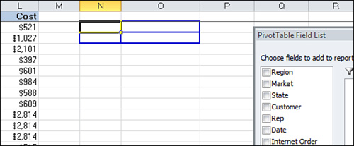
In the CreatePivotTable method, you specify the output location and optionally give the table a name. After running this line of code, you have a strange-looking blank pivot table, like the one shown in Figure 12.3. You now have to use code to drop fields onto the table.

Figure 12.3 Immediately after you use the CreatePivotTable method, Excel gives you a four-cell blank pivot table that is not useful.

If you choose the Defer Layout Update setting in the user interface to build the pivot table, Excel does not recalculate the pivot table after you drop each field onto the table. By default in VBA, Excel calculates the pivot table as you execute each step of building the table. This could require the pivot table to be executed a half-dozen times before you get to the final result.

To speed up your code execution, you can temporarily turn off calculation of the pivot table by using the ManualUpdate property:

PT.ManualUpdate = True

You can now run through the steps needed to lay out the pivot table. In the .AddFields method, you can specify one or more fields that should be in the row, column, or filter area of the pivot table.

The RowFields parameter enables you to define fields that appear in the Row Labels layout area of the PivotTable Field List. The ColumnFields parameter corresponds to the Column Labels layout area. The PageFields parameter corresponds to the Report Filter layout area.

The following line of code populates a pivot table with two fields in the row area and one field in the column area:

Although the row, column, and page fields of the pivot table can be handled with the .AddFields method, it is best to add fields to the Data area using the code described in the next section.

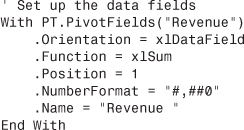
Adding Fields to the Data Area

When you are adding fields to the Data area of the pivot table, there are many settings that you would rather control rather than let Excel’s intellisense decide.

Say that you are building a report with revenue. You likely want to sum the revenue. If you do not explicitly specify the calculation, Excel scans through the data in the underlying data. If 100 percent of the revenue columns are numeric, Excel sums. If one cell is blank or contains text, Excel decides to count the revenue. This produces confusing results.

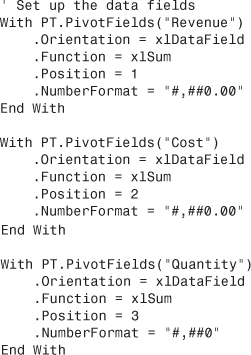
Because of this possible variability, you should never use the DataFields argument in the AddFields method. Instead, change the property of the field to xlDataField. You can then specify the Function to be xlSum.

While you are setting up the data field, you can change several other properties within the same With...End With block.

The Position property is useful when adding multiple fields to the data area. Specify 1 for the first field, 2 for the second field, and so on.

By default, Excel renames a Revenue field to have a strange name like Sum of Revenue. You can use the .Name property to change that heading back to something normal. Note that you cannot reuse the word Revenue as a name, but you can use “Revenue” (with a space).

You are not required to specify a number format, but it can make the resulting pivot table easier to understand and only takes an extra line of code:

Formatting the Pivot Table

Microsoft introduced the Compact Layout for pivot tables in Excel 2007. This means that there are three layouts available in Excel 2010. Excel should default to using the Tabular layout. This is good because tabular view is the one that makes the most sense. It cannot hurt to add one line of code to ensure that you get the desired layout:

PT.RowAxisLayout xlTabularRow

In tabular layout, each field in the row area is in a different column. Subtotals always appear at the bottom of each group. This is the layout that has been around the longest and is most conducive to reusing the pivot table report for further analysis.

The Excel user interface frequently defaults to Compact layout. In this layout, multiple columns fields are stacked up into a single column on the left side of the pivot table. To create this layout, use the following code:

PT.RowAxisLayout xlCompactRow

The one limitation of tabular layout is that you cannot show the totals at the top of each group. If you would need to do this, you want to switch to the Outline layout and show totals at the top of the group:

PT.RowAxisLayout xlOutlineRow
PT.SubtotalLocation xlAtTop

Your pivot table inherits the table style settings selected as the default on whatever computer happens to run the code. If you would like control over the final format, you can explicitly choose a table style. The following code applies banded rows and a medium table style:

At this point, you have given VBA all the settings required to correctly generate the pivot table. If you set ManualUpdate to False, Excel calculates and draws the pivot table. Thereafter, you can immediately set this back to True by using this code:

At this point, you have a complete pivot table like the one shown in Figure 12.4.

Figure 12.4 Fewer than 50 lines of code create this pivot table in less than a second.

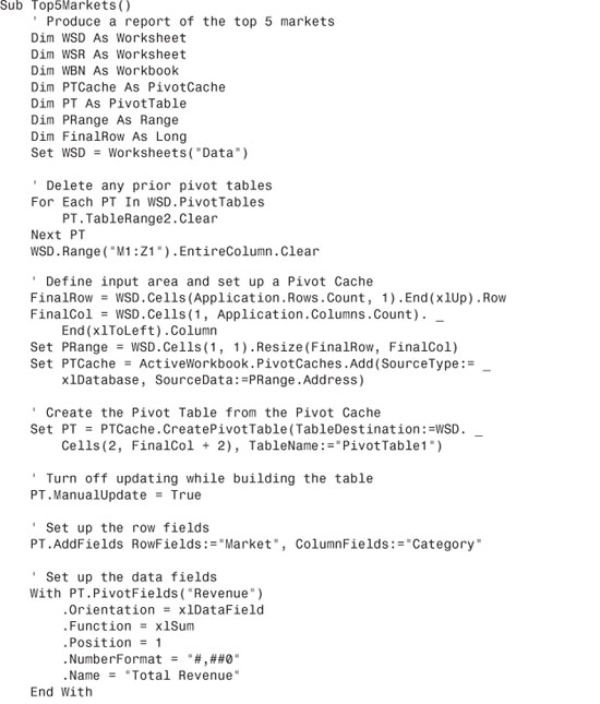
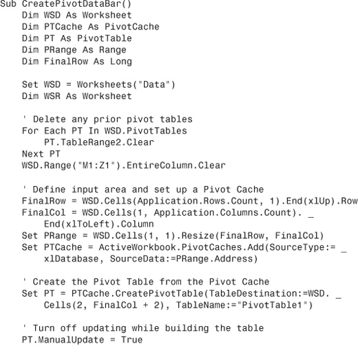
Listing 12.1 shows the complete code used to generate the pivot table.

Listing 12.1 Code to Generate a Pivot Table

Dealing with Limitations of Pivot Tables

As with pivot tables in the user interface, Microsoft maintains tight control over a live pivot table. You need to be aware of these issues as your code is running on a sheet with a live pivot table.

Filling Blank Cells in the Data Area

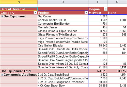
It is always a bit annoying that Excel puts blank cells in the data area of a pivot table. In Figure 12.4, the North region had no sales of a Bar Cover, so that cell appears blank instead of with a zero.

You can override this in the Excel interface by using the For Empty Cells Show setting in the PivotTable Options dialog. The equivalent code is shown here:

PT.NullString = "0"

Filling Blank Cells in the Row Area

Excel 2010 added a much needed setting to fill in the blank cells along the left columns of a pivot table. This problem happens any time that you have two or more fields in the row area of a pivot table. Rather than repeating a label such as “Bar Equipment” in Cells N5:N18, Microsoft traditionally left those cells blank.

To solve that problem in Excel 2010, use:

PT.RepeatAllLabels xlRepeatLabels

Learning Why You Cannot Move or Change Part of a Pivot Report

You cannot use many Excel commands inside of a pivot table. Inserting rows, deleting rows, and cutting and pasting parts of a pivot table are all against the rules.

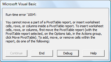
Say that you tried to delete the Grand Total column from Column W in a pivot table. If you try to delete or clear Column W, the macro comes to a screeching halt with an error 1004, as shown in Figure 12.5.

Figure 12.5 You cannot delete just part of a pivot table.

There are two strategies to get around this limitation. The first strategy is to find if there is already an equivalent command in the pivot table interface. For example, there is code to do any of these items:

• Remove the grand total column

• Remove the grand total row

• Add blank rows between each section

• Suppress subtotals for outer row fields

The second strategy is to convert the pivot table to values. You can then insert, cut, and clear as necessary.

Both strategies are discussed in the following sections.

Controlling Totals

The default pivot table includes a grand total row and a grand total column. You can choose to hide one or both of these elements.

To remove the grand total column from the right side of the pivot table, use:

PT.ColumnGrand = False

To remove the grand total row from the bottom of the pivot table, use:

PT.RowGrand = False

Turning off the subtotals rows is surprisingly complex. This issue comes up when you have multiple fields in the row area. Excel automatically turns on subtotals for the outermost row fields.

To suppress the subtotals for a field, you must set the Subtotals property equal to an array of 12 False values. The first False turns off automatic subtotals, the second False turns off the Sum subtotal, the third False turns off the Count subtotal, and so on. This line of code suppresses the Category subtotal:

A different technique is to turn on the first subtotal. This method automatically turns off the other 11 subtotals. You can then turn off the first subtotal to make sure that all subtotals are suppressed:

PT.PivotFields("Category").Subtotals(1) = True
PT.PivotFields("Category").Subtotals(1) = False

Determining Size of a Finished Pivot Table to Convert the Pivot Table to Values

If you plan on converting a live pivot table to values, you need to copy the entire pivot table. This might be tough to predict. If you summarize transactional data every day, you might find that on any given day you do not have sales from one region. This can cause your table to be perhaps seven columns wide on some days and only six columns wide on other days.

Excel provides two range properties that you can use to refer to a pivot table. The .TableRange2 property includes all the rows of the pivot table including any page field drop-downs at the top of the pivot table.

The .TableRange1 property starts just below the filter fields. It does often include the unnecessary row with Sum of Revenue at the top of the pivot table.

If your goal is to convert the pivot table to values and not move the pivot table to a new place, you can use this code:

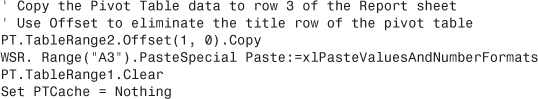
PT.TableRange2.Copy
PT.TableRange2.PasteSpecial xlPasteValues

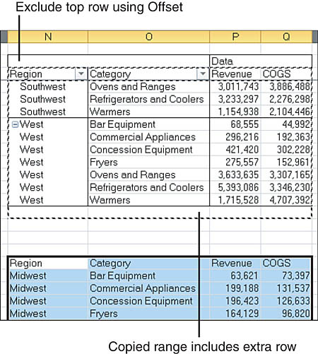
If you want to copy only the data section of the pivot table to a new location, you frequently use the .Offset property to start one row lower than the top of .TableRange2:

PT.TableRange2.Offset(1,0).Copy

This reference copies the data area plus one row of headings.

Notice in the figure that using .OFFSET without .RESIZE causes one extra row to be copied. However, because that row is always blank, there is no need to use .RESIZE to not copy the extra blank row.

The code copies PT.TableRange2 and uses PasteSpecial on a cell six rows below the current pivot table. At that point in the code, your worksheet appears as shown in Figure 12.7. The table in Cell N2 is a live pivot table, and the table in Cell N58 contains the copied results.

Figure 12.7 An intermediate result of the macro. The data at the bottom has been converted to values.

You can then eliminate the pivot table by applying the Clear method to the entire table. If your code is then going on to do additional formatting, you should remove the pivot cache from memory by setting PTCache equal to Nothing.

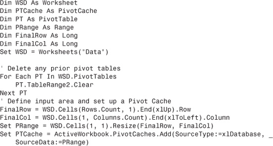
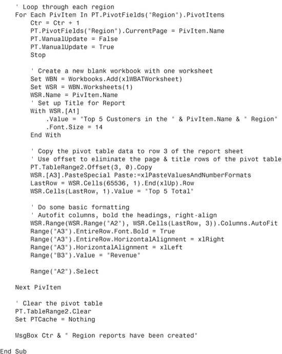
Listing 12.2 uses a pivot table to produce a summary from the underlying data. More than 80,000 rows are reduced to a tight 50 row summary. The resulting data is properly formatted for additional filtering, sorting, and so on. At the end of the code, the pivot table is copied to static values, and the pivot table is cleared.

Listing 12.2 Code to Produce a Static Summary from a Pivot Table

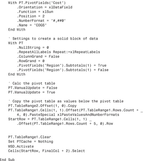
The preceding code creates the pivot table. It then copies the results as values and pastes them below the original pivot table. In reality, you probably want to copy this report to another worksheet or another workbook. Examples later in this chapter introduce the code necessary for this.

So far, this chapter has walked you through building the simplest of pivot table reports. Pivot tables offer far more flexibility. Read on for more complex reporting examples.

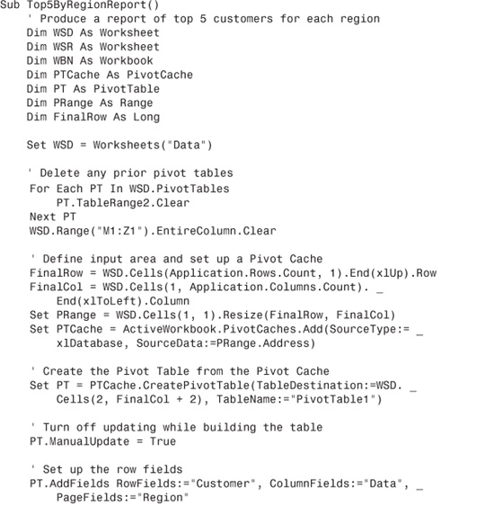
Pivot Table 201: Creating a Report Showing Revenue by Category

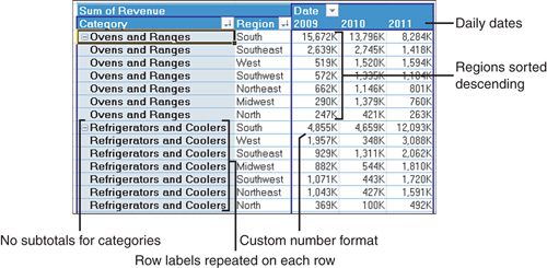
A typical report might provide a list of markets by category with revenue by year. This report could be given to product line managers to show them which markets are selling well. The report in Figure 12.8 is not a pivot table, but the macro to create the report used a pivot table to summarize the data. Regular Excel commands such as Subtotal then finish off the report.

Figure 12.8 This report started as a pivot table, but finished as a regular data set.

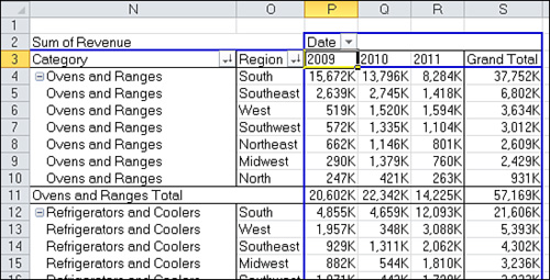
In this example, you want to show the markets in descending order by revenue with years going across the columns. A sample pivot table report is shown in Figure 12.9.

Figure 12.9 A typical request is to take transactional data and produce a summary by product for product line managers.

There are some tricky issues required to create this pivot table:

• You have to roll the daily dates in the original data set up to years.

• You want to control the sort order of the row fields.

• You want to fill in blanks throughout the pivot table, use a better number format, and suppress the subtotals for the category field.

The key to producing this data quickly is to use a pivot table. The default pivot table has a number of quirky problems which you can correct in the macro.

To start, use VBA to build a pivot table with Category and Region as the row fields. Add Date as a column field. Add Revenue as a data field using this code:

Figure 12.10 shows the default pivot table created with these settings.

Figure 12.10 By default, the initial report has many problems.

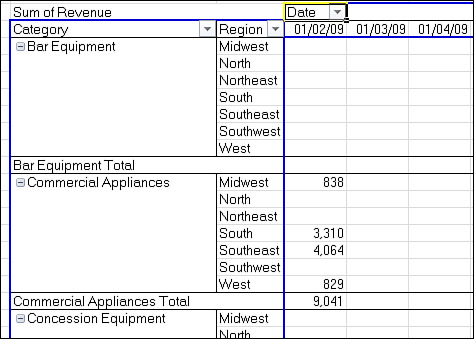
Here are just a few of the annoyances that most pivot tables present in their default state:

• The Outline view is horrible. In Figure 12.10, the value Bar Equipment appears in the product column only once and is followed by six blank cells. Thankfully, Excel 2010 now offers the RepeatAllLabels method to correct this problem. If you intend to repurpose the data, you need the row labels to be repeated on every row.

• Because the original data set contains daily dates, the default pivot table has over a thousand columns of daily data. No one is able to process this report. You need to roll those daily dates up to years. Pivot tables make this easy.

• The report contains blank cells instead of zeros. In Figure 12.10, the entire visible range of Bar Equipment is blank. These cells should contain zeroes instead of blanks.

• The title is boring. Most people would agree that Sum of Revenue is an annoying title.

• Some captions are extraneous. Date floating in the first row of Figure 12.10 does not belong in a report.

• The default alphabetical sort order is rarely useful. Product line managers are going to want the top markets at the top of the list. It would be helpful to have the report sorted in descending order by revenue.

• The borders are ugly. Excel draws in a myriad of borders that make the report look awful.

• Pivot tables offer no intelligent page break logic. If you want to produce one report for each Category manager, there is no fast method for indicating that each product should be on a new page.

• Because of the page break problem, you might find it is easier to do away with the pivot table’s subtotal rows and have the Subtotal method add subtotal rows with page breaks. You need a way to turn off the pivot table subtotal rows offered for Category in Figure 12.10. These rows show up automatically whenever you have two or more row fields. If you had four row fields, you would want to turn off the automatic subtotals for the three outermost row fields.

Even with all these problems in default pivot tables, they are still the way to go. You can overcome each complaint either by using special settings within the pivot table or by entering a few lines of code after the pivot table is created and then copied to a regular data set.

Ensuring Tabular Layout Is Utilized

In legacy versions of Excel, multiple row fields appeared in multiple columns. Three layouts are now available. The Compact layout squeezes all the row fields into a single column.

To prevent this outcome and ensure that your pivot table is in the classic table layout, use this code:

PT.RowAxisLayout xlTabularRow

Rolling Daily Dates Up to Years

With transactional data, you often find your date-based summaries having one row per day. Although daily data might be useful to a plant manager, many people in the company want to see totals by month or quarter and year.

The great news is that Excel handles the summarization of dates in a pivot table with ease. For anyone who has ever had to use the arcane formula =A2+1-Day(A2) to change daily dates into monthly dates, you will appreciate the ease with which you can group transactional data into months or quarters.

Creating a date group with VBA is a bit quirky. The .Group method can be applied to only a single cell in the pivot table, and that cell must contain a date or the Date field label.

In Figure 12.10, you would have to select either the Date heading in Cell P2 or one of the dates in Cells P3:APM3. Selecting one of these specific cells is risky, particularly if the pivot table later starts being created in a new column. Two other options are more reliable.

If you will never use a different number of row fields, then you can assume that the Date heading is in Row 1, Column 3 of the area known as TableRange2. The following line of code would select this cell:

PT.TableRange2.Cells(1, 3).Select

You should probably add a comment that you need to edit the 3 in that line to another number any time that you change the number of row fields.

Another solution is to use the LabelRange property for the Date field. The following code always selects the cell containing the Date heading:

PT.PivotFields("Date").LabelRange.Select

To group the daily dates up to yearly dates, you should define a pivot table with Date in the row field. Turn off ManualCalculation to enable the pivot table to be drawn. You can then use the LabelRange property to locate the date label.

Use the .Group method on the date label cell. You specify an array of seven Boolean values for the Periods argument. The seven values correspond to seconds, minutes, hours, days, months, quarters, and years. For example, to group by years, you would use:

After grouping by years, the field is still called Date. This differs from the results when you group by multiple fields.

To group by months, quarters, and years, you would use:

After grouping up to months, quarters, and years, the Date field starts referring to months. Two new virtual fields are available in the pivot table: Quarters and Years.

To group by weeks, you choose only the Day period, and then use the By argument to group into seven-day periods:

In Figure 12.10, the goal is to group the daily dates up to years, so the following code is used:

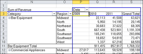
Figure 12.11 shows the pivot table after grouping daily dates up to years.

Figure 12.11 Daily dates have been rolled up to years using the Group method.

Eliminating Blank Cells

The blank cells in a pivot table are annoying. There are two kinds of blank cells that you will want to fix. Blank cells occur in the Values area when there were no records for a particular combination. For example, in Figure 12.11, the company did not sell bar equipment in 2009, so Cells P4:P11 are blank.

Most people would prefer to have zeroes instead of those blank cells. Blank cells also occur in the row labels area when you have multiple row fields. The words Bar Equipment appear in Cell N4, but then Cells N5:N10 are blank. Microsoft added a new property to fill these blank cells in Excel 2010.

To replace blanks in the values area with zeroes, use:

PT.NullString = "0"

To fill in the blanks in the label area in Excel 2010, use:

PT.RepeatAllLabels xlRepeatLabels

The .RepeatAllLabels code fails in Excel 2007 and earlier. The only solution in legacy versions of Excel is to convert the pivot table to values, then set the blank cells to a formula that grabs the value from the row above:

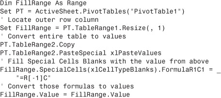
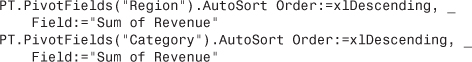
Controlling the Sort Order with AutoSort

The Excel user interface offers a Sort option that enables you to sort a field in descending order based on revenue. The equivalent code in VBA to sort the region and category fields by descending revenue uses the AutoSort method:

Changing Default Number Format

Numbers in the values area of a pivot table need to have a suitable number format applied. You cannot count on the numeric format of the underlying field to carry over to the pivot table.

To show the Revenue values with zero decimal places and a comma, use:

PT.PivotFields("Sum of Revenue").NumberFormat = "#,##0"

Some companies have customers who typically buy thousands or millions of dollars’ worth of goods. You can display numbers in thousands by using a single comma after the number format. To do this, you need to include a K abbreviation to indicate that the numbers are in thousands:

PT.PivotFields("Sum of Revenue").NumberFormat = "#,##0,K"

Local custom dictates the thousands abbreviation. If you are working for a relatively young computer company where everyone uses K for the thousands separator, you are in luck because Microsoft makes it easy to use this abbreviation. However, if you work at a more than 100 year-old soap company where you use M for thousands and MM for millions, you have a few more hurdles to jump. You are required to prefix the M character with a backslash to have it work:

PT.PivotFields("Sum of Revenue").NumberFormat = "#,##0,M"

Alternatively, you can surround the M character with double quotation marks. To put double quotation marks inside a quoted string in VBA, you must put two sequential quotation marks. To set up a format in tenths of millions that uses the #,##0.0,,”MM” format, you would use this line of code:

PT.PivotFields("Sum of Revenue").NumberFormat = "#,##0.0,, ""MM"""

Here, the format is quotation mark, pound, comma, pound, pound, zero, period, zero, comma, comma, space, quotation mark, quotation mark, M,M, quotation mark, quotation mark, quotation mark. The three quotation marks at the end are correct. You use two quotation marks to simulate typing one quotation mark in the custom number format box and a final quotation mark to close the string in VBA.

Figure 12.12 shows the pivot table blanks filled in, numbers shown in thousands, and category and region sorted descending.

Figure 12.12 After filling in blanks and sorting, you only have a few extraneous totals and labels to remove.

Suppressing Subtotals for Multiple Row Fields

As soon as you have more than one row field, Excel automatically adds subtotals for all but the innermost row field. That extra row field can get in the way if you plan on reusing the results of the pivot table as a new data set for some other purpose. In the current example, you have taken 87,000 rows of data and produced a tight 50-row summary of yearly sales by category and region. That new data set would be interesting for sorting, filtering, and charting, if you could remove the total row and the category subtotals. Although accomplishing this task manually might be relatively simple, the VBA code to suppress subtotals is surprisingly complex.

Most people do not realize that it is possible to show multiple types of subtotals. For example, you can choose to show Sum, Average, Min, and Max, as shown in Figure 12.13.

Figure 12.13 Rarely used, the Custom Subtotals option enables many subtotals to be defined for one field.

To suppress subtotals for a field, you must set the Subtotals property equal to an array of 12 False values. The first False turns off automatic subtotals, the second False turns off the Sum subtotal, the third False turns off the Count subtotal, and so on. This line of code suppresses the Category subtotal:

A different technique is to turn on the first subtotal. This method automatically turns off the other 11 subtotals. You can then turn off the first subtotal to make sure that all subtotals are suppressed:

PT.PivotFields("Category").Subtotals(1) = True
PT.PivotFields("Category").Subtotals(1) = False

To remove the grand total row, use

PT.ColumnGrand = False

Copying Finished Pivot Table as Values to a New Workbook

If you plan on repurposing the results of the pivot table, you need to convert the table to values. This section shows you how to copy the pivot table to a brand new workbook.

To make the code more portable, assign object variables to the original workbook, new workbook, and first worksheet in the new workbook. At the top of the procedure, add these statements:

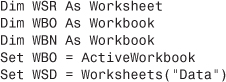
After the pivot table has been successfully created, build a blank Report workbook with this code:

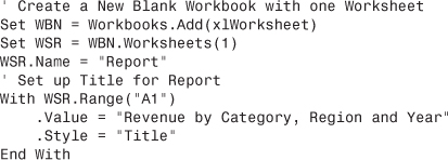
There are a few remaining annoyances in the pivot table. The borders are annoying. There are stray labels such as Sum of Revenue and Date in the first row of the pivot table. You can solve all three of these problems by excluding the first row(s) of PT.TableRange2 from the .Copy method and then using PasteSpecial(xlPasteValuesAndNumberFormats) to copy the data to the report sheet.

In the current example, the .TableRange2 property includes only one row to eliminate, Row 2, as shown in Figure 12.13. If you had a more complex pivot table with several column fields and/or one or more page fields, you would have to eliminate more than just the first row of the report. It helps to run your macro to this point, look at the result, and figure out how many rows you need to delete. You can effectively not copy these rows to the report by using the Offset property. Copy the TableRange2 property, offset by one row.

Purists will note that this code copies one extra blank row from below the pivot table, but this really does not matter because the row is blank. After copying, you can erase the original pivot table and destroy the pivot cache:

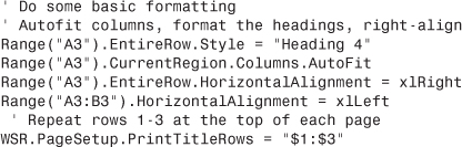
Handling Final Formatting

The last steps for the report involve some basic formatting tasks and then adding the subtotals. You can bold and right-justify the headings in Row 3. Set up rows 1–3 so that the top three rows print on each page:

Adding Subtotals to Get Page Breaks

Automatic subtotals are a powerful feature found on the Data tab. Figure 12.14 shows the Subtotal dialog box. Note the option Page Break Between Groups.

Figure 12.14 Use automatic subtotals because doing so enables you to add a page break after each category. Using this feature ensures that each category manager has a clean report with only her data on it.

If you were sure that you would always have three years and a total, the code to add subtotals for each Line of Business group would be the following:

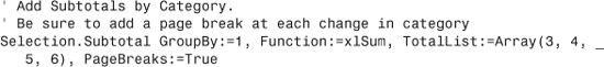
However, this code fails if you have more or less than three years. The solution is to use the following convoluted code to dynamically build a list of the columns to total, based on the number of columns in the report:

Finally, with the new totals added to the report, you need to autofit the numeric columns again with this code:

Putting It All Together

Listing 12.3 produces the product line manager reports in a few seconds.

Listing 12.3 Code That Produces the Category Report in Figure 12.15

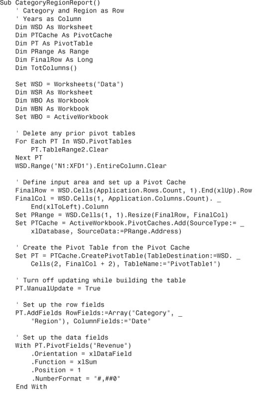
Figure 12.15 Converting 80,000 rows of transactional data to this useful report takes less than two seconds if you use the code that produced this example. Without pivot tables, the code would be far more complex.

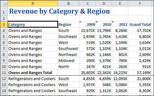
Figure 12.15 shows the report produced by this code.

You have now seen the VBA code to produce useful summary reports from transactional data. The next section will deal with additional features in pivot tables.

Calculating with a Pivot Table

So far, the pivot tables have presented a single field in the values area of the pivot table and that field was always shown as a sum calculation. You can add more fields to the values area. You can change from Sum to any of eleven functions or alter the sum to display running totals, percentage of total, and more. You can also add new calculated fields or calculated items to the pivot table.

Addressing Issues with Two or More Data Fields

It is possible to have multiple fields in the Values section of a pivot report. For example, you might have Quantity, Revenue, and Cost in the same pivot table.

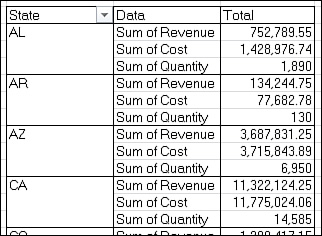
When you have two or more data fields in an Excel 2010 pivot table that you built in the Excel interface, the value fields will go across the columns. However, VBA will build the pivot table with the values fields going down the innermost row field. This creates the bizarre-looking table shown in Figure 12.16.

Figure 12.16 This ugly view was banished in the Excel interface after Excel 2003. VBA still produces it by default.

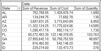
To correct this problem, you should specify that a virtual field called “Data” is one of the column fields.

To have multiple values fields go across the report, use this code:

PT.AddFields RowFields:="State", ColumnFields:="Data"

After adding a column field called Data, you would then go on to define multiple data fields:

This code will produce a pivot table, as shown in Figure 12.17.

Figure 12.17 By specifying the virtual field “Data” as a column field, multiple values go across the report.

Using Calculations Other Than Sum

So far, all of the pivot tables in this chapter have used the Sum function to calculate. There are eleven functions available including Sum. To specify a different calculation, specify one of these values as the .Function property:

• xlAverage—Average.

• xlCount—Count.

• xlCountNums—Count numerical values only.

• xlMax—Maximum.

• xlMin—Minimum.

• xlProduct—Multiply.

• xlStDev—Standard deviation, based on a sample.

• xlStDevP—Standard deviation, based on the whole population.

• xlSum—Sum.

• xlVar—Variation, based on a sample.

• xlVarP—Variation, based on the whole population.

Note that when you add a field to the Values area of the pivot table, Excel modifies the field name with the function name and the word “of”. For example, “Revenue” becomes “Sum of Revenue”. “Cost” might become “StdDev of Cost”. If you later need to refer to those fields in your code, you need to refer to them using the new name such as “Average of Quantity”.

You can improve the look of your pivot table by changing the .Name of the field. If you do not want the words “Sum of Revenue” appearing in the pivot table, change the .Caption to “Total Revenue”. This sounds less awkward than “Sum of Revenue”. Remember that you cannot have a name that exactly matches an existing field name in the pivot table. “Revenue” is not suitable as a name. “Revenue” (with a leading space) is fine to use as a name.

For text fields, the only function that makes sense is a count. You will frequently count the number of records by adding a text field to the pivot table and using the count function.

The following code fragment will calculate total revenue, a count of records by counting a text field, and average quantity:

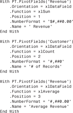
Figure 12.18 shows the pivot table that would result from this code.

Figure 12.18 You can change the function used to summarize columns in the value area of the pivot table.

Generating a Count Distinct

Note that the Count function is not a Count Distinct. If you have seven line items per invoice and ask for a Count of Invoice Number, the function will return the total number of line items, not the number of unique invoice numbers.

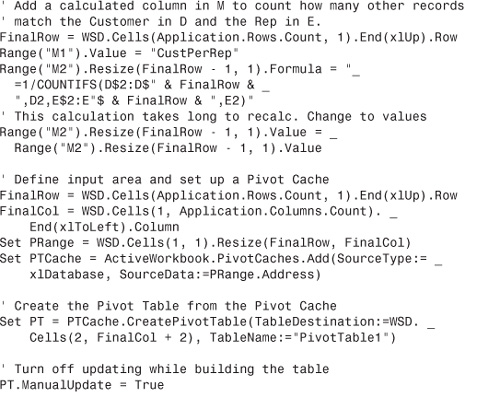
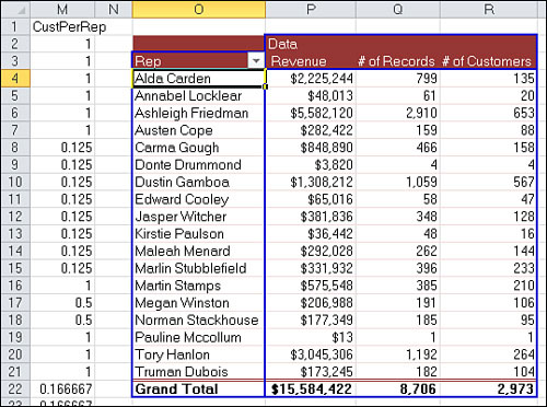
There is a clever workaround to find the count distinct. Say that you want to figure out how many unique customers were handled by each sales rep. Add a new formula to the original data set that will figure out how many other records in the data set match both the customer name and sales rep name for the current row’s records. Once you know this number, divide it into the number 1. You will then sum this field in the pivot table to produce a count of the distinct number of customers per sales rep.

If this sounds confusing, it is. Follow this logic: say that a particular customer placed 17 orders with their sales rep this year. The COUNTIFS portion of this formula will calculate that a total of 17 records have this customer name and sales rep name. When you divide 1/17, you will get 0.058824 for each of those records. When the pivot table sums that field, those 17 records will appear as a 1 in the result!

The formula to code below will add this formula as a new Column M of the original data set:

1/COUNTIFS($D$2:$D$87061,D2, $E$2:$E$87061,E2)

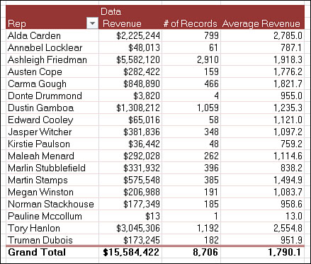
The following code fragment will produce a pivot table that contrasts the count of customer with the sum of this calculated field:

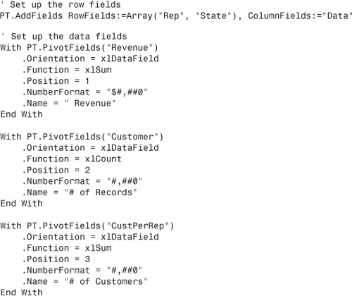
The results of the pivot table are shown in Figure 12.19. Although Column R is a “count of customer,” it really shows the total number of records for the customers. The results in Column S make use of the CustPerRep field and show a true Count Distinct calculation.

Figure 12.19 Calculating a distinct number of customers requires a new formula in the original data set.

Calculated Data Fields

Pivot tables offer two types of formulas. The most useful type defines a formula for a calculated field. This adds a new field to the pivot table. Calculations for calculated fields are always done at the summary level. If you define a calculated field for average price as Revenue divided by Units Sold, Excel first adds the total revenue and total quantity, and then it does the division of these totals to get the result. In many cases, this is exactly what you need. If your calculation does not follow the associative law of mathematics, it might not work as you expect.

To set up a calculated field, use the Add method with the CalculatedFields object. You have to specify a field name and a formula.

PT.CalculatedFields.Add "ACS", Formula:="=Revenue /CustPerRep"

Once you define the field, add it as a data field:

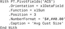
Note that the field is calculating an average, but the function is a sum. This forces Excel to use a label such as “Sum of ACS”. Use the .Caption property to insert a different label in the actual pivot table.

Figure 12.20 shows a report with the calculated field.

Figure 12.20 A calculation in the original data set and a calculated field in the pivot table produce average customer size per sales rep.

Calculated Items

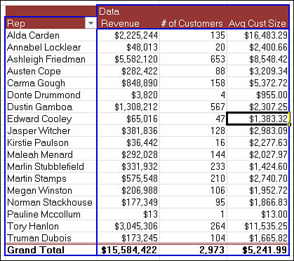
Calculated items have the potential to produce incorrect results in your pivot table. Say that you have a report of sales by eight states. You want to show a subtotal of four of the states. A calculated item would add a ninth item to the state column. While the pivot table would gladly calculate this new item, it will cause the grand total to appear overstated.

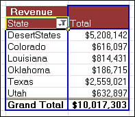
Figure 12.21 shows a pivot table with these eight states. The total revenue is $10 million. When a calculated item provides a subtotal of four states (see Figure 12.22), the grand total increases to $15 million. This means that the items that make up the calculated item are included in the total twice. If you like restating numbers to the Securities and Exchange Commission, feel free to use calculated items.

Figure 12.21 This pivot table adds up to $10 Million.

Figure 12.22 Add a calculated item and the total is overstated.

The code to produce the calculated item is shown here. Calculated items are added as the final position along the field, so this code changes the .Position property to move the Desert States item to the proper position:

If you hope to use a calculated item, you should either remove the grand total row or remove the four states that go into the calculated item. This code hides the four states. The resulting pivot table returns to the correct total, as shown in Figure 12.23:

Figure 12.23 One way to use calculated items is to remove any elements that went into the calculated item.

A better solution, which is discussed in the next section, is to skip Calculated Items and to use text grouping.

Calculating Groups

If you need to calculate subtotals for certain regions, a better solution is to use text grouping to define the groups. If you group the four states, Excel will add a new field to the row area of the pivot table.

Although this process requires some special handling, it is worthwhile and creates a nice-looking report.

To group four states in the Excel interface, you would select the cells that contain those four states and select Group Selection from the PivotTable Tools Options tab. This immediately does several things:

• The items in the group are moved together in the row area.

• A new field is added to the left of the state field. If the original field was called “State”, the new field will be called “State2”.

• Annoyingly, the subtotals property for the new State2 field is set to None instead of Automatic.

• A subtotal for the selected items is added with the name of “Group1”.

• Any items not in a group have a new subtotal added to State2 with the state name repeated.

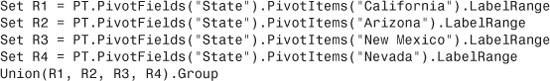
In VBA, it is somewhat tricky to select the cells that contain the proper states. The following code uses the LabelRange property to point to the cells and then uses the UNION method to refer to the four non-contiguous cells:

After setting up the first group, rename the newly created States2 field to have a suitable name:

PT.PivotFields("State2").Caption = "State Group"

Then, change the name of this region from Group1 to the desired group name:

PT.PivotFields("State Group").PivotItems("Group1").Caption = "Desert States"

Change the subtotals property to Automatic from None:

PT.PivotFields("State Group").Subtotals(1) = True

Once you have set up the first group, you can define the remaining groups with this code:

The result is a pivot table with new virtual groups as shown in Figure 12.24.

Figure 12.24 Grouping text fields allows for reporting by territories that are not in the original data.

Using Show Values As to Perform Other Calculations

The Show Values As drop-down on the Options tab offers 15 different calculations available. These calculations allow you to change from numbers to percentage of total, running totals, ranks, and more.

Change the calculation by using the .Calculation option for the pivot field.

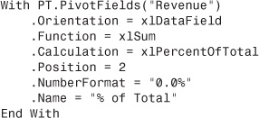
Some calculations such as % of Column or % of Row need no further definition; you do not have to specify a base field. Here is code to show revenue as a percentage of total revenue:

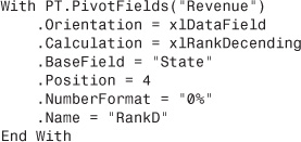
Other calculations need a base field. If you are showing revenue and ask for the descending rank, you could specify that the base field is the state field. In this case, you are asking for this state’s rank based on revenue:

A few calculations require both a base field and a base item. If you wanted to show every state’s revenue as a percentage of California revenue, you would have to specify % Of as the calculation, state as the base field and California as the base item:

Some of the calculations fields are new in Excel 2010. In Figure 12.25, Column I uses the new % of Parent calculation and Column H uses the old % of Total calculation. In both columns, Desert States is 52% of the Grand Total (Cells H8 and I8). However, Cell I5 shows that California is 60.8% of Desert States, while Cell H5 shows that California is 31.6% of the grand total.

Figure 12.25 % of Parent in Column I is new in Excel 2010.

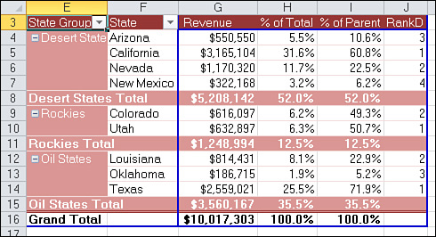
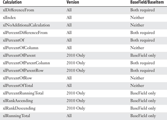
Table 12.4 shows the complete list of .Calculation options. The second column indicates if the calculation is compatible with previous versions of Excel. The third column indicates if you need a base field and base item.

Table 12.4 Calculation Options Available in Excel 2010 VBA

Using Advanced Pivot Table Techniques

Even if you are a pivot table pro, you may never have run into some of the really advanced techniques available with pivot tables. The following sections discuss such techniques.

Using AutoShow to Produce Executive Overviews

If you are designing an executive dashboard utility, you might want to spotlight the top five markets.

This setting lets you select either the top or bottom n records based on any data field in the report.

The code to use AutoShow in VBA uses the .AutoShow method:

When you create a report using the .AutoShow method, it is often helpful to copy the data and then go back to the original pivot report to get the totals for all markets. In the following code, this is achieved by removing the Market field from the pivot table and copying the grand total to the report. Listing 12.4 produces the report shown in Figure 12.26.

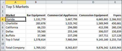
Figure 12.26 The Top 5 Markets report contains two pivot tables.

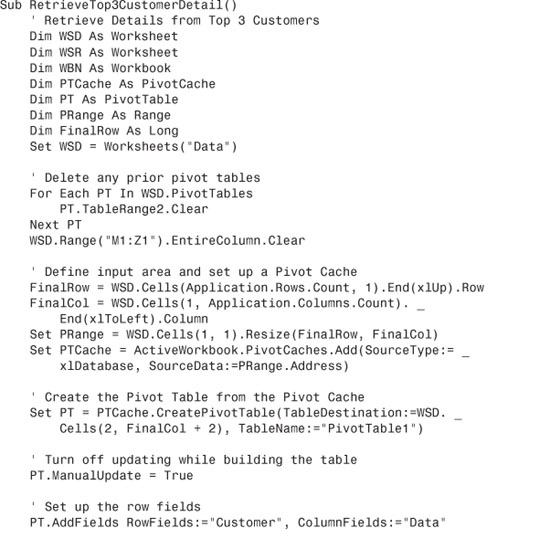
Listing 12.4 Code Used to Create the Top 5 Markets Report

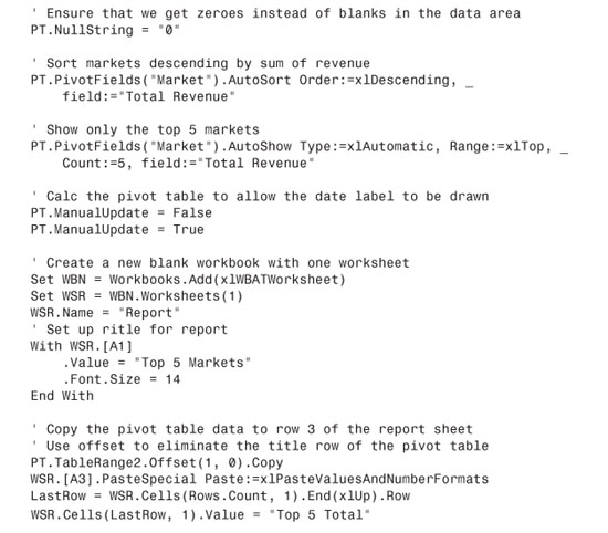
The Top 5 Markets report actually contains two snapshots of a pivot table. After using the AutoShow feature to grab the top five markets with their totals, the macro went back to the pivot table, removed the AutoShow option, and grabbed the total of all markets to produce the Total Company row.

Using ShowDetail to Filter a Recordset

Take any pivot table in the Excel user interface. Double-click any number in the table. Excel inserts a new sheet in the workbook and copies all the source records that represent that number. In the Excel user interface, this is a great way to perform a drill-down query into a data set.

The equivalent VBA property is ShowDetail. By setting this property to True for any cell in the pivot table, you generate a new worksheet with all the records that make up that cell:

PT.TableRange1.Offset(2, 1).Resize(1, 1).ShowDetail = True

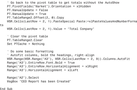
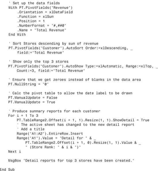
Listing 12.5 produces a pivot table with the total revenue for the top three stores and ShowDetail for each of those stores. This is an alternative method to using the Advanced Filter report. The results of this macro are three new sheets. Figure 12.27 shows the first sheet created.

Figure 12.27 Pivot table applications are incredibly diverse. This macro created a pivot table of the top three stores and then used the ShowDetail property to retrieve the records for each of those stores.

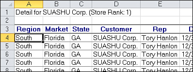
Listing 12.5 Code Used to Create a Report for Each of the Top Three Customers

Creating Reports for Each Region or Model

A pivot table can have one or more Report Filter fields. A Report Filter field goes in a separate set of rows above the pivot report. It can serve to filter the report to a certain region, certain model, or certain combination of region and model. In VBA, Report Filter fields are called page fields.

You might create a pivot table with several filter fields in order to allow someone to do adhoc analyses. However, it is more likely that you will use the filter fields in order to produce reports for each region.

To set up a report filter in VBA, add the PageFields parameter to the AddFields method. The following line of code creates a pivot table with Region in the Report Filter:

PT.AddFields RowFields:= "Product", _
   ColumnFields:= "Data", PageFields:= "Region"

The preceding line of code sets up the Region report filter with the value (All), which returns all regions. To limit the report to just the North region, use the CurrentPage property:

PT.PivotFields("Region").CurrentPage = "North"

One use of a report filter is to build a user form in which someone can select a particular region or particular product. You then use this information to set the CurrentPage property and display the results of the user form.

One amazing trick is to use the Show Pages feature to replicate a pivot table for every item in one filter field drop-down. After creating and formatting a pivot table, you can run this single line of code. If you have eight regions in the data set, eight new worksheets will be inserted in the workbook, one for each region. The pivot table will appear on each worksheet, with the appropriate region chosen from the drop-down:

PT.ShowPages PageField:=Region

To determine how many regions are available in the data, use PT.PivotFields("Region").PivotItems.Count. Either of these loops would work:

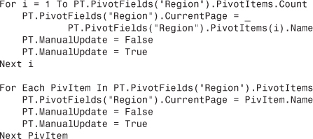
Of course, in both of these loops, the three region reports fly by too quickly to see. In practice, you would want to save each report while it is displayed.

So far in this chapter, you have been using PT.TableRange2 when copying the data from the pivot table. The TableRange2 property includes all rows of the pivot table, including the page fields. There is also a .TableRange1 property, which excludes the page fields. You can use either statement to get the detail rows:

PT.TableRange2.Offset(3, 0)
PT.TableRange1.Offset(1, 0)

Which you use is your preference, but if you use TableRange2, you will not have problems when you try to delete the pivot table with PT.TableRange2.Clear. If you were to accidentally attempt to clear TableRange1 when there are page fields, you would end up with the dreaded "Cannot move or change part of a pivot table" error.

Listing 12.6 produces a new workbook for each region, as shown in Figure 12.28.

Figure 12.28 By looping through all items found in the Region page field, the macro produced one workbook for each regional manager.

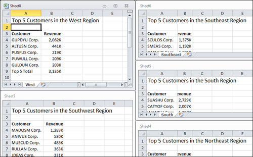
Listing 12.6 Code That Creates a New Workbook Per Region

Manually Filtering Two or More Items in a PivotField

In addition to setting up a calculated pivot item to display the total of a couple of products that make up a dimension, you can manually filter a particular PivotField.

For example, you have one client who sells shoes. In the report showing sales of sandals, he wants to see just the stores that are in warm-weather states. The code to hide a particular store is:

PT.PivotFields("Store").PivotItems("Minneapolis").Visible = False

You need to be very careful never to set all items to False; otherwise, the macro ends with an error. This tends to happen more than you would expect. An application may first show products A and B and then on the next loop show products C and D. If you attempt to make A and B not visible before making C and D visible, no products will be visible along the PivotField, which causes an error. To correct this, always loop through all PivotItems, making sure to turn them back to visible before the second pass through the loop.

This process is easy in VBA. After building the table with Product in the page field, loop through to change the Visible property to show only the total of certain products:

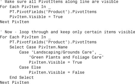
Using the Conceptual Filters

Beginning with Excel 2007, conceptual filters for date fields, numeric fields, and text fields are provided. In the PivotTable Field List, hover the mouse cursor over any active field in the field list portion of the dialog box. In the drop-down that appears, you can choose Label Filters, Date Filters, or Value Filters.

To apply a label filter in VBA, use the PivotFilters.Add method. The following code filters to the Customers that start with 1:

PT.PivotFields("Customer").PivotFilters.Add _
    Type:=xlCaptionBeginsWith, Value1:="1"

To clear the filter from the Customer field, use the ClearAllFilters method:

PT.PivotFields("Customer").ClearAllFilters

To apply a date filter to the date field to find records from this week, use this code:

PT.PivotFields("Date").PivotFilters.Add Type:=xlThisWeek

The value filters allow you to filter one field based on the value of another field. For example, to find all the markets where the total revenue is over $100,000, you would use this code:

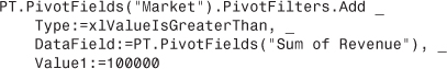
Other value filters might allow you to specify that you want branches where the revenue is between $50,000 and $100,000. In this case, you would specify one limit as Value1 and the second limit as Value2:

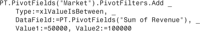
Table 12.5 lists all the possible filter types.

Table 12.5 Filter Types

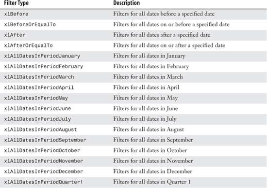
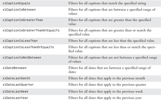
Using the Search Filter

Excel 2010 added a Search box to the filter drop-down. While this is a slick feature in the Excel interface, there is no equivalent magic in VBA. While Figure 12.29 shows the “Select All Search Results” check box, the equivalent VBA simply lists all of the items that match the selection.

Figure 12.29 The Excel 2010 interface offers a search box. In VBA, you can emulate using the old xlCaptionContains filter.

There is nothing new in Excel 2010 VBA to emulate the search box. To achieve the same results in VBA, use the xlCaptionContains filter described in the previous section.

Setting Up Slicers to Filter a Pivot Table

Excel 2010 introduced the concept of slicers to filter a pivot table. A slicer is a visual filter. Slicers can be resized and repositioned. You can control the color of the slicer and control the number of columns in a slicer. You can also select or clear items from a slicer using VBA.

Figure 12.30 shows a pivot table with two slicers. The State slicer has been modified to have five columns. The slicer with a caption of “Territory” is actually based on the Region field. You can give the slicers a friendlier caption which might be helpful when the underlying field is called IDKTxtReg or some other bizarre name invented by the I.T. department.

Figure 12.30 Slicers provide a visual filter for State and Region.

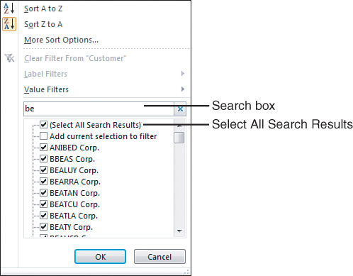
A slicer is comprised of a SlicerCache and a Slicer. To define a slicer cache, you need to specify a pivot table as the source and a field name as the SourceField. The SlicerCache is defined at the workbook level. This allows you to have the Slicer on a different worksheet than the actual pivot table:

Once you have defined the slicer cache, you can add the slicer. The slicer is defined as an object of the slicer cache. Specify a worksheet as the destination. The name argument controls the internal name for the slicer. The Caption argument is the heading that will be visible in the slicer. Specify the size of the slicer using height and width in points. Specify the location using top and left in point. In the code below, the values for top, left, height, and width are assigned to be equal to the location or size of certain cell ranges:

All slicers start out as one column. You can change the style and number of columns with this code:

Once the slicer is defined, you can actually use VBA to choose which items are activated in the slicer. It seems counter-intuitive, but to choose items in the slicer, you have to change the SlicerItem, which is a member of the SlicerCache, not a member of the slicer:

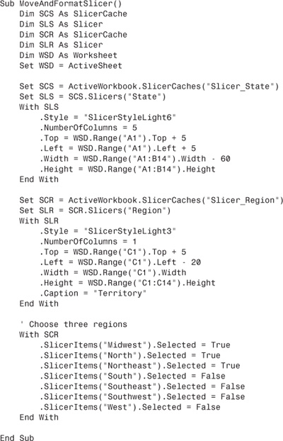
You might need to deal with slicers that already exist. If a slicer is created for the state field, the name of the SlicerCache will be “Slicer_State”. The following code was used to format the slicers in Figure 12.30:

Filtering an OLAP Pivot Table Using Named Sets

Ready for some Good News, Bad News, and Sneaky News?

Good News

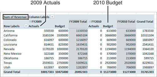
Microsoft added an amazing feature to Excel 2010 pivot tables called Named Sets. This feature allows you to create filters that were never possible before. For example, in Figure 12.31, the pivot table shows Actuals and Budget for FY2009 and FY2010. It would have been impossible to show an asymmetric report with only FY2009 Actuals and FY 2010 Budget: when you turned off Budget for 2009, it would have been turned off for all years. Named Sets allow you to overcome this.

Figure 12.31 You want to show 2009 Actuals and 2010 Budget.

Bad News

Named sets only work for data coming from OLAP pivot tables. If you are dealing with pivot tables based on regular Excel data, you will have to wait until a future release of Excel to tap into the power of Named Sets.

Sneaky News

A pivot table produced using the PowerPivot add-in is actually an OLAP pivot table. To create the pivot table shown in Figure 12.31, you can copy the Excel data, paste as a new table in the PowerPivot Add-in, and then return to Excel to create the pivot table.

This is a minor use for a powerful tool. The PowerPivot add-in is designed to mash-up multi-million row record sets from various sources. To take a single flat table and paste it into the powerful tool is admittedly underutilizing the tool. However, it is one great way to get an unbalanced pivot table report.

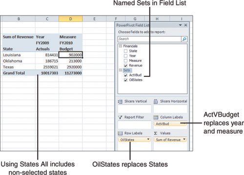
One common use for named sets is to show only a subset of items. For example, you might only be responsible for the states of Louisiana, Oklahoma and Texas. If this grouping is not defined in the data, you will find yourself constantly re-filtering the report to include only your states. Defining a named sets creates a virtual column that contains only your states. This virtual column can be re-used across many reports.

Another common use is to show an asymmetric selection from two column fields. In Figure 12.31, you would like to show last year’s actual and this year’s budget.

To define a named set, you will have to build a formula that uses the MDX language. MDX stands for Multidimensional Expressions Language. There are many MDX tutorials on the Internet. Luckily, you can turn on the macro recorder while you define a named set using the Excel 2010 interface and have the macro recorder write the MDX formula for you.

When you are defining a named set, you will define both a CalculatedMember and then add a CubeField Set. These declarations at the top of the macro initialize two calculated members:

The MDX Formula is the key to the named set. In this code, the formula contains three specific states plus the grand total of all the states. The formula starts and ends with curly braces indicating that the formula contains an array of values. Each line of code is adding another specific state to the array:

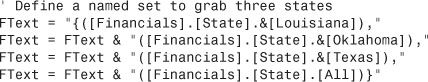
Once you have defined the formula, use the following code to add the calculated member to the data set:

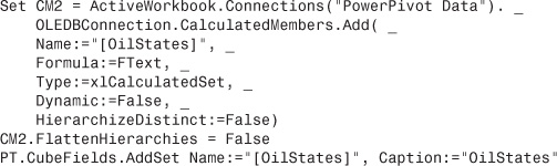
This code will add a new folder to the pivot table field list called Sets. In that folder, an item called OilStates is available as field just like the field called States. In your code, you need to replace the States field in the pivot table with the OilStates field:

Figure 12.32 shows the asymmetric report.

Figure 12.32 Named sets enable asymmetric reporting.

Formatting a Pivot Table

There are a number of options available when formatting a pivot table. This section will cover the layout options, style options from the Design tab, and applying a data visualization to a pivot table.

Applying a Table Style

The Design tab offers two groups dedicated to formatting the pivot table, as shown in Figure 12.33. The PivotTable Style Options group has four check boxes that modify the styles in the PivotTable Styles Gallery.

Figure 12.33 The four check boxes and gallery of styles offer many variations for formatting the pivot table.

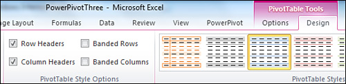
The following four lines of code are equivalent to selecting all four settings in the PivotTable Style Options group:

To apply a table style from the gallery, use the TableStyle2 property. If you want to get the correct name, it might be best to record a macro:

Changing the Layout

The Layout group of the Design tab contains four drop-downs. These drop-downs control the location of subtotals (top or bottom), the presence of grand totals, the report layout, and the presence of blank rows.

Subtotals can appear either at the top or bottom of a group of pivot items. The SubtotalLocation property applies to the entire pivot table; valid values are xlAtBottom or xlAtTop:

PT.SubtotalLocation:=xlAtTop

Grand totals can be turned on or off for rows or columns. The following code turns them off for both:

PT.ColumnGrand = False
PT.RowGrand = False

There are three settings for the report layout. The Tabular layout is similar to the default layout in Excel 2003. The Outline layout was optionally available in Excel 2003. The Compact layout was introduced in Excel 2007.

Excel can remember the last layout used and will apply it to additional pivot tables created in the same Excel session. For this reason, you should always explicitly choose the layout that you want. Use the RowAxisLayout method; valid values are xlTabularRow, xlOutlineRow, or xlCompactRow:

Starting in Excel 2007, you can add a blank line to the layout after each group of pivot items. Although the Design tab offers a single setting to affect the entire pivot table, the setting is actually applied to each individual pivot field individually. The macro recorder responds by recording a dozen lines of code for a pivot table with 12 fields. You can intelligently add a single line of code for the outer row field(s):

PT.PivotFields("Region").LayoutBlankLine = True

Applying a Data Visualization

Excel 2007 introduced fantastic data visualizations such as icon sets, color gradients, and in-cell data bars. When you apply a visualization to a pivot table, you should exclude the total rows from the visualization.

If you have 30 branches that average $50,000 in revenue each, the total for the 30 branches is $1.5 million. If you include the total in the data visualization, the total gets the largest bar, and all the branch records have tiny bars.

Figure 12.34 shows a solution; apply the visualization to the category records but not to the grand total row.

Figure 12.34 Data bars in a pivot table should exclude the Grand Total cell.

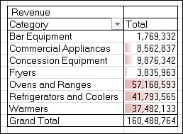
In the Excel user interface, you always want to use the Add Rule or Edit Rule choice to select the option All Cells Showing “Sum of Revenue” for “Category”.

In VBA, you can limit the data bar to only the detail rows by using this code:

Selection.FormatConditions(1).ScopeType = xlFieldsScope

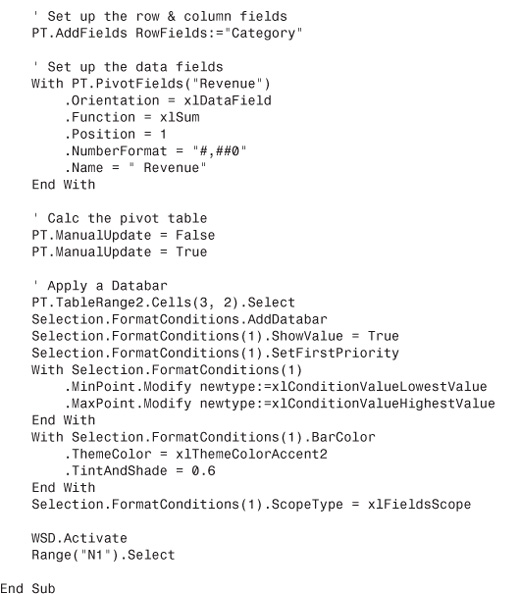
The code in Listing 12.7 adds a pivot table and applies a data bar to the revenue field.

Listing 12.7 Code That Creates a Pivot Table with Data Bars

Next Steps

In the next chapter, you will learn a myriad of techniques for handling common questions and issues with pivot tables.