14. Dr. Jekyll and Mr. GetPivotData

This chapter shows you a technique that solves many annoying pivot table problems. If you have been using pivot tables for a while, you might have run into these problems:

• Formatting tends to be destroyed when you refresh your pivot table. Numeric formats are lost. Column widths go away.

• There is no way to build an asymmetric pivot table. Named Sets offer hope, but only for those using OLAP data or those who have the time to convert their Excel data to the PowerPivot window.

• Excel cannot remember a template. If you frequently have to re-create a pivot table, you must redo the groupings, calculated fields, calculated items, and so on.

The techniques in this chapter solve all those problems. They are not new. In fact, they have been around since Excel 2002.

I have taught Power Excel seminars to thousands of accountants who use Excel 40–60 hours a week. Out of those thousands of people, I have only had three people say that they use this technique.

Ironically, far more than 0.3 percent of people know of this feature. One common question that I get at seminars is, “Why did this feature show up in Excel 2002, and how the heck can you turn it off?”

This same feature, which is reviled by most Excellers, is the key to creating reusable pivot table templates.

The credit for this chapter must go to Rob Collie, who spent years on the Excel project management team. He spent this last development cycle working on the PowerPivot product. Rob happened to relocate to Cleveland, Ohio. Because Cleveland is not a hotbed of Microsoft developers, Dave Gainer gave me a heads-up that Rob was moving to my area, and we started having lunch.

Rob and I talked about Excel and had great conversations. During our second lunch, Rob said something that threw me for a loop. He said, “We find that our internal customers use GetPivotData all the time to build their reports, and we are not sure they will like the way PowerPivot interacts with GetPivotData.”

I stopped Rob to ask if he was crazy. I told him that in my experience with about 5,000 accountants, only three of them had ever admitted to liking GetPivotData. What did he mean that he finds customers actually using GetPivotData?

Rob explained the key word in his statement. He was talking about internal customers, which are the people inside Microsoft who use Excel to do their jobs. Those people had become incredibly reliant on GetPivotData. He agreed that outside of Microsoft, hardly anyone ever uses GetPivotData. In fact, the only question he ever gets outside of Microsoft is how to turn off the stupid feature.

I had to know more, so I asked Rob to explain how the evil GetPivotData could ever be used for good purposes. Rob explained it to me, and I use this chapter to explain it to you.

However, I know that 99 percent of you are reading this chapter because:

• You ran into the evil GetPivotData.

• You turned to the index of this book to find information on GetPivotData.

• You are expecting me to tell you how to turn off GetPivotData.

So, let’s start there.

Turning Off the Evil GetPivotData Problem

GetPivotData has been the cause of so many headaches. All of a sudden, around the time of Excel 2002, without any fanfare, pivot table behavior changed slightly. Any time you build formulas outside of a pivot table that point back inside the pivot table, you run into this evil problem.

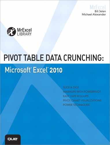
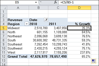
Say you built a pivot table, as shown in Figure 14.1. Those years across the top are built by grouping daily dates up to years. You would like to compare this year versus last year. Unfortunately, you are not allowed to add calculated items to a grouped field.

Figure 14.1 You want to add a formula to show % Growth year after year.

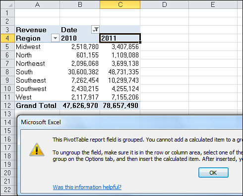
Add a % Growth heading in Cell D4. Copy the formatting from C4 over to D4. In Cell D5, type an equal sign. Click Cell C5. Type a / (slash) for division. Click B5. Type -1 and press Ctrl+Enter to stay in the same cell.

Format the result as a percentage. You see that the Midwest region grew by 35.3 percent. That is impressive growth. It is good to see that the economic woes of late 2009 and 2010 are now gone (see Figure 14.2).

Figure 14.2 Build the formula in D5 using the mouse or the arrow keys.

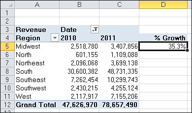
After entering your first formula, select Cell D5. Double-click the tiny square dot in the lower right corner of the cell. This is the Fill Handle, and it copies the formula down to the end of the report.

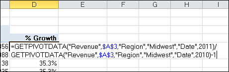
Immediately, you notice something is wrong because every region managed to grow by exactly 35.3 percent (see Figure 14.3).

Figure 14.3 When the formula is copied down, somehow the growth was 35.3 percent for every region.

There is no way that this happens in real life. The data must be fabricated. Look around. Are you working at Enron? If not, then there must be another solution.

Think about the formula you built: 2011 divided by 2010 minus 1. You probably could create that formula with your eyes closed. (Okay, people who used a mouse could not actually do it with their eyes closed, but the people who built the formula using arrow keys probably could without looking at the screen.)

That is what allows you not to notice something completely evil when you built the formula. When you went through the steps to build the formula, any rational person would expect Excel to create a formula such as =C5/B5-1.

However, go back to Cell D5 and press the F2 to look at the formula (see Figure 14.4). Something evil has happened. The simple formula of =C5/B5-1 is no longer there. Instead, Excel generated some GetPivotData nonsense. Although the formula works in D5, it is not working when you copy the formula down.

Figure 14.4 What is GetPivotData?

When this occurs, your reaction is something like, “What is GetPivotData, and why is it screwing up my report?” Your next reaction is, “How can I turn it off?” If it is not a pressure cooker of a day, you might even wonder, “Why would Microsoft put this evil thing in there?”

I am sure this never happened back in Excel 2000. After being stung by GetPivotData repeatedly, I hated GetPivotData. I was thrown for a loop in one of the Power Analyst Boot Camps when someone stopped to ask me how it could possibly be used. I had never considered that question. In my mind, and in most people’s minds, GetPivotData was evil and no good.

Great news—there are two ways to turn it off, which are presented in the next sections.

Preventing GetPivotData by Typing the Formula

The simple method for avoiding GetPivotData is to create your formula without touching the mouse or the arrow keys. To do this, follow these steps:

1. Go to Cell D5; type = (equal sign).

2. Type C5.

3. Type the / (slash sign for division).

4. Type B5.

5. Type -1.

6. Press Enter.

You have now built a regular Excel formula that can be copied down to produce real results, as shown in Figure 14.5.

Figure 14.5 Type =C5/B5-1 and the formula works as expected.

It is a relief to see you can still build formulas outside of pivot tables that point into a pivot tables. I have run into people who simply thought this could not be done.

You might be a bit annoyed that you have to abandon your normal way of entering formulas. If so, the next section offers an alternative.

GetPivotData Is Surely Evil—Turn It Off

If you do not plan to read the second half of this chapter, you can simply turn off GetPivotData forever. Who needs it? It is evil—just turn it off.

Back in Excel 2002 and Excel 2003, it was hard to turn off. You had to go to Tools, Customize, Commands. Select Data from the left listbox, then scroll 83 percent of the way through the right listbox to find an icon called Generate GetPivotData. Drag that icon onto the Excel 2003 toolbar. Close the dialog. Click the icon once to turn it off. Then, you could Alt+Drag the icon off the toolbar because you would never need to turn on this evil feature again.

In Excel 2010, follow these steps:

1. Move the cell pointer back inside a pivot table so that the PivotTable Tools tabs appear.

2. Click the Options tab.

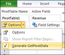
3. Notice the Options icon on the left side of the Ribbon (see Figure 14.6). Do not click the icon. Next to the options icon there is a drop-down arrow. Click the drop-down arrow.

Figure 14.6 Don’t click the large Options icon. Click the tiny dropdown arrow next to the icon.

4. Inside the Options drop-down, there is a choice for Generate GetPivotData (see Figure 14.7). By default, this option is selected. Click that item to clear this check box.

Figure 14.7 Select Generate GetPivotData to turn the feature off.

The previous steps assume that you have a pivot table in the workbook that you can select in order to access the PivotTable tabs. If you don’t have a pivot table in the current workbook, you can use File, Options. In the Formulas category, uncheck Use GetPivotData functions for PivotTable References.

Why Did Microsoft Force GetPivotData on Us?

If GetPivotData is so evil, why did the fine people at Microsoft turn on that feature by default? Everyone simply turns it off. Why would they bother to leave it on? Are they trying to make sure that there is a market for my Power Excel seminars?

I have a theory about this that I came up with during the Excel 2007 launch. I had written many books about Excel 2007, somewhere around 1800 pages of content. When the Office 2007 launch events were happening around the country, I was given an opportunity to work at the event. I watched with interest when the presenter talked about the new features in Excel 2007.

There were at least 15 amazing features in Excel 2007. The presenter took three minutes and glossed over perhaps two and a half of the features.

I was perplexed. How could Microsoft marketing do such a horrible job of showing what was new in Excel?

Then, I realized that this must always happen. Marketing asks the development team what is new. The project manager gives them a list of 15 items. The marketing guy says something like, “There is not room for 15 items in the presentation. Can you cut 80 percent of those items out of the list and give me just the ones with glitz and sizzle?”

Whoever worked on GetPivotData certainly knew that GetPivotData would never have enough sizzle to make it into the marketing news about Excel 2002. So, by making it the default, they hoped someone would notice GetPivotData and try to figure out how it could be used. Instead, most people, including me, just turned it off and thought it was another step in the Microsoft plot to make our lives miserable by making it harder to work in Excel.

Using GetPivotData to Solve Pivot Table Annoyances

You would not be reading this book if you have not realized that pivot tables are the greatest invention ever. Six clicks can create a pivot table that obsoletes an arcane process of using Advanced Filter, =DSUM, and Data Tables. Pivot tables enable you to produce one-page summaries of massive data sets. So what if the formatting is ugly? And so what if you usually end up converting most pivot tables to values so you can delete the columns you do not need but cannot turn off?

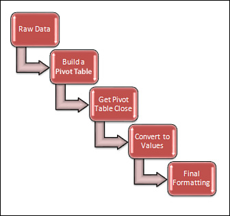
Figure 14.8 illustrates a typical pivot table experience. In this case, you should start with raw data. Produce a pivot table and use all sorts of advanced pivot table tricks to get it close. Convert the pivot table to values and do the final formatting in regular Excel.

Figure 14.8 Typical pivot table process.

The new method introduced by Rob Collie and described in the rest of this chapter puts a different spin on this. In this method, you build an ugly pivot table. You do not care about the formatting of this pivot table. You then go through a one-time, relatively painful process of building a nicely formatted shell to hold your final report. You then use GetPivotData to populate the shell report quickly.

From then on, when you get new data, you simply put it on the data sheet, refresh the ugly pivot table, and print the shell report.

Figure 14.9 illustrates this process.

Figure 14.9 How people inside of Microsoft use pivot tables.

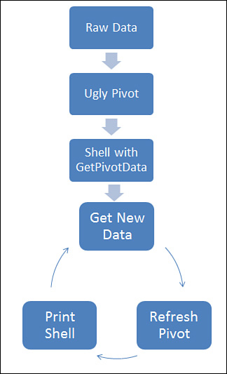
There are huge advantages to this method. For example, you do not have to worry about formatting the report after the first time. It comes much closer to an automated process.

The rest of this chapter walks you through the steps to build a dynamic report that shows actuals for months that have been completed and a forecast for future months.

Build an Ugly Pivot Table

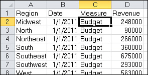
You have transactional data showing budget and actuals for each region of a company. The budget data is at a monthly level. The actuals data is at a daily level. Budget data exists for the entire year. Actuals exist only for the months that have been completed. Figure 14.10 shows the original data set.

Figure 14.10 The original data includes budget and actuals.

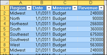
Because you will be updating this report every month, it makes the process easier if you have a pivot table data source that grows as you add new data to the bottom. While legacy versions of Excel would achieve this through a named dynamic range using the OFFSET function, you can do this in Excel 2010 by selecting one cell in your data and pressing Ctrl+T. Click OK to confirm that your data has headers.

You now have a formatted data set, as shown in Figure 14.11.

Figure 14.11 Format as a table to enable the pivot source data to expand in future months.

Your next step is to create a pivot table that has every possible value needed in your final report. You learn that GetPivotData is powerful, but it can only return values that are visible in the actual pivot table. It cannot reach through to the pivot cache to calculate items that are not in the pivot table.

Create the pivot table by following these steps:

1. Select Insert, PivotTable, OK.

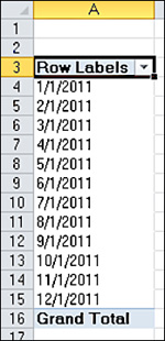
2. In the PivotTable Field List, select the Date field. Daily dates appear down the left side (see Figure 14.12).

Figure 14.12 Start with daily dates down the left.

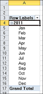
3. Select the first date cell in A4. From the PivotTable Options tab, select Group Field. Select Months and Years, as shown in Figure 14.13. Click OK. You now have actual month names down the left side, as shown in Figure 14.14.

Figure 14.13 Group the daily dates up to months and years.

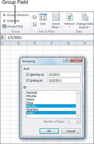
Figure 14.14 You have month names instead of dates.

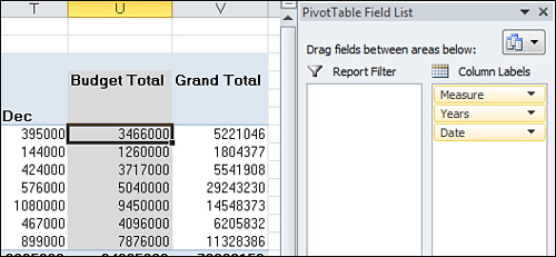
4. Drag the Years and Date field to the Column Labels drop zone in the Pivot Table Field List.

5. Drag Measure to the Column Labels drop zone.

6. Select Region to have it appear along the left column of the pivot table.

7. Select Revenue to have it appear in the Values area of the pivot table.

As shown in Figure 14.15, you now have one ugly pivot table. You might hate the words “Row Labels” and “Column Labels.” And having a total of January Actuals in Column B and January Budget in Column D is completely pointless. This is ugly. And for once, you do not care because no one other than you will ever see this pivot table.

Figure 14.15 The world’s ugliest pivot table.

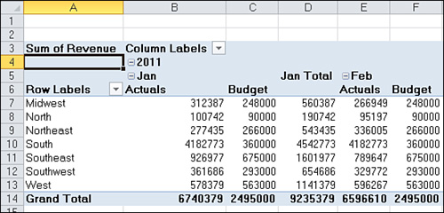
At this point, the goal is to have a pivot table with every possible data point that you could ever need in your final report. It is fine if the pivot table has extra data that you will never need in your report.

Build the Shell Report

Insert a blank worksheet in your workbook. Put away your pivot table hat and take out your straight Excel hat. You are going to use basic Excel formulas and formatting to create a nicely formatted report suitable for giving to your manager.

Follow these steps:

1. Put a report title in Cell A1.

2. Use the Cell Styles drop-down on the Home tab to format cell A1 as a Title.

3. Put a date in Cell A2 by using the formula =EOMONTH(TODAY(),0). This enters the serial number of the last day of the previous month in Cell B1. If you want to see how the formula is working, you can format the cell as a Date. If you are reading this on July 14, 2011, the date that appears in Cell B1 is June 30, 2011.

4. Select Cell A2. Press Ctrl+1 to go to Format Cells. On the Number tab, click Custom. Type a custom number format of Actuals Through mmmm/yyyy. This causes the calculated date to appear as text.

5. There is a chance that the text in Cell A2 is going to be wider than you want Column A to be. Select both Cells A2 and B2. Press Ctrl+1 to format cells. On the Alignment tab, select Merge Cells. This allows the formula in Cell A2 to spill over into B2 if necessary.

6. Type a Region heading in Cell A5.

7. Down the rest of Column A, type your region names. These names should match the names in the pivot table.

8. Where appropriate, add labels in Column A for Division totals.

9. Add a line for Total Company at the bottom of the report.

10. Month names stretch from Cells B4:M4. Enter this formula in Cell B4: =DATE(YEAR($A$2),COLUMN(A1),1).

11. Select Cell B4. Press Ctrl+1 to Format Cells. On the Number tab, select Custom and type a custom number format of MMM.

12. Right-justify Cell B4. Use the Cell Styles drop-down to select Heading 4.

13. Copy Cell B4 to Cells C4:M4. You now have true dates across the top that appear as month labels.

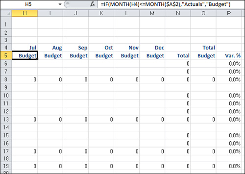
14. Enter this formula in Cell B5: =IF(MONTH(B4)<=MONTH($A$2),”Actuals”,”Budget”). Right-justify Cell B5. Copy across to Cells C5:M5. This should provide the word Actuals for past months, but the word Budget for future months.

15. Add a Total column heading in Cell N5. Add a Total Budget column in Cell O5. Enter Var % in Cell P5.

16. Fill in the regular Excel formulas necessary to provide division totals, the total company row, the grand total column, and the variance % column. For example:

• =SUM(B6:B7) in Cell B8 and copy across

• =SUM(B6:M6) in Cell N6 and copy down

• =IFERROR((N6/O6)-1,0) in Cell P6 and copy down

• =SUM(B10:B12) in Cell B13 and copy across

• =SUM(B15:B16) in Cell B17 and copy across

• =SUM(B6:B18)/2 in Cell B19 and copy across

17. Apply Heading 4 cell style to the labels in Column A and the headings in Rows 4:5.

18. Apply #,##0 number format to Cells B6:O19.

19. Apply 0.0% number format to Column P.

You now have a completed shell report, as shown in Figure 14.16 and Figure 14.17. This report has all the necessary formatting as desired by your manager. It has totals that add up the numbers that eventually come from the pivot table.

Figure 14.16 The left side of the shell report.

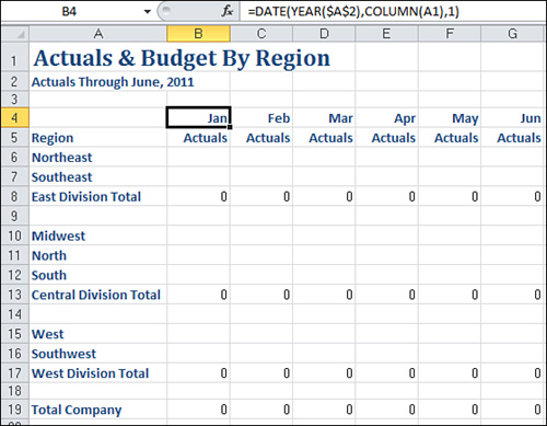
Figure 14.17 The right side of the shell report. Any place with a zero is a regular Excel formula.

In the next section, you use GetPivotData to complete the report.

Using GetPivotData to Populate the Shell Report

At this point, you are ready to take advantage of the thing that has been driving you crazy for years—that crazy Generate GetPivotData setting.

If you have ever cleared the setting back in Figure 14.7, go in and select this again. When it is selected, you see a checkmark next to Generate GetPivotData.

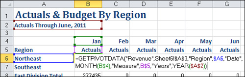
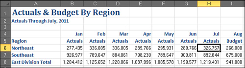
Go to Cell B6 on the shell report. This is the cell for Northeast region, January, Actuals.

1. Type = (equal sign) to start a formula (see Figure 14.18).

Figure 14.18 Start a formula on the shell report.

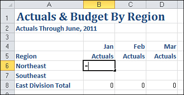
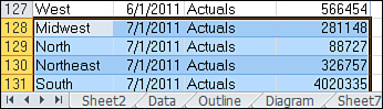
2. Move to the pivot table worksheet and click the cell for Northeast, January, Actuals. In Figure 14.19, this is Cell B9.

Figure 14.19 Using the mouse, click the correct cell in the pivot table.

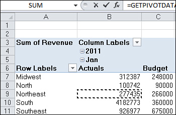
3. Press Enter to return to the shell report and complete the formula. Excel adds a GetPivotData function in Cell B6.

The formula says that the Northeast region actuals are $277,435.

The initial formula is =GETPIVOTDATA(“Revenue”,Sheet6!$A$3,“Region”,“Northeast”,“Date”,1,“Measure”,“Actuals”,“Years”,2011).

After years of ignoring the GetPivotData formula, you need to look at this monster formula closely to understand what it is doing. Figure 14.20 shows the formula in edit mode, along with the formula tool tip.

Figure 14.20 The GetPivotData formula generated by Microsoft.

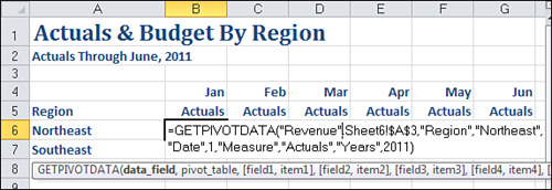
Here are the arguments in the formula:

• Data Field—This is the field in the Value area of the pivot table. Note that you use Revenue, not Sum of Revenue.

• Pivot Table—This is Microsoft’s way of asking, “Which pivot table do you mean?” All you have to do here is point to one single cell within the pivot table. The entry of Sheet6!$A$3 is the first populated cell in the pivot table. You are free to choose any cell in the pivot table that you want. However, because it does not matter which cell you choose, don’t worry about getting clever here. Leave the formula pointing to $A$3, and you will be fine.

• Field 1, Item 1—The formula generated by Microsoft shows Region as the field name and Northeast as the item value. Aha! So this is why the GetPivotData formulas that Microsoft generates cannot be copied. They are essentially hard-coded to point to one specific value. You want your formula to change as you copy it through your report. Edit the formula to change Northeast to $A6. By using only a single dollar sign before the A, you are enabling the row portion of the reference to vary as you copy the formula down.

• Field 2, Item 2—The next two pairs of arguments specify the Date field should be a 1. When the original pivot table was grouped by month and year, the month field retains the original field name of Date. The value for month is 1, which means January. You probably thought I was insane to build that outrageous formula and custom number format in Cell B4. That formula becomes useful now. Instead of hard coding a 1, use MONTH(B$4). Again, the single dollar sign before Row 4 indicates that the formula can get data from other months as it is copied across, but it should always reach back up to Row 4 as it is copied down.

• Field 3, Item 3—The field name is Measure and the item is Actuals. This happens to be correct for January, but when you get to future months, you want the measure to switch to Budget. Change the hard-coded Actuals to point to B$5.

• Field 4, Item 4—This is Years and 2011. I was almost ready to leave this one alone because it would be months before we have a new year. However, why not change the 2011 to YEAR($A$2)?

The new formula is shown in Figure 14.21. Rather than a formula that is hard-coded to work with only one value, you have created a formula that can be copied throughout the data set.

Figure 14.21 After editing, the GetPivotData formula is suitable for copying.

When you press Enter, you have the exact same answer that you had before editing the formula (see Figure 14.22). Compare this with the number you jotted down earlier to make sure.

Figure 14.22 The result of the edited formula should match the result before editing.

The edited formula is =GETPIVOTDATA(“Revenue”,Sheet6!$A$3,“Region”,$A6,“Date”,MONTH(B$4),“Measure”,B$5,“Years”,YEAR($A$2)).

Copy this formula to all the blank calculation cells in Columns B:M. Do not copy the formula to Column O yet.

Now that you have real numbers in the report, you might have to adjust some column widths.

The GetPivotData formula for the months can be tweaked to get the total budget. If you copy one formula to Cell O6, you get a #REF! error because the word Total in Cell O4 does not evaluate to a month.

Edit the formula to the pairs of arguments for Month and Years. You still have an error.

For GetPivotData to work, the number you are looking for must be in the pivot table. Because the original pivot table had Measure as the third column field, there is no actual column for Budget total.

Move the Measure field to be the first Column field, as shown in Figure 14.23.

Figure 14.23 Tweak the layout of the Column Labels fields so you have a Budget Total column.

When you return to the shell report, you find that the Total Budget formula in Cell O6 is now working fine (see Figure 14.24). Copy that formula down to the other blank data cells in Column O (see Figure 14.25).

Figure 14.24 After rearranging the pivot table, you have a working formula for Total Budget.

Figure 14.25 Copy the formula down to other cells in the Budget column to finish the report.

The formula in O6 is =GETPIVOTDATA(“Revenue”,Sheet6!$A$3,“Region”,$A6, “Measure”,O$5).

You now have a nicely formatted shell report that grabs values from a live pivot table. It certainly took more time to set up this report for the first month that you have to produce it, but it will be a breeze to update the report in future months.

To see the shell report in action, search for Pivot Table Data Crunching 14 at YouTube.

Updating the Report in Future Months

In future months, you can update your report by following these steps:

1. Paste actuals for the new month just below the original data set. Because the original data set is a Table, the table formatting automatically extends to the new rows. The pivot table source definition also extends (see Figure 14.26).

Figure 14.26 Copy new data below the old data.

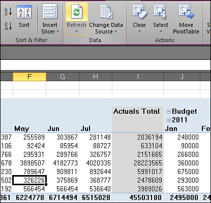
2. Go to the pivot table. Click the Refresh button on the Options tab (see Figure 14.27). The shape of the pivot table changes, but you do not care.

Figure 14.27 Refresh the pivot table.

3. Go to the shell report. In real life, you are done, but to test it, enter a date in Cell B2 such as 8/30/2011.

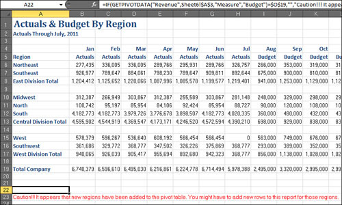
This process is so simple, that you will probably forget about the pain that you used to endure to create these monthly reports. The one risk is that a company reorg will add new regions to the pivot table. To be sure that your formulas are still working, add a small check section outside of the print range of the report. This formula in Cell A22 checks to see if the budget total calculated in Cell O19 matches the budget total back in the pivot table. Here is the formula:

=IF(GETPIVOTDATA(“Revenue”,Sheet6!$A$3,“Measure”,“Budget”)=$O$19,“”,“Caution!!! It appears that new regions have been added to the pivot table. You might have to add new rows to this report for those regions.”

In case the new region comes from a misspelling in the actuals, this formula checks the YTD actuals against the pivot table. Enter the following formula in Cell A23:

=IF(SUMIF(B5:M5,“Actuals”,B19:M19)=GETPIVOTDATA(“Revenue”,Sheet6!$A$3,“Measure”,“Actuals”),“”,“Caution!!! It appears that new regions have been added to the pivot table. You might have to add new rows to this report for those regions.”)

Change the font color of both of those cells to be red. You do not even notice them down there until something goes wrong, as shown in Figure 14.29.

Figure 14.29 Formulas in a check section monitor the calculated totals and the pivot totals to see if a new region appeared.

I thought that I would never write these words: GetPivotData is the greatest thing ever. How could we ever live without it?

Next Steps

The appendix is for those of you who have upgraded directly from Excel 2003 (or earlier) to Excel 2010. By the way, kudos for skipping Excel 2007! The appendix assists you in finding old pivot table commands on the Excel 2010 ribbon.