Chapter 1
The Basics
Before we get into the “Mastering” of the AutoCAD® Civil 3D® program, it is important to understand the basics. There are numerous dialogs, Ribbons, menus, and icons to pore over. They might seem daunting at first glance, but as you use them, you will gain familiarity with their location and use. In this chapter, you will explore the interface and learn terminology that will be used throughout this book.
In addition, we will introduce the Lines and Curves commands, which offer a plethora of options for drawing lines and curves accurately.
In this chapter, you will learn to:
- Find any Civil 3D object with just a few clicks
- Modify the drawing scale and default object layers
- Navigate the Ribbon's contextual tabs
- Create a curve tangent to the end of a line
- Label lines and curves
The Interface
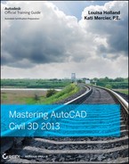
If you have used Civil 3D 2010 or newer, the interface for Civil 3D 2013 is basically the same. If you are new to Civil 3D or are coming from Civil 3D 2009 or prior, this part of the chapter is for you. Civil 3D uses a Ribbon-based interface, which is where you will access many of the tools. The Ribbon consists of tabs and panels that organize tools into logical groups. When working in Civil 3D 2013, you will spend the majority of your time on the Home tab, shown in Figure 1.1.
Figure 1.1 The Ribbon runs horizontally across the top of your screen and is where you will access many tools.
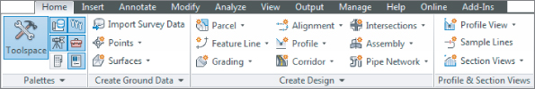
The interface may change slightly, depending on what task you are performing. When you click on a Civil 3D object, you will see a context-specific contextual tab appear in the Ribbon. Figure 1.2 shows the Civil 3D palette sets, along with the AutoCAD tool palettes and Ribbon displayed in a typical environment.
Figure 1.2 Overview of the Civil 3D environment. Toolspace is docked to the left, and tool palettes float over the drawing window. The Ribbon is at the top of the workspace.
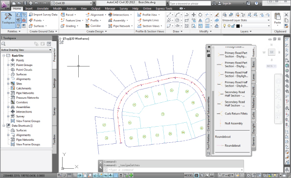
Panels are subgroups within each tab that further organize your tools. For example, the Palettes panel on the Home tab (shown in Figure 1.3) is where you can toggle on or off the elements you are about to learn.
Figure 1.3 Palettes panel of the Home tab
Toolspace
![]()
Toolspace is a set of palettes that is specific to Civil 3D. You will want to have the palette visible any time you are working in Civil 3D. If you do not see it, click the Toolspace button on the Home tab and select Palettes.
Toolspace can have as many as four tabs to manage user data, as follows:
- Prospector
- Settings
- Survey
- Toolbox
The tabs can be turned on or off by toggling the display on the Palettes panel.
Each tab has a unique role to play in working with Civil 3D. Prospector and Settings will be your most frequently visited tabs. Survey and Toolbox are used for special tasks that you will examine in the following section.
Prospector
Prospector shows your drawing-specific information about what currently exists in your project. Civil 3D objects are listed in workflow order, starting at the top of the listing. Each main grouping under the drawing name is referred to as a collection. If you expand a collection by clicking on the plus sign next to the name, you will see the contents of that group. Some of these groups are empty until objects are created.
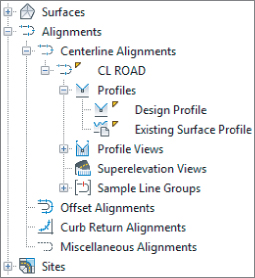
Because all Civil 3D data is dynamically linked together, you will see object dependencies as well. You can learn details about an individual object by expanding the tree and selecting an object (Figure 1.4).
Figure 1.4 A look at the Alignment branch of the Prospector tab. Profiles are linked to alignments; therefore, they appear under alignments.
Right-clicking the collection name allows you to select various commands that apply to all the members of that collection. For example, right-clicking the Point Groups collection brings up the menu shown in Figure 1.5.
Figure 1.5 Context-sensitive menus in Prospector
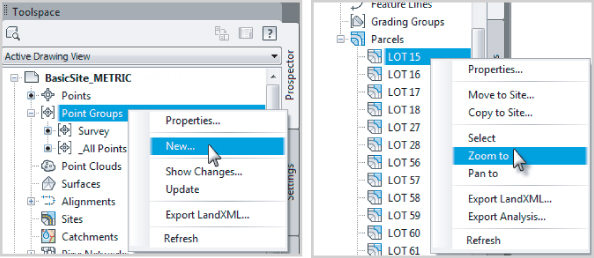
In addition, right-clicking the individual object in the list view offers many commands unique to Civil 3D: Zoom To Object and Pan To Object are typically included. By using these commands, you can find any parcel, point, cross section, or other Civil 3D object in your drawing almost instantly.
For example, if you are interested in locating LOT 27 using the Zoom To command, locate the Sites collection on the Prospector tab of Toolspace. Expand the Proposed Site and highlight Parcels. At the bottom of Prospector, you will see all the lots listed. To locate LOT 27 graphically, right-click it and select Zoom To.
Near the top of the Toolspace you will see a pull-down giving you the option of Active Drawing View or Master View.
Active Drawing view will show you:
- The current drawing
- Data shortcuts
Master view will show you:
- Open drawings
- Data shortcuts
- Drawing templates
Master view will list every drawing you have open, as well as its contents and templates. If you use Master view, the name of the drawing you are working with appears at the top of the list in bold. To make a drawing current, right-click its name in Prospector and select Switch To.
Many users prefer to use the Active Drawing view. You can have more than one drawing open, but Prospector displays only one set of Civil 3D data at a time. Active Drawing view will change to reflect whichever drawing is current.
In addition to the branches, Prospector has a series of icons across the top that toggle various settings on and off. Some of the Civil 3D icons from previous versions have been removed, and their functionality has been universally enabled for Civil 3D 2013. Let's take a closer look at those icons:
![]()
Item Preview Toggle
Turns on and off the display of the Toolspace item preview within Prospector. These previews can be helpful when you're navigating drawings in projects (you can select one to check out), or when you're attempting to locate a parcel on the basis of its visual shape. In general, however, you can turn off this toggle — it's purely a user preference.
![]()
Preview Area Display Toggle
When Toolspace is undocked, this button moves the preview area from the right of the tree view to beneath the tree view area.
![]()
Panorama Display Toggle
Turns on and off the display of the Panorama window (which we'll discuss in a bit). To be honest, there doesn't seem to be a point to this button, but it's here nonetheless.
![]()
Help
Don't underestimate how helpful Help can be!
As you navigate the tabs of Toolspace, you will encounter many symbols to help you along the way. Table 1.1 shows you a few that you should familiarize yourself with.
Table 1.1 Common Toolspace symbols and meanings
| Symbol | meaning |
|
|
The object or style is in use. |
|
|
Clicking this will expand the branch of Toolspace. |
|
|
Clicking this will collapse the branch of Toolspace. |
|
|
Data resides in this branch and more information can be found at the bottom of Toolspace. |
|
|
Object needs to be rebuilt or updated. Can also indicate broken data reference. |
Settings
The Settings tab of Toolspace controls all things aesthetic and the default behavior of the commands. Text placed by Civil 3D is controlled by label styles. Object styles control the look of design elements such as surface contours or pipes. The bulk of these settings and styles should be set in your template drawing. Every time you start a project with your company's Civil 3D–specific template, items such as an alignment's color and linetype will already be set. Chapter 20, “Label Styles,” and Chapter 21, “Object Styles,” are dedicated to building these styles. Later on in this chapter you will learn more about templates.
Drawing Settings
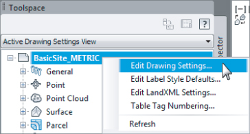
At the top of the Settings tab you will see the name of the drawing. There are some important settings you need to locate before proceeding with a project. Right-click on the name of the drawing and click Edit Drawing Settings to access the Drawing Settings dialog, shown in Figure 1.6.
Figure 1.6 Accessing the Drawing Settings dialog
Try this quick exercise to make sure you know how to get into the drawing settings:
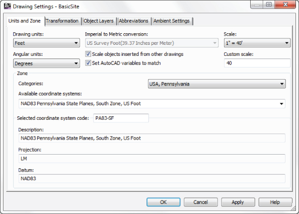
Figure 1.7 Before placing any project-specific information in the drawing, set the coordinate system in the Units And Zone tab of the Drawing Settings.
Each tab in this dialog controls a different aspect of the drawing. Most of the time, you'll pick up the Object Layers, Abbreviations, and Ambient Settings from a company-wide template. However, the drawing scale and coordinate information change for every job, so you'll visit the Units And Zone and Transformation tabs frequently.
Units And Zone Tab
The Units And Zone tab lets you specify metric or Imperial units for your drawing. You can also specify the conversion factor between systems. If you choose a coordinate system with International or US Foot specified, this setting will become unavailable.
This tab also includes the options Scale Objects Inserted From Other Drawings and Set AutoCAD Variables To Match. The Set AutoCAD Variables To Match option sets the base AutoCAD angular units, linear units, block insertion units, hatch pattern, and linetype units to match the values placed in this dialog. As shown in Figure 1.7, you do want these options selected.
The scale that you see on the right side of the Units And Zone tab is the same as your annotation scale. You can change it here, but it is much easier to select your annotation scale from the bottom of the drawing window.
If you choose to work in assumed coordinates, you can leave Zone set to No Datum, No Projection. To set the coordinate system for your locale, first set the category from the long list of possibilities. Civil 3D is a worldwide product; therefore, most recognized surveying coordinate systems (including obsolete ones) can be found in the options. Once your coordinate system has been established, you can change it on the Transformation tab if desired.
Try the following quick exercise, working in the drawing from the previous exercise, to practice setting a drawing coordinate system:
Transformation Tab
Earth is neither flat nor a perfect sphere. In reality, Earth is more of a squashed sphere, wider at the equator than at the poles. The mathematical approximation of Earth's physical shape is called an ellipsoid. The ellipsoid is constantly being fine-tuned to increase accuracy for precise geographic modeling. To make matters even more complicated, the gravitational pull of Earth is not distributed evenly, creating a slight skew between what a surveyor measures and how it relates to the ellipsoid. The gravitational representation of Earth is referred to as the geoid.
Luckily, most engineers and surveyors do not need to worry about all this. Most survey-grade GPS equipment takes care of the transformation to local grid coordinates for you. In the United States, state plane coordinate systems already have regional projections taken into account. In the rare case that surveyors need to transform local observations from geoid to ellipsoid, and ellipsoid to grid manually, the Transformation tab makes the computation quickly.
With a base coordinate system selected, you can do any further refinement you'd like using the Transformation tab, shown in Figure 1.8. The coordinate systems on the Units And Zone tab can be refined to meet local ordinances, tie in with historical data, complete a grid to ground transformation, or account for minor changes in coordinate system methodology. These changes can include the following:
Figure 1.8 The Transformation tab
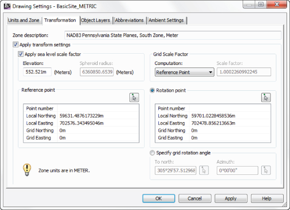
Apply Sea Level Scale Factor
This value is known in some circles as elevation factor or orthometric height scale. Sea Level Factor takes into account the mean elevation of the site and the spheroid radius that is currently being applied as a function of the selected zone ellipsoid.
Grid Scale Factor
At any given point on a projected map, there is a distortion between the “flat” measurement and the measurement on the ellipsoid. Grid Scale Factor is based on a 1:1 value, a user-defined uniform scale factor, a reference point scaling, or a prismoidal transformation in which every point in the grid is adjusted by a unique amount.
Reference Point
To apply Grid Scale Factor and Sea Level Factor correctly, you need to tell Civil 3D where you are on Earth. Reference Point can be used to set a singular point in the drawing field via pick or point number, local northing and easting, or grid northing and easting values.
Rotation Point
Rotation Point can be used to set the reference point for rotation via the same methods as the reference point.
Specify Grid Rotation Angle
Some people may know this as the convergence angle. This is the angle between Grid North and True North. Enter an amount or set a line to north by picking an angle or deflection in the drawing. You can use this same method to set the azimuth if desired.
Most engineering firms work on either a defined coordinate system or an arbitrary system, so none of these changes are necessary. Given that, this tab will be your only method of achieving the necessary transformation for certain surveying and geographic information system (GIS)-based and land surveying–based tasks. It should be noted that this is not the place to transform assumed coordinates to a predefined coordinate system. See Chapter 2, “Survey,” to learn how to translate a survey.
Object Layers
Civil 3D and AutoCAD layers have a love–hate relationship with each other. Civil 3D is built on top of AutoCAD; therefore, all the objects do reside on layers. However, Civil 3D is not traditional CAD. Your surfaces, corridors, points, profiles, and everything else generated by Civil 3D are dynamic objects rather than simple lines, arcs, or circles.
When you create an alignment in Chapter 6, “Alignments,” for example, you will not have to think about the current layer. This is because Civil 3D styles “push” objects and labels to the correct layer as part of their intelligence.
Layers are found in several areas of the Civil 3D template. The first location you will examine is the layers found in the Drawing Settings area. The layers listed here represent overall layers where the objects will be created. For those of you who are familiar with AutoCAD blocks, it is useful to think of these layers in the same way as a block's insertion layer.
In the Object Layers tab, every Civil 3D object must have a layer set, as shown in Figure 1.9. Do not leave any object layers set to 0. An optional modifier can be added to the beginning (prefix) or end (suffix) of the layer name to further separate items of the same type.
Figure 1.9 Every object is on a layer; the corridor layer contains a modifier.

A common practice is to add wildcard suffixes to corridor, surface, pipe, and structure layers to make it easier to manipulate them separately. For example, if the layer for a corridor is specified to be C-ROAD-CORR and a suffix of -* (dash asterisk, as shown in Figure 1.9) is added as the modifier value, a new layer will automatically be created when a new corridor is created. The resulting layer will take on the name of the corridor. If the corridor is called 13th Street, the new layer name will be C-ROAD-CORR-13th Street. This new layer is created once and is not dynamic to the object name. In other words, if you decide to rename “13th Street” to “Stephen Colbert Street,” the layer remains C-ROAD-CORR-13th Street.
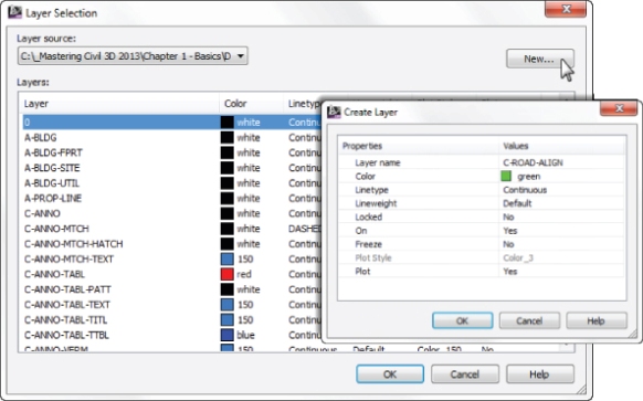
If the main layer name you are after does not exist in the drawing, you can create it as you work through the Object Layers dialog. Click the New button, as shown in Figure 1.10, and set up the layer as needed including Color, Lineweight, Linetype, and so forth.
Figure 1.10 Click New to add a new layer.
“Immediate And Independent Layer On/Off Control Of Display Components” is a setting you will want to have selected. As mentioned earlier, the layers listed here are like an object's insertion layer. However, you will encounter more layers within the object's display style (these are the object styles you will learn about in Chapter 21). Having this option selected allows you to turn off components within an object's style without turning off the entire object. For example, consider a surface whose Object Layer is set as C-TOPO. When that surface has contours displayed, the major contours might be on C-TOPO-MAJR and the minor contours may be on C-TOPO-MINR. With this option selected, you could turn off the C-TOPO-MINR independent from the overall object.
In the following exercise, you set object layers in a template:
- For Pipe, create a layer called C-NTWK-PIPE with a Modifier of Suffix and a Value of -*.
- For Pipe-Labeling, create a new layer called C-NTWK-PIPE-TEXT.
- For Pipe And Structure Table, set the layer to C-NTWK-PIPE-TABL.
- For Pipe Network Section, create a new layer called C-NTWK-XSEC.
- For Pipe Network Profile, create a new layer called C-NTWK-PROF.
Figure 1.11 Examples of the completed layer names in the Object Layers tab

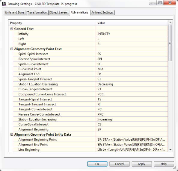
Abbreviations
When you add labels to certain objects, Civil 3D automatically uses the abbreviations from this area to indicate geometry features. For example, left is L and right is R.
Civil 3D uses industry-standard abbreviations wherever they are found. If necessary, you can easily change VPI to PVI for Point of Vertical Intersection. In most cases, changing an abbreviation is as simple as clicking in the Value field and typing a new one. Notice that the Alignment Geometry Point Entity Data section has a larger set of values and some special coding attached (as shown toward the bottom of Figure 1.12). These are more representative of other label styles. You will visit the Text Component Editor in Chapter 20.
Figure 1.12 Customizable down to the letter, the Abbreviations tab
Ambient Settings
Examine the settings in the Ambient Settings tab to see what can be set here. The main options you'll want to adjust are in the General category and the display precision in the subsequent categories.
The precision that you see in this dialog does not change the label precision. The precision you see here is the number of decimal places reported to you in various dialogs.
Being familiar with the way this tab works will help you further down the line, because almost every other settings dialog in the program works like the one shown in Figure 1.13.
Figure 1.13 Ambient Settings at the main drawing level

Plotted Unit Display Type
Civil 3D knows you want to plot at the end of the day. In this case, it's asking how you would like your plotted units measured. For example, would you like that bit of text to be 0.25″ tall or 1/4″ high? Most engineers are comfortable with the Leroy method of text heights (L80, L100, L140, and so on), so the decimal option is the default.
Set AutoCAD Units
This option specifies whether Civil 3D should attempt to match AutoCAD drawing units, as specified on the Units And Zone tab.
Save Command Changes To Settings
Set this to Yes. This setting is incredibly powerful but a secret to almost everyone. By setting it to Yes, you ensure that your changes to commands will be remembered from use to use. This means if you make changes to a command during use, the next time you call that Civil 3D command, you won't have to make the same changes. It's frustrating to do work over because you forgot to change one of the five things that needed changing, so this setting is invaluable.
Show Event Viewer
Event Viewer is the main Civil 3D feedback mechanism, especially when things go wrong. Event Viewer uses the Panorama interface to display warnings such as when a surface contains crossing breaklines. Event viewer will pop up with informational messages as well. If you have multiple monitors, it is a good idea to leave Panorama on but set aside for review.
Show Tooltips
One of the cool features that people remark on when they first use Civil 3D is the small pop-up that displays relevant design information when the cursor is paused on the screen. This includes things such as station-offset information, surface elevation, section information, and so on. Once a drawing contains numerous bits of information, this display can be overwhelming; therefore, Civil 3D offers the option to turn off these tooltips universally with this setting. A better approach is to control the tooltips at the object type by editing the individual feature settings. You can also control the tooltips by pulling up the properties for any individual object and looking at the Information tab.
Imperial To Metric Conversion
This setting displays the conversion method specified on the Units And Zone tab. The two options are US Survey Foot and International Foot.
New Entity Tooltip State
This setting controls whether the tooltip is turned on at the object level for new Civil 3D objects. If you change this setting to Off partway through a project, the tooltip will not be displayed for any Civil 3D objects created after the change.
Driving Direction
Specifies the side of the road that forward-moving vehicles use for travel. This setting is important in terms of curb returns and intersection design.
Drawing Unit, Drawing Scale, and Scale Inserted Objects
These settings were specified on the Units And Zone tab but are displayed here for reference, and so that you can lock them if desired.
Independent Layer On
This is the same control that was set on the Object Layers tab. Yes is the recommended setting, as described previously.
The Ambient Settings for Direction offer the following choices:
- Unit: Degree, Radian, and Grad.
- Precision: 0 through 8 decimal places.
- Rounding: Round Normal, Round Up, and Truncate.
- Format: Decimal, two types of DDMMSS, and Decimal DMS. In most cases, people want to display DD°MM?SS.SS?. Whether you want spaces between the subdivisions is up to you.
- Direction: Short Name (spaced or unspaced) and Long Name (spaced or unspaced).
- Capitalization: you can display as typed, or force uppercase, lowercase, or title caps.
- Sign: gives you your choice of how negative numbers are displayed. You can use a negative sign to denote negative numbers only, use a parenthesis to denote a negative, or use a sign regardless of value. The latter option will show a plus for positive values and a minus for negative values.
- Measurement Type: Bearings, North Azimuth, and South Azimuth.
- Bearing Quadrant: This should be left at the industry standard. 1 - NE, 2-SE, 3 - SW, 4-NW.
![]()
When you're using the Bearing Distance transparent command, for example, these settings control how you input your quadrant, your bearing, and the number of decimal places in your distance.
Explore the other categories, such as Angle, Lat Long, and Coordinate, and customize the settings to how you work.
At the bottom of the Ambient Settings tab is a Transparent Commands category. These settings control how (or if) you're prompted for the following information:
Prompt For 3D Points
Controls whether you're asked to provide a z elevation after x and y have been located.
Prompt For Y Before X
For transparent commands that require x and y values, this setting controls whether you're prompted for the y-coordinate before the x-coordinate. Most users prefer this value set to False so they're prompted for an x-coordinate and then a y-coordinate.
Prompt For Easting Then Northing
For transparent commands that require Northing and Easting values, this setting controls whether you're prompted for the Easting first and the Northing second. Most users prefer this value set to False, so they're prompted for Northing first and then Easting.
Prompt For Longitude Then Latitude
For transparent commands that require longitude and latitude values, this setting controls whether you're prompted for Longitude first and Latitude second. Most users prefer this set to False, so they're prompted for Latitude and then Longitude.
The settings that are applied here can also be changed at the object levels. For example, you may typically want elevation to be shown to two decimal places, but when looking at surface elevations, you might want just one. The Override and Child Override columns give you feedback about these types of changes. See Figure 1.14.
Figure 1.14 The Child Override indicator in the Time, Distance, and Elevation values

The Override column shows whether the current setting is overriding something higher up. Because you're at the Drawing Settings level, these are clear. However, the Child Override column displays a down arrow, indicating that one of the objects in the drawing has overridden this setting. After a little investigation of the objects, you'll find the override in the Edit Feature Settings of the Profile view, as shown in Figure 1.15.
Figure 1.15 The Profile Elevation Settings and the Override indicator
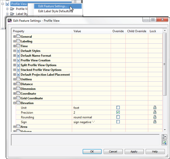
Notice that in this dialog, the box is checked in the Override column. This indicates that you're overriding the settings mentioned earlier, and it's a good alert that things have changed from the general Drawing Settings to this Object Level setting.
But what if you don't want to allow those changes? Each Settings dialog includes one more column: Lock. At any level, you can lock a setting, graying it out for lower levels. This can be handy for keeping users from changing settings at the lower level that perhaps should be changed at a drawing level, such as sign or rounding methods.
Survey
The Survey palette is displayed optionally and controls the use of the survey, equipment, and figure prefix databases. Survey is an essential part of land-development projects. Because of the complex nature of this tab, all of Chapter 2 is devoted to it.
Toolbox
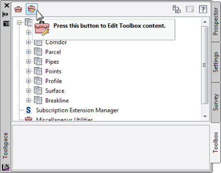
The Toolbox is a launching point for add-ons and reporting functions. To access the Toolbox, from the Home tab in the Ribbon, select Toolspace ⇒ Palettes and click the Toolbox icon (as shown previously in Figure 1.3). Out of the box, the Toolbox contains reports created by Autodesk, but you can expand its functionality to include your own macros or reports. The buttons on the top of the Toolbox, shown in Figure 1.16, allow you to customize the report settings and add new content. If you are an Autodesk Subscription customer, new goodies released throughout the year are frequently accessed from this area.
Figure 1.16 The Toolbox with the Edit Toolbox Content icon highlighted
Panorama
The Panorama window is the Civil 3D feedback and tabular editing mechanism. It's designed to be a common interface for a number of different Civil 3D–related tasks, and you can use it to provide information about the creation of profile views, to edit pipe or structure information, or to run basic volume analysis between two surfaces. For an example of Panorama in action, open it up by going to the Home tab ⇒ Palettes Panel flyout and clicking on the Event Viewer icon. You'll explore and use Panorama more during this book's discussion of specific objects and tasks.
Ribbon
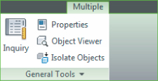
As with AutoCAD, the Ribbon is the primary interface for accessing Civil 3D commands and features. When you select an AutoCAD Civil 3D object, the Ribbon displays commands and features related to that object in a contextual tab. If several object types are selected, the Multiple contextual tab is displayed. Use the following procedure to familiarize yourself with the Ribbon:
Figure 1.17 The contextual tab in the Ribbon

Figure 1.18 When more than one object is selected, the Multiple tab appears.
Civil 3D Templates
Styles and settings should come from your template. Ideally, that template will have all the styles you need for the type of project you are working on. If you find you are constantly changing style settings, reexamine your workflow.
When starting a project, or continuing a project from an outside source, it is important to start with a Civil 3D template file. Right after installing the software you will see two usable Civil 3D–specific templates (Figure 1.19).
Figure 1.19 Civil 3D template

The Civil 3D–specific templates are:
- _AutoCAD Civil 3D (Imperial) NCS.dwt
- _AutoCAD Civil 3D (Metric) NCS.dwt
Starting New Projects
When you start a project with the correct template (DWT file), the repetitive task of defining the basic framework for your drawing is already completed. As you know, a base AutoCAD DWT file contains the following:
- Unit type (architectural or decimal) and insertion scale (meters or feet)
- Layers and their respective linetypes, colors, and other properties
- Text styles
- Dimension and multileader styles
- Layouts and plot setups
- Block definitions
Civil 3D takes the base AutoCAD template and kicks it up several notches. In addition to the items just listed, a Civil 3D template contains the following:
- More specific unit information (international feet, survey feet, or meters)
- Civil object layers
- Ambient Settings
- Label styles and formulas (expressions)
- Object styles
- Command settings
- Object naming templates
- Report settings
- Description key sets
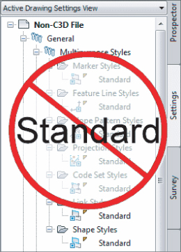
You must always start new projects with a proper Civil 3D template. If you receive a drawing from a non–Civil 3D user and need to continue it in Civil 3D, you must import the styles and settings. Without suitable styles and settings, all of your object and label styles will show up with the name Standard, as shown in Figure 1.20. You do not want objects and labels to use the Standard style, as it is the Civil 3D equivalent of drawing on layer 0. Items that use the Standard style appear on layer 0, and will contain the most basic display settings.
Figure 1.20 A non–Civil 3D DWG will list all styles as Standard, which is the Civil 3D equivalent to drawing on layer 0.
![]()
- The Insert command will detect the units of the incoming drawing and scale it to match your drawing.
- If both drawings have a coordinate system defined, Civil 3D will place the incoming drawing by geographic data.
- All of your styles and settings will stay intact, including a few items that do not get imported using the Import Styles command.
Importing Styles
![]()
Luckily, importing styles from an existing drawing or template has gotten much easier. You can find the Import Styles button on the Styles panel of the Manage tab in the Ribbon. When you click the button, you will be prompted to browse for the template (DWT) or drawing (DWG) that contains the styles you are looking for.
You must save the drawing before you can import styles. If you forget, you will be prompted to save the drawing before you can proceed with the import.
Once you select the file whose styles you will import, a dialog similar to Figure 1.21 appears.
Import Settings
Notice the Import Settings option at the bottom of the dialog. This option is turned on by default. As you look through the list of styles to be imported, you will notice that some items are grayed out and can't be modified.
The grayed-out styles represent items in command settings. Styles referred to in command settings must be imported if the Import Settings option is turned on. You will read about command settings in the upcoming section.
Uncheck Conflicting
You will also notice items with a warning symbol (see Basic in Figure 1.21). The warning symbol indicates there is a style in the current drawing with the same name as a style in the batch to be imported. Use the Uncheck Conflicting button if you do not want styles in the destination drawing to be overwritten. If you leave these items selected, the incoming styles “win.” If you are not sure if there is a difference between the styles, pause your cursor over the style name and a tooltip will tell you what (if any) difference exists.
Figure 1.21 Import Civil 3D Styles dialog

Uncheck Added
Use the Uncheck Added button if you only want styles with the same name to come in. Wherever possible, Civil 3D will release items in the To Be Added categories. In cases where a style is used by a setting, you will not be able to uncheck it unless you do not import settings.
Uncheck Deleted
A style in the current drawing will be deleted if the source drawing does not contain a style with the same name. Use the Uncheck Deleted button to prevent the style from being deleted.
Labeling Lines and Curves
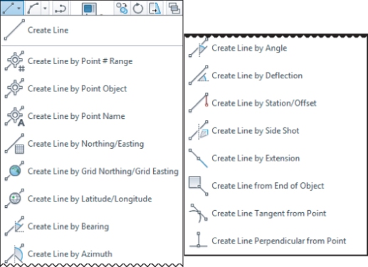
You can draw lines many ways in an AutoCAD-based environment. The tools found on the Draw panel of the Home tab in the Ribbon create lines that are the same as those created by the standard AutoCAD Line command. How the Civil 3D lines differ from those created by the regular Line command isn't in the resulting entity, but in the process of creating them. Figure 1.22 shows the available line commands.
Figure 1.22 Line creation tools
Later on in this chapter you will take a look at transparent commands. Transparent commands allow you to draw any object using similar “Civil-friendly” techniques.
Coordinate Line Commands
The next few commands discussed in this section help you create a line using Civil 3D points and/or coordinate inputs. Each command requires you to specify a Civil 3D point, a location in space, or a typed coordinate input. These Line tools are useful when your drawing includes Civil 3D points that will serve as a foundation for linework, such as the edge of pavement shots, wetlands lines, or any other points you'd like to connect with a line.
Create Line Command
The Create Line command on the Draw panel of the Home tab in the Ribbon issues the standard AutoCAD Line command. It's equivalent to typing line on the command line or, clicking the Line tool on the Draw toolbar.
Create Line By Point # Range Command
![]()
![]()
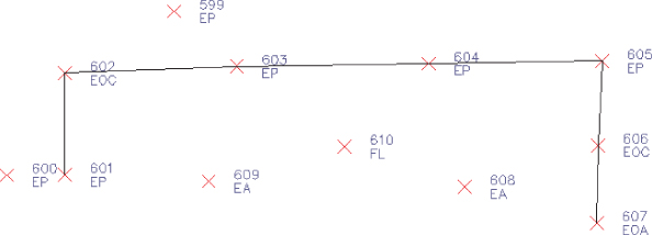
The Create Line By Point # Range command prompts you for a point number. You can type in an individual point number, press , and then type in another point number. A line is drawn connecting those two points. You can also type in a range of points, such as 601-607. Civil 3D draws a line that connects those lines in numerical order—from 601 to 607, and so on (see Figure 1.23). The line that is created by this method connects point-to-point regardless of the description of type of point.
Figure 1.23 A line created using 601-607 as input
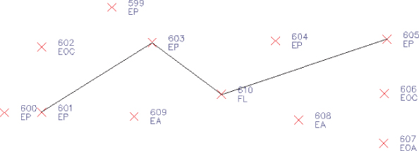
Alternatively, you can enter a list of points such as 601, 603, 610, 605 (Figure 1.24). Civil 3D draws a line that connects the point numbers in the order of input. This approach is useful when your points were taken in a zigzag pattern (as is commonly the case when cross-sectioning pavement), or when your points appear so far apart in the AutoCAD display that they can't be readily identified.
Figure 1.24 A line created using 601, 603, 610, 605 as input
Create Line By Point Object Command
![]()
The Create Line By Point Object command prompts you to select a point object. To select a point object, locate the desired start point and click any part of the point. This tool is similar to using the regular Line command and a Node object snap (also known as Osnap); however, it will only work on Civil 3D points.
Create Line By Point Name Command
![]()
![]()
The Create Line By Point Name command prompts you for a point name. A point name is a field in Point properties, not unlike the point number or description. The difference between a point name and a point description is that a point name must be unique. It is important to note that some survey instruments name points rather than number points as is the norm.
To use this command, enter the names of the points you want to connect with linework.
Create Line By Northing/Easting and Create Line By Grid Northing/ Easting Commands
![]()
![]()
The Create Line By Northing/Easting and Create Line By Grid Northing/Easting commands let you input northing (y) and easting (x) coordinates as endpoints for your linework. The Create Line By Grid Northing/Easting command requires that the drawing have an assigned coordinate system. This command can be useful when working with known surveyed points or features in a state plane coordinate system (SPCS).
Create Line By Latitude/Longitude Command
![]()
The Create Line By Latitude/Longitude command prompts you for geographic coordinates to use as endpoints for your linework. This command also requires that the drawing have an assigned coordinate system. For example, if your drawing has been assigned Delaware State Plane NAD83 US Feet and you execute this command, your Latitude/Longitude inputs are translated into the appropriate location in your state plane drawing. This command can be useful when you are drawing lines between waypoints collected with a standard handheld GPS unit.
Direction-Based Line Commands
The next few commands help you specify the direction of a line. Each of these commands requires you to choose a start point for your line before you can specify the line direction. You can specify your start point by physically choosing a location, using an Osnap, or using one of the point-related line commands discussed earlier.
Many of these line commands require a line or arc, and will not work with a polyline. Those commands include Create Line By Sideshot, Create Line By Extension, Create Line From End Of Object, Create Line Tangent From Point, and Create Line Perpendicular from Point.
Create Line By Bearing Command
![]()
The Create Line By Bearing command will likely be one of your most frequently used line commands.
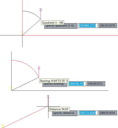
This command prompts you for a start point, followed by prompts to input the Quadrant, Bearing, and Distance values. You can enter values on the command line for each input, or you can graphically choose inputs by picking them on screen. The glyphs at each stage of input guide you in any graphical selections. After creating one line, you can continue drawing lines by bearing, or you can switch to any other method by clicking one of the other Line By commands on the Draw panel (see Figure 1.25).
Figure 1.25 The tooltips for a quadrant (top), a bearing (middle), and a distance (bottom)
Create Line By Azimuth Command
![]()
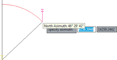
The Create Line By Azimuth command prompts you for a start point, followed by a north azimuth, and then a distance (Figure 1.26).
Figure 1.26 The tooltip for the Create Line By Azimuth command
Create Line By Angle Command
![]()
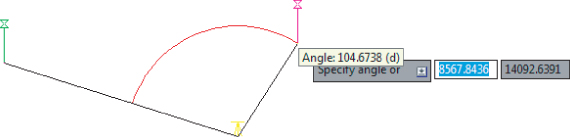
The Create Line By Angle command prompts you for a start point, and ending point (think backsight), a turned angle, and then a distance (Figure 1.27). This command is useful when you're creating linework from angles-right (in lieu of angles-left), and distances recorded in a traditional handwritten field book (required by law in many states).
Figure 1.27 The tooltip for the Create Line By Angle command
Create Line By Deflection Command
![]()
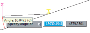
By definition, a deflection angle is the angle turned from the extension of a line from the backsight extending through an instrument. Although this isn't the most frequently used surveying tool in this day of data collectors and GPSs, on some occasions you may need to create this type of line. When you use the Create Line By Deflection command, the command line and tooltips prompt you for a deflection angle followed by a distance (Figure 1.28). In some cases, deflection angles are recorded in the field in lieu of right angles.
Figure 1.28 The tooltips for the Create Line By Deflection command
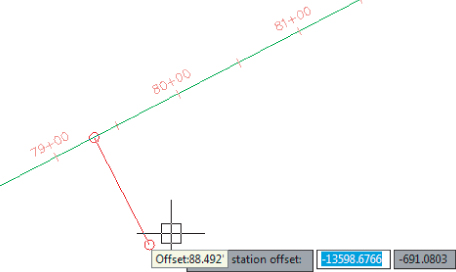
Create Line By Station/Offset Command
![]()
To use the Create Line By Station/Offset command, you must have a Civil 3D Alignment object in your drawing. The line created from this command allows you to start and/or end a line on the basis of a station and offset from an alignment.
You're prompted to choose the alignment and then input a station and offset value. The line begins at the station and offset value. On the basis of the tooltips, you might expect the line to be drawn from the alignment station at offset zero and out to the alignment station at the input offset. This isn't the case.
When prompted for the station, you're given a tooltip that tracks your position along the alignment, as shown in Figure 1.29. You can graphically choose a station location by picking in the drawing (including using your Osnaps to assist you in locking down the station of a specific feature). Alternatively, you can enter a station value on the command line.
Figure 1.29 The Create Line By Station/Offset command provides a tooltip for you to track stationing along the alignment.

Once you've selected the station, you're given a tooltip that is locked on that particular station and tracks your offset from the alignment (see Figure 1.30). You can graphically choose an offset by picking in the drawing, or you can type an offset value on the command line.
Figure 1.30 The Create Line By Station/Offset command provides a tooltip that helps you track the offset from the alignment.
Create Line By Side Shot Command
![]()
The Create Line By Side Shot command starts by asking you to select a line (or two points) that will be the basis for creating a new line. After you select the first line, you will see a yellow glyph indicating your occupied point (see Figure 1.31). By default, Civil 3D is looking for an angle-right and distance to establish the first point of the new line. However, you can follow the command prompts to change the angle entry to bearing, direction, or azimuth.
Figure 1.31 The tooltip for the Create Line By Side Shot command tracks the angle, bearing, deflection, or azimuth of the side shot.

Once you have entered data for the first point, you will be asked a second time for an angle and a distance to place the second point of the new line.
The occupied point represents the setup of your surveying station, whereas the direction to the end point of the first line represents your surveying backsight. This tool may be most useful when you're creating stakeout information or re-creating data from field notes. If you know where your crew set up and you have their side-shot angle measurements, but you don't have electronic information to download, this tool can help.
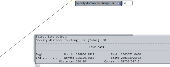
Create Line By Extension Command
![]()
The Create Line By Extension command is similar to the AutoCAD Lengthen command. This command allows you to add length to a line or specify a desired total length of the line.
You are first prompted to choose a line. The command line then displays the prompt Specify distance to change, or [Total]. The distance you specify is added to the existing length of the line. The command draws the line appropriately and provides a short summary report on that line. The summary report in Figure 1.32 indicates the beginning and ending coordinates showing that the user input of an additional distance of 50′ (15.5 m) specified with the Create Line By Extension command resulted in a new overall distance of 150′ (46 m). It is important to note that in some cases, it may be more desirable to create a line by a turned angle or deflection of 180 degrees, so as not to disturb linework originally created from existing legally recorded documents.
Figure 1.32 The Create Line By Extension command provides a summary of the changes to the line.
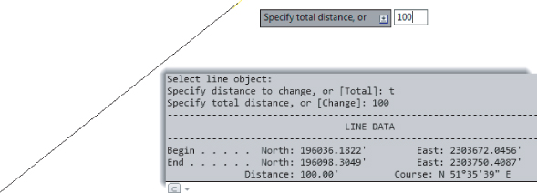
If instead you specify a total distance on the command line, the length of the line is changed to the distance you specify. The summary report shown in Figure 1.33 shows the same beginning coordinate as in Figure 1.32 but a different end coordinate, resulting in a total length of 100′ (30.5 m).
Figure 1.33 The summary report on a line where the command specified a total distance
Create Line From End Of Object Command
![]()
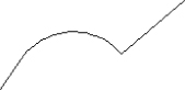
The Create Line From End Of Object command lets you draw a line tangent to the end of a line or arc of your choosing. Most commonly, you'll use this tool when re-creating deeds or other survey work where you have to specify a line that continues a tangent from an arc (see Figure 1.34).
Figure 1.34 The Create Line From End Of Object command lets you add a tangent line to the end of an arc.
Create Line Tangent From Point Command
![]()
![]()
The Create Line Tangent From Point command is similar to the Create Line From End Of Object command, but Create Line Tangent From Point allows you to choose a point of tangency that isn't the endpoint of the line or arc (see Figure 1.35).
Figure 1.35 The Create Line Tangent From Point command can place a line tangent at any point on an arc (or line).

Create Line Perpendicular From Point Command
![]()
Using the Create Line Perpendicular From Point command, you can specify that you'd like a line drawn perpendicular to any point of your choosing along a line or arc. In the example shown in Figure 1.36, a line is drawn perpendicular to the endpoint of the arc. This command can be useful when the distance from a known monument, perpendicular to a legally platted line, must be labeled in a drawing.
Figure 1.36 A perpendicular line is drawn from the endpoint of an arc, using the Create Line Perpendicular From Point command.
Re-creating a Deed Using Line Tools
The upcoming exercise will help you apply some of the tools you've learned so far to reconstruct the overall parcel.
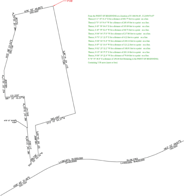
When you open up the file for the exercise, you will see a legal description with the following information (metric will have different lengths, of course):
From the POINT OF BEGINNING at a location of N 186156.65′,  E 2305474.07′
Thence, S 11° 45′ 41.4″ E for a distance of 693.77 feet to a point on a line.
Thence, S 73° 10′ 54.4″ W for a distance of 265.45 feet to a point on a line.
Thence, S 05° 59′ 04.4″ E for a distance of 185.89 feet to a point on a line.
Thence, S 45° 55′ 02.4″ W for a distance of 68.73 feet to a point on a line.
Thence, N 06° 04′ 37.0″ W for a distance of 217.80 feet to a point on a line.
Thence, N 73° 21′ 22.5″ E for a distance of 4.22 feet to a point on a line.
Thence, N 06° 04′ 51.6″ W for a distance of 200.14 feet to a point on a line.
Thence, S 87° 32′ 10.4″ W for a distance of 121.22 feet to a point on a line.
Thence, N 02° 25′ 32.2″ W for a distance of 168.91 feet to a point on a line.
Thence, N 15° 38′ 57.5″ E for a distance of 283.16 feet to a point on a line.
Thence, N 06° 19′ 22.4″ W for a distance of 79.64 feet to a point  on a line.
N 76° 55′ 49.8″ E a distance of 250.00 feet Returning to the POINT OF BEGINNING;
Containing 5.58 acres (more or less)
Follow these steps. (Note: The legal description for metric users is located in the DWG file as text.)
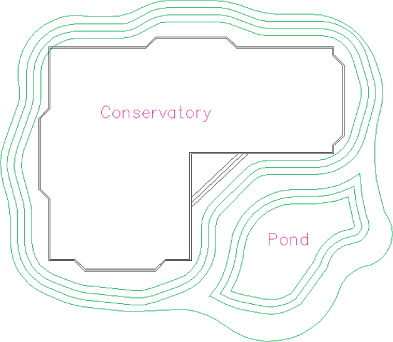
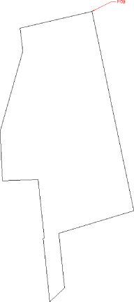
![]()
Figure 1.37 The finished linework
Creating Curves
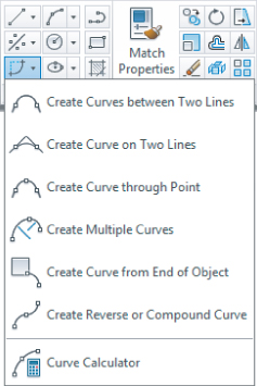
Curves are an important part of surveying and engineering geometry. The curves you create in this chapter are no different from AutoCAD arcs. What makes the curve commands unique from the basic AutoCAD commands isn't the resulting arc entity but the inputs used to draw the arc. Civil 3D wants you to provide directions to the arc commands using land surveying terminology rather than with generic Cartesian parameters. Figure 1.38 shows the Create Curves menu options.
Figure 1.38 Create Curves commands
Standard Curves
When re-creating legal descriptions for roads, easements, and properties, users such as engineers, surveyors, and mappers often encounter a variety of curves. Although standard AutoCAD arc commands could draw these arcs, the AutoCAD arc inputs are designed to be generic to all industries. The following curve commands have been designed to provide an interface that more closely matches land surveying, mapping, and engineering language.
Create Curve Between Two Lines Command
![]()
The Create Curve Between Two Lines command is much like the standard AutoCAD Fillet command, except that you aren't limited to a radius parameter. The command draws a curve that is tangent to two lines of your choosing. This command also trims or extends the original tangents so their endpoints coincide with the curve endpoints. The lines are trimmed or extended to the resulting PC (point of curve, which is the beginning of a curve) and PT (point of tangency, or the end of a curve). You may find this command most useful when you're creating foundation geometry for road alignments, parcel boundary curves, and similar situations.
The command prompts you to choose the first tangent and then the second tangent. The command line gives the following prompt:
Select entry [Tangent/External/Degree/Chord/Length/Mid-Ordinate/
miN-dist/Radius]<Radius>:
Pressing ![]() at this prompt lets you input your desired radius. As with standard AutoCAD commands, pressing T changes the input parameter to Tangent, pressing C changes the input parameter to Chord, and so on.
at this prompt lets you input your desired radius. As with standard AutoCAD commands, pressing T changes the input parameter to Tangent, pressing C changes the input parameter to Chord, and so on.
As with the Fillet command, your inputs must be geometrically possible. For example, your two lines must allow for a curve of your specifications to be drawn while remaining tangent to both. Figure 1.39 shows two lines with a 25′ (7.6 m) radius curve drawn between them. Note that the tangents have been trimmed so their endpoints coincide with the endpoints of the curve. If either line had been too short to meet the endpoint of the curve, that line would have been extended.
Figure 1.39 Two lines using the Create Curve Between Two Lines command
Create Curve On Two Lines Command
![]()
The Create Curve On Two Lines command is identical to the Create Curve Between Two Lines command, except that the Create Curve On Two Lines command leaves the chosen tangents intact. The lines aren't trimmed or extended to the resulting PC and PT of the curve.
Figure 1.40, for example, shows two lines with a 25′ (7.6 m) radius curve drawn on them. The tangents haven't been trimmed and instead remain exactly as they were drawn before the Create Curve On Two Lines command was executed.
Figure 1.40 The original lines stay the same after you execute the Create Curve On Two Lines command.
Create Curve Through Point Command
![]()
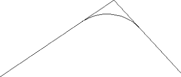
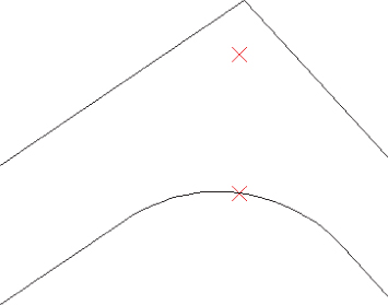
The Create Curve Through Point command lets you choose two tangents for your curve followed by a pass-through point. This tool is most useful when you don't know the radius, length, or other curve parameters but you have two tangents and a target location. It isn't necessary that the pass-through location be a true point object; it can be any location of your choosing.
This command also trims or extends the original tangents so their endpoints coincide with the curve endpoints. The lines are trimmed or extended to the resulting PC and PT of the curve.
Figure 1.41, for example, shows two lines and a desired pass-through point. Using the Create Curve Through Point command allows you to draw a curve that is tangent to both lines and that passes through the desired point. In this case, the tangents have been trimmed to the PC and PT of the curve.
Figure 1.41 The first image shows two lines with a desired pass-through point. In the second image, the Create Curve Through Point command draws a curve that is tangent to both lines and passes through the chosen point.
Create Multiple Curves Command
![]()
The Create Multiple Curves command lets you create several curves that are tangentially connected. The resulting curves have an effect similar to an alignment spiral section. This command can be useful when you are re-creating railway track geometry based on field- survey data.
The command prompts you for the two tangents. Then, the command line prompts you as follows:
Enter Number of Curves:
The command allows for up to 10 curves between tangents.
One of your curves must have a flexible length that's determined on the basis of the lengths, radii, and geometric constraints of the other curves. Curves are counted clockwise, so enter the number of your flexible curve:
Enter Floating Curve #:
Enter the length and radii for all your curves:
Enter curve 1 Radius:
Enter curve 1 Length:
The floating curve number will prompt you for a radius but not a length.
As with all other curve commands, the specified geometry must be possible. If the command can't find a solution on the basis of your length and radius inputs, it returns no solution (see Figure 1.42).
Figure 1.42 Two curves were specified with the #2 curve designated as the floating curve.
Create Curve From End Of Object Command
![]()
The Create Curve From End Of Object command enables you to draw a curve tangent to the end of your chosen line or arc.
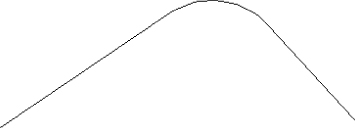
The command prompts you to choose an object to serve as the beginning of your curve. You can then specify a radius and an additional parameter (such as Delta or Length) for the curve or the endpoint of the resulting curve chord (see Figure 1.43).
Figure 1.43 A curve, with a 25′ (7.6 m) radius and a 30′ (9.1 m) length, drawn from the end of a line
Create Reverse Or Compound Curves Command
![]()
The Create Reverse Or Compound Curves command allows you to add additional curves to the end of an existing curve. Reverse curves are drawn in the opposite direction (i.e., a curve to the right tangent to a curve to the left) from the original curve to form an S shape. In contrast, compound curves are drawn in the same direction as the original curve (see Figure 1.44). This tool can be useful when you are re-creating a legal description of a road alignment that contains reverse and/or compound curves.
Figure 1.44 A tangent and curve before adding a reverse or compound curve (left); a compound curve drawn from the end of the original curve (right).
Best Fit Entities
Although engineers and surveyors do their best to make their work an exact science, sometimes tools like the Best Fit Entities are required.
Roads in many parts of the world have no defined alignment. They may have been old carriage roads or cart paths from hundreds of years ago that evolved into automobile roads. Surveyors and engineers are often called to help establish official alignments, vertical alignments, and right-of-way lines for such roads on the basis of a best fit of surveyed centerline data.
Other examples for using Best Fit Entities include property lines of agreement, road rehabilitation projects, and other cases where existing survey information must be approximated into “real” engineering geometry (see Figure 1.45).
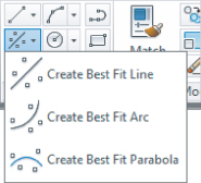
Figure 1.45 The Create Best Fit Entities menu options
Create Best Fit Line Command

The Create Best Fit Line command under the Best Fit drop-down on the Draw panel takes a series of Civil 3D points, AutoCAD points, entities, or drawing locations and draws a single best-fit line segment from this information. In Figure 1.46, for example, the Create Best Fit Line command draws a best-fit line through a series of points that aren't quite collinear. Note that the best-fit line will change as more points are picked.
Figure 1.46 A preview line drawn through points that aren't quite collinear

Once you've selected your points, a Panorama window appears with a regression data chart showing information about each point you chose, as shown in Figure 1.47.
Figure 1.47 The Panorama window lets you optimize your best fit.

This interface allows you to optimize your best fit by adding more points, excluding points, selecting the check box in the Pass Through column to force one of your points on the line, or adjusting the value under the Weight column.
Create Best Fit Arc Command

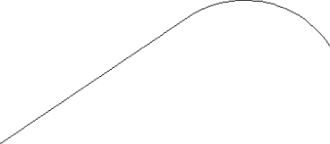
The Create Best Fit Arc command under the Best Fit drop-down works identically to the Create Best Fit Line command, except that the resulting entity is a single arc segment as opposed to a single line segment (see Figure 1.48)
Figure 1.48 A curve created by best fit

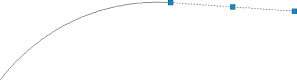
Create Best Fit Parabola Command
![]()
The Create Best Fit Parabola command under the Create Best Fit Entities option works in a similar way to the line and arc commands just described. This command is most useful when you have a triangulated irregular network (also known as TIN) sampled or surveyed road information, and you'd like to replicate true vertical curves for your design information.
After you select this command, the Parabola By Best Fit dialog appears (see Figure 1.49).
Figure 1.49 The Parabola By Best Fit dialog

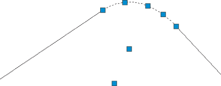
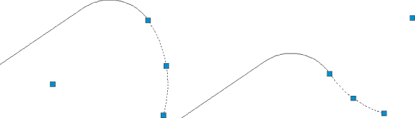
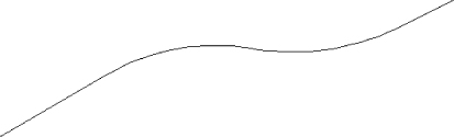
You can select inputs from entities (such as lines, arcs, polylines, or profile objects) or by clicking on screen. The command then draws a best-fit parabola on the basis of this information. In Figure 1.50, the shots were represented by AutoCAD points; more points were added by selecting the By Clicking On The Screen option and using the Node Osnap to pick each point.
Figure 1.50 The best-fit preview line changes as more points are picked.

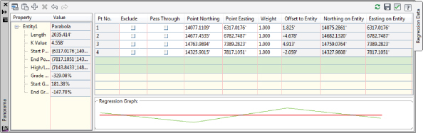
Once you've selected your points, a Panorama window (shown in Figure 1.51) appears, showing information about each point you chose. Also note the information in the right pane regarding K-value, curve length, grades, and so forth. You can optimize your K-value, length, and other values by adding more points, selecting the check box in the Pass Through column to force one of your points on the line, or adjusting the value under the Weight column.
Figure 1.51 The Panorama window lets you make adjustments to your best-fit parabola.
Attach Multiple Entities
![]()
The Attach Multiple Entities command (found on the Home tab in the Ribbon and extended Draw panel pull-down) is a combination of the Line From End Of Object command and the Curve From End Of Object command. This command is most useful for reconstructing deeds or road alignments from legal descriptions when each entity is tangent to the previous entity. Using this command saves you time because you don't have to constantly switch between the Line From End Of Object command and the Curve From End Of Object command (see Figure 1.52).
Figure 1.52 The Attach Multiple Entities command draws a series of lines and arcs so that each segment is tangent to the previous one

The Curve Calculator
![]()
Sometimes you may not have enough information to draw a curve properly. Although many of the curve-creation tools assist you in calculating the curve parameters, you may find an occasion where the deed you're working with is incomplete.
![]()
The Curve Calculator found in the Curves drop-down on the Draw panel helps you calculate a full collection of curve parameters on the basis of your known values and constraints. The units used in the Curve Calculator match the units assigned in your Drawing Settings.
The Curve Calculator can remain open on your screen while you're working through commands. You can send any value in the Calculator to the command line by clicking the button next to that value (see Figure 1.53).
Figure 1.53 The Curve Calculator

The button at the upper left of the Curve Calculator inherits the arc properties from an existing arc in the drawing, and the drop-down menu in the Degree Of Curve Definition selection field allows you to choose whether to calculate parameters for an arc or a chord definition.
The drop-down menu in the Fixed Property selection field also gives you the choice of fixing your Radius or Delta Angle when calculating the values for an arc or a chord, respectively (see Figure 1.54). The parameter chosen as the fixed value is held constant as additional parameters are calculated.
Figure 1.54 The Fixed Property drop-down menu gives you the choice of fixing your radius or delta value.

As explained previously, you can send any value in the Curve Calculator to the command line using the button next to that value. This ability is most useful while you're active in a curve command and would like to use a certain parameter value to complete the command.
Test your new line and curve knowledge, follow these steps. (You do not need to have completed the previous exercises to complete this one.)
Your completed lines and arcs will look like Figure 1.55, and they will be located just south of the property you entered in the previous exercise.
Figure 1.55 Lines and arcs of the completed exercise
Adding Line and Curve Labels
![]()
Although most robust labeling of site geometry is handled using Parcel or Alignment labels, limited line- and curve-annotation tools are available in Civil 3D. The line and curve labels are composed much the same way as other Civil 3D labels, with marked similarities to Parcel and Alignment Segment labels.
Our next exercise leads you through labeling the deed you entered earlier in this chapter:

Figure 1.56 The Add Labels dialog, with Label Type set to Multiple Segment

Figure 1.57 The labeled linework
Using Transparent Commands
You might be surprised to know that you have already been using a form of the transparent commands. If you used the Line By Point # Range command or the Line By Bearing command, you have already used a transparent command.
Transparent commands are “helper” commands that make base AutoCAD input more surveyor- and civil designer–friendly. Transparent commands can only be used when another command is in progress. They are “commands within commands” that allow you to choose your input based on what information you have.
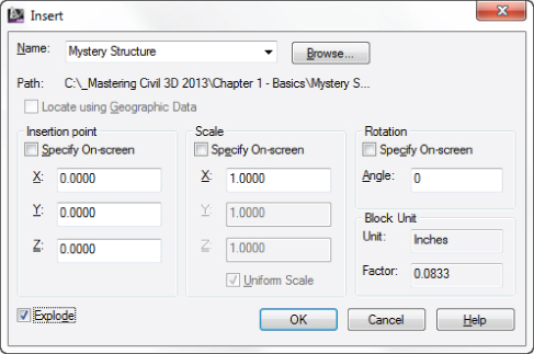
For example, you may have a plat whose information you are trying to input into AutoCAD. You may need to insert a block at a specific Northing and Easting. While the line command has a built-in option for Northing Easting, the insert command does not, and a transparent command will help you. In this case, you would start the Insert command with the Specify On Screen option checked. Before you click to place the block in the graphic, click the Northing Easting transparent command. The command line will then walk you through placing the block at your desired location.
While a transparent command is active, you can press Esc once to leave the transparent mode but stay active in your current command. You can then choose another transparent command if you'd like. For example, you can start a line using the Endpoint Osnap, activate the Angle Distance transparent command, draw a line-by-angle distance, and then press Esc, which takes you out of angle-distance mode but keeps you in the line command. You can then draw a few more segments using the Point Object transparent command, press Esc, and finish your line with a Perpendicular Osnap.
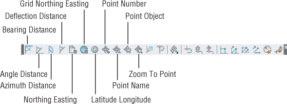
You can activate the transparent commands using keyboard shortcuts or using the Transparent Commands toolbar. Be sure you include the Transparent Commands toolbar (shown in Figure 1.58) in all your Civil 3D and survey-oriented workspaces.
Figure 1.58 The Transparent Commands toolbar
The six profile-related transparent commands will be covered in Chapter 7, “Profiles and Profile Views.”
Standard Transparent Commands
![]()
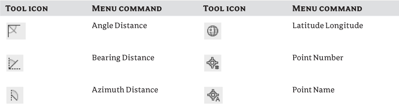
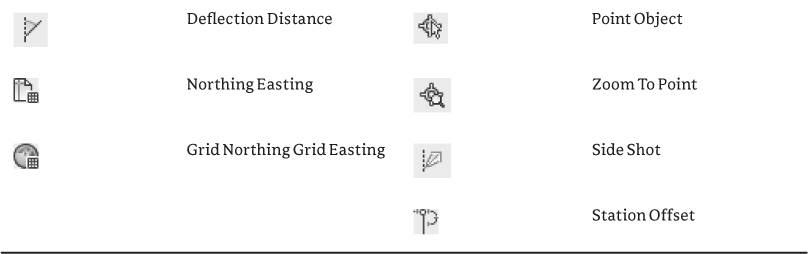
The transparent commands shown in Table 1.2 behave identically to their like-named counterparts from the Draw panel (discussed earlier in this chapter). The difference is that you can call up these transparent commands in any appropriate AutoCAD or Civil 3D draw command, such as a line, polyline, alignment, parcel segment, feature line, or pipe-creation command.
Table 1.2 The transparent commands used in plan view
Matching Transparent Commands
You may have construction or other geometry in your drawing that you'd like to match with new lines, arcs, circles, alignments, parcel segments, or other entities.
![]()
While actively drawing an object that has a radius parameter, such as a circle, an arc, an alignment curve, or a similar object, you can choose the Match Radius transparent command and then select an object in your drawing that has your desired radius. Civil 3D draws the resulting entity with a radius identical to that of the object you chose during the command. You'll save time using this tool because you don't have to first list the radius of the original object and then manually type in that radius when prompted by your circle, arc, or alignment tool.
![]()
The Match Length transparent command works identically to the Match Radius transparent command except that it matches the length parameter of your chosen object.
Some people find working with transparent commands awkward at first. It feels strange to move your mouse away from the drawing area and click an icon while another command is in progress. Try a few transparent commands to get the feel for how they operate:
![]()
![]()
Figure 1.59 Using the Insert command to place a block
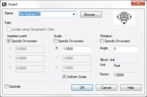
![]()
You should now see the fire hydrant symbol at the specified station, on the left of the alignment.
The Bottom Line
Find any Civil 3D object with just a few clicks.
By using Prospector to view object data collections, you can minimize the panning and zooming that are part of working in a CAD program. When common subdivisions can have hundreds of parcels or a complex corridor can have dozens of alignments, jumping to the desired one nearly instantly shaves time off everyday tasks.
Master It
Open BasicSite.dwg from www.sybex.com/go/masteringcivil3d2013, and find parcel number 18 without using any AutoCAD commands or scrolling around on the drawing screen. (Hint: Take a look at Figure 1.5.)
Modify the drawing scale and default object layers.
Civil 3D understands that the end goal of most drawings is to create hard-copy construction documents. By setting a drawing scale and then setting many sizes in terms of plotted inches or millimeters, Civil 3D removes much of the mental gymnastics that other programs require when you're sizing text and symbols. By setting object layers at a drawing scale, Civil 3D makes uniformity of drawing files easier than ever to accomplish.
Master It
Change the Annotation scale in the model tab of BasicSite.dwg from the 100-scale drawing to a 40-scale drawing. (For metric users: Use BasicSite_METRIC.dwg and change the scale from 1:1000 to 1:500.)
Navigate the Ribbon's contextual tabs.
As with AutoCAD, the Ribbon is the primary interface for accessing Civil 3D commands and features. When you select an AutoCAD Civil 3D object, the Ribbon displays commands and features related to that object. If several object types are selected, the Multiple contextual tab is displayed.
Master It
Continue working in the file BasicSite.dwg (Basic Site_METRIC.dwg). It is not necessary to have completed the previous exercise to continue. Using the Ribbon interface, access the Alignment properties for Road A.
Create a curve tangent to the end of a line.
It's rare that a property stands alone. Often, you must create adjacent properties, easements, or alignments from their legal descriptions.
Master It
Open the drawing MasterIt.dwg (MasterIt_METRIC.dwg). Create a curve tangent to the east end of the line labeled in the drawing. The curve should meet the following specifications:
- Radius: 200.00′ (60 m)
- Arc Length: 66.580′ (20 m)
Label lines and curves.
Although converting linework to parcels or alignments offers you the most robust labeling and analysis options, basic line- and curve-labeling tools are available when conversion isn't appropriate.
Master It
Add line and curve labels to each entity created in MasterIt.dwg or MasterIt_Metric.dwg. It is recommended you complete the previous exercise so you will have a curve to work with. Choose a label that specifies the bearing and distance for your lines and length, radius, and delta of your curve.