Chapter 11

Advanced Corridors, Intersections, and Roundabouts

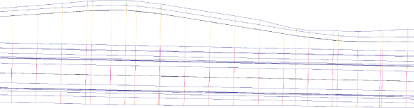
In Chapter 10, “Basic Corridors,” you built several simple corridors — including an example where the road lane used an alignment and profile target to add a variable width and elevation to the edge of traveled way — and began to see the dynamic power of the corridor model. The focus of that chapter was to get things started, but it's unrealistic to think that a project would have only one road in the middle of nowhere with no intersections, no adjustments, and no complications. You may be having trouble visualizing how you'll build a corridor to tackle your more complex design projects, such as the one pictured in Figure 11.1.

Figure 11.1 A corridor model for the example subdivision

This chapter focuses on taking your corridor-modeling skills to a new level by introducing more tools to your corridor-building toolbox, such as intersecting roads, cul-de-sacs, advanced techniques, and troubleshooting. It deals with a roadside swale that follows a variable horizontal alignment, as well as a vertical profile that doesn't follow the centerline of the road. This happens frequently when existing culvert crossings must be met, or when you have different slope requirements for the roadside swale.

This chapter assumes that you've worked through the examples in the alignments, profiles, profile view, assemblies, and basic corridor chapters. Without a strong knowledge of the foundation skills, many of the tasks in this chapter will be difficult.

In this chapter, you will learn to:

• Create corridors with noncenterline baselines
• Add alignment and profile targets to a region for a cul-de-sac
• Create a surface from a corridor and add a boundary

Corridor Utilities

To create an alignment and profile for the swale, you'll take advantage of some of the corridor utilities found in the Launch Pad panel (Figure 11.2) by selecting the corridor.

Figure 11.2 A bounty of corridor utilities on the Launch Pad panel

The utilities on this panel are as follows:

Using Alignment and Profile Targets to Model a Roadside Swale

The following exercise takes you through revising a model from a symmetrical corridor with roadside swales to a corridor with a transitioning roadside swale centerline. You'll also take advantage of some of the static extraction corridor utilities discussed in the previous section:

1. Open the Corridor Swale.dwg (Corridor Swale_METRIC.dwg) file, which you can download from this book's web page at www.sybex.com/go/masteringcivil3d2013.

Note that the drawing contains a symmetrical corridor (see Figure 11.3), which was built using an assembly that includes two roadside swales. This drawing has been split into two modelspace views so you can see what is going on in plan and in profile at the same time.

Figure 11.3 The initial corridor with symmetrical roadside swales

2. Select the corridor, and choose the Alignment From Corridor tool from the Launch Pad panel.

3. When prompted, pick the corridor feature line that represents the swale on the left side of the road centerline, as noted in the drawing, to create an alignment.

Note that if you select one of the corridor feature lines to activate the Corridors tab, that feature line will be created by default. You can pick one of the frequency lines to avoid this potential pitfall!

4. In the Create Alignment From Objects dialog (Figure 11.4),

a. Name the alignment Swale Left.

b. Keep the default value for Site And Style.

c. Change the Alignment Label Set to All Labels, as shown in Figure 11.4.

Figure 11.4 The Create Alignment From Objects dialog appears when you're extracting a feature line to an alignment.

5. Be sure to uncheck Create Profile, and then click OK to finish.

6. Press Esc to exit the command.

You should now have a new alignment with labels in the plan view, as shown in Figure 11.5.

Figure 11.5 The extracted alignment

Next, you will extract the profile in a separate step. By performing these actions in two steps, you ensure that the profile will be associated with the main alignment, rather than with the offset alignment you created in the previous step. Keeping the extracted profile with the main alignment will allow you to work on the profile in the same profile view as the proposed centerline.

7. Select the corridor by clicking a frequency line or feature line and select Profile From Corridor from the drop-down list on the Launch Pad panel of the contextual Ribbon tab.

8. Select the same Swale Left feature line as you did in the previous step.

You may need to use the DRAWORDER command or press Ctrl+W on your keyboard to access the feature line hiding behind the new alignment. When the feature line is selected, you will see the Create Profile dialog, as shown in Figure 11.6.

Figure 11.6 Create Profile dialog

9. Name the profile Swale Left Profile and click OK.

You should now see the profile you just created in the bottom viewport. The profile represents the vertical path of the feature line representing the swale centerline, as shown in Figure 11.7.

Figure 11.7 A portion of the resulting extracted profile

10. Select your newly extracted Left Swale Profile. From the Profile contextual tab ⇒ Modify Profile panel, select Geometry Editor.

11. From the Profile Layout Tools Toolbar, click Move PVI.

12. Zoom in to station 46+00 (1+400 for metric users) if necessary, and select the PVI at 1182.93′ (360.72 m) in elevation to elevation 1170′ (356.50 m), as shown in Figure 11.8. Press Esc to exit the command.

Figure 11.8 Move a PVI to provide an exaggerated low spot.

13. Select the corridor and from the Corridor Contextual tab ⇒ Modify Panel, select Corridor Properties. Switch to the Parameters tab.

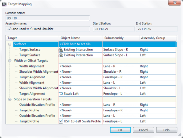
14. There is just one baseline and region in this project. Scroll over to the ellipsis button to open the Target Mapping dialog on the same line as the region.

When setting a surface target for a corridor, going to Set All Targets will work great. As your corridors get more complex, the number of options for elevation and offset targets become more numerous. By getting in the habit of targeting objects at the region level, you'll save yourself a lot of looking.

15. In the Width or Offset Target area (Figure 11.9), set the Foreslope - L subassembly to target the Swale Left Target Alignment.

Figure 11.9 Set the Foreslope - L subassembly to follow the Swale Left alignment and profile.

16. In the Slope or Elevation Targets area, set the Foreslope - L subassembly to target the Swale Left Profile.

Figure 11.9 shows the Target Mapping dialog with the alignments and profiles appropriately mapped.

17. Click OK to dismiss the Target Mapping dialog, and click OK again to dismiss the Corridor Properties dialog and rebuild the corridor.

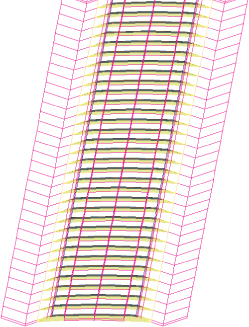
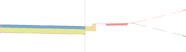
The subtle change you made in the corridor can be observed at station 46+00 (or 1+400 for metric users), as shown in Figure 11.10.

Figure 11.10 The adjusted corridor

Note that the corridor has been adjusted to reflect the new target alignment and profile. Also note that you may want to increase the sampling frequency. You can view the sections using the View/Edit Corridor Section tools. You can also view the corridor in 3D by picking it, right-clicking, and choosing Object Viewer. Use the 3D Orbit tools to change your view of the corridor.

Multiregion Baselines

A question many people ask when working with corridors is, “At what point do I need another region?” The answer is simple: If you need a different assembly, you need a different region.

In the following example, you will step through adding an additional region to an existing baseline:

1. Open the drawing Multi-RegionCorridor.dwg (Multi-RegionCorridor_METRIC.dwg).

This drawing has been split into two modelspace viewports so that you can observe the results of your efforts in 3D.

2. Select the corridor and, from the Corridor contextual tab ⇒ Modify Corridor panel, select Corridor Properties.

On the Parameters tab, notice there is a baseline containing a single region.

3. Right-click on the region and select Split Region, as shown in Figure 11.11.

Figure 11.11 Right-click to access region creation tools.

4. At the command line, enter 4000 (1220 for metric users) to create a split at 40+00 (1+220 for metric users), and create a second split at 55+00 (1+680 for metric users) by entering 5500 (1680 ).

5. Press again to return to the Corridor Parameters dialog.

If you see a warning dialog referring to 0+00 being outside of the station limits, click OK and continue.

You should have three regions at this step, as shown in Figure 11.12.

Figure 11.12 New regions with different assemblies applied

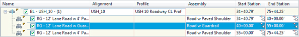
6. Change the assembly for the middle region to use the Road w Guardrail assembly, and then click OK.

7. Scroll over and click the Target ellipsis button.

8. Verify that the targets have been maintained for this region. If necessary, set the targets as shown in Figure 11.13.

Figure 11.13 Targets for the middle region

9. Click OK when Target Mapping is complete, and then click OK.

10. Select Rebuild when prompted.

You should now see additional feature lines in the plan view representing the top of the guardrail. In the right viewport, it will resemble Figure 11.14.

Figure 11.14 The completed corridor with guardrails

Modeling a Cul-de-Sac

Even if you never plan to design one in real life, understanding what is going on in a cul-de-sac corridor model will set you on the right path for building more complex models. If you truly understand the principles explained in the section that follows, then expanding your repertoire to include intersections and roundabouts will become much easier.

Using Multiple Baselines

Up to this point, every corridor we've examined has had a single baseline. In our examples, the centerline alignment has been the main driving force behind the corridor design. In this section, the training wheels are coming off! You've seen the last of single baseline corridors in this book.

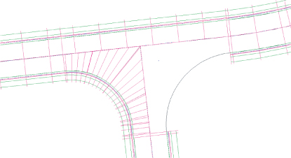
A cul-de-sac by itself can be modeled in two baselines, as shown in Figure 11.15. The procedures that follow will work for most cul-de-sacs, symmetrical, asymmetrical, and hammerhead styles. You will need the centerline alignment and design profile, as well as an edge of pavement alignment and design profile.

Figure 11.15 Example cul-de-sac alignment setup

In the section leading to the cul-de-sac bulb, the corridor can be modeled using the tools you learned in Chapter 10. In the example shown in Figure 11.15, the centerline of the road is the baseline, with an assembly using two lanes and with the crown as the baseline marker from beginning station to 1+47 (for metric users 0+045). However, once the curvature of the bulb starts at 1+47.00 (for metric users 0+045), the centerline is no longer an acceptable baseline.

Assemblies are always applied to a baseline and the geometry will be perpendicular to the baseline. To get correct pavement grades in the bulb, you'll need to hop over to the edge of pavement alignment for a baseline. This second baseline will use a partial assembly that is built with the main assembly marker at the outside edge of pavement (Figure 11.16). The crown of the road will stretch to meet the centerline alignment and profile as its targets.

Figure 11.16 Assembly used for designing off the edge of pavement

It helps to think of the assembly as radiating away from the baseline, from the assembly base outward, toward a target (Figure 11.17). Because the assemblies are applied to the baseline in a perpendicular manner, using the edge of pavement for a baseline in curved areas (such as cul-de-sac bulbs or curb returns) will result in a smooth, properly graded pavement surface.

Figure 11.17 It helps to think of the assemblies radiating away from the baseline toward the targets.

Establishing EOP Design Profiles

One of the most challenging parts of any “fancy” corridor (i.e., cul-de-sac, intersection, or roundabout) is establishing design profiles for noncenterline alignments. You must have design profiles for every alignment used as a target — there's no way around it — but it does not have to be a painful process to obtain them.

Using a simple, preliminary corridor and the profile creation tools you learned in Chapter 7, “Profiles and Profile Views,” you'll find that establishing an edge of pavement (EOP) profile can go quickly.

In the exercise that follows, you will work through the steps of creating an EOP profile:

1. Open the Cul-de-sac_Profile.dwg (Cul-de-Sac_Profile_METRIC.dwg)file, which you can download from this book's web page.

This drawing contains several alignments and an existing surface whose style is set to show the border only.

2. From the Home tab ⇒ Create Design Panel, click Corridor, and do the following:

A. Name the corridor PRELIM.

B. Set Alignment to Frontenac Drive.

C. Set Profile to Frontenac Drive - FG.

D. Set Assembly to PRELIM

E. Clear the checkbox for Set Baseline And Region Parameters.

3. No targets are needed in this preliminary corridor, so click OK to complete the corridor.

4. Select the new corridor and open the Corridor Properties.

5. On the Surfaces tab, click the leftmost button to start a corridor surface.

6. With Data Type set to Links and Code set to Top, click the plus sign to add data to the surface.

7. On the Boundaries tab, right-click the PRELIM Surface, and select Corridor Extents as Outer Boundary.

8. Click OK and rebuild the corridor.

You should now see contours in your drawing representing the 2 percent crossfall from the centerline.

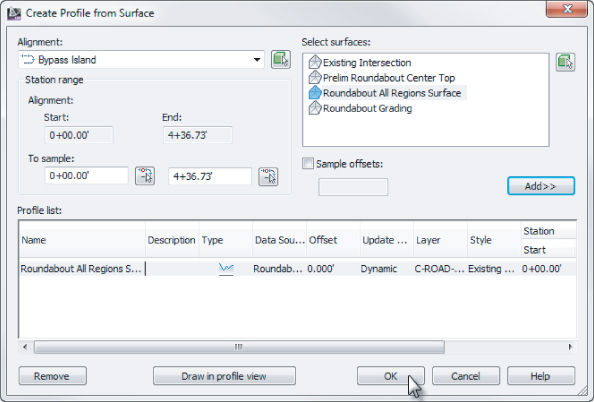
9. Select the red EOP alignment for the cul-de-sac, and in the contextual Ribbon tab, click Surface Profile.

10. In the Create Profile From Surface dialog, highlight PRELIM Surface - (1) and click Add.

11. Click the Draw In Profile View button.

12. Leave all the defaults in the Create Profile View dialog and click Create Profile View.

13. Click in the graphic to the right of the surface to place the profile view.

The profile you are seeing will have gaps in the middle that need grading information. However, the bulb portion of the profile only needs to exist between 16+87.00 (0+514.2 for metric users) and 19+42.89 (0+592.2 for metric users). They are the PC and PT stations for the EOP alignment in plan. In this example, you will create a design profile that starts slightly before, and ends slightly after, these critical stations.

14. Select the profile view and click Profile Creation Tools on the contextual Ribbon tab.

15. Click OK to accept the defaults in the Create Profile dialog.

16. In the Profile Layout toolbar, select Draw Tangents, and snap to the intersection of the preliminary profile and the grid line at 16+50 (0+500 for metric users). The elevation is also determined by this location.

17. Next, snap to the endpoint where the preliminary surface trails off at station 17+02.38 (0+517.13 for metric users) elevation 792.88′ (241.737 m).

18. The next VPI will be the peak of the preliminary profile in the center of the view; station 18+14.94 (0+553.20 for metric users), elevation 790.35′ (240.898 m).

19. Snap to the endpoint where the preliminary profile picks up again; station 19+27.51 (0+589.26 for metric users), elevation 792.88′ (241.737 m).

20. Finally, snap to the grade break at station 19+78.30 (0+605.99 for metric users), elevation 794.68′ (242.351 m).

21. Press to complete the command and close the Profile Layout tools.

You now have a proposed profile that is acceptable to use in the cul-de-sac corridor.

Putting the Pieces Together

You have all the pieces in place to perform the first iterations of this cul-de-sac design.

The following exercise will walk you through the steps to put the cul-de-sac together. You will complete several steps and let the corridor build to observe what is happening at each stage. This exercise will also encourage you to get comfortable using Corridor Properties to make design modifications.

1. Open the Cul-de-sac_Design.dwg (Cul-de-Sac_Design_METRIC.dwg) file, which you can download from this book's web page.

This drawing contains the cul-de-sac centerline alignment and profile, the EOP alignment and profile, and the assemblies needed to complete the process. The PRELIM corridor layer is frozen. The view of this drawing is twisted 90ινϕτψ to better fit most monitors.

2. From the Home tab, on the Create Design panel select Corridor, and do the following:

a. Name the corridor Cul-de-Sac.

b. Set Alignment to Frontenac Drive.

c. Set Profile to Frontenac Drive FG.

d. Set Assembly to Urban.

e. Set Target Surface to EG.

f. Keep the checkmark next to Set Baseline And Region Parameters.

g. Click OK.

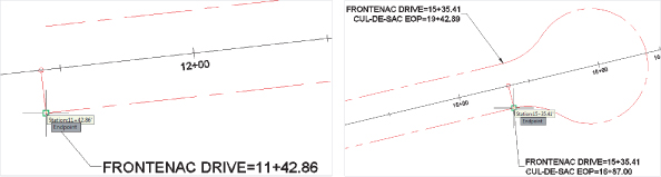
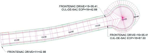
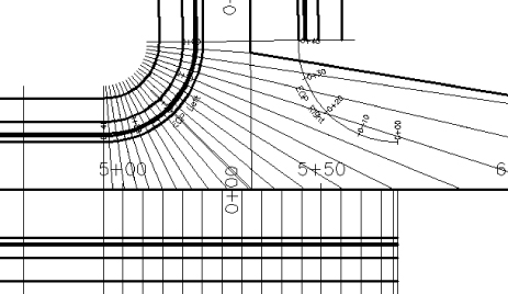
3. In the Baseline And Region Parameters dialog, click the Pick Station button for the start station of the first region.

4. Snap to the start of the EOP alignment on the west side, as shown in Figure 11.18 (left).

Figure 11.18 Setting the start station (left) and end station (right) for the centerline region

This will result in a start station of 11+42.86 (0+348.34 for metric users) in the Create Corridor dialog.

5. Click the Pick Station icon for the end station of the first region.

6. Snap to the PT station on the east side of the cul-de-sac bulb, as shown in Figure 11.18 (right).

This will result in the region end station of 15+35.41 (0+467.99 for metric users).

7. Click OK to dismiss the Baseline And Region Parameters dialog, and click OK to complete the initial piece of the corridor.

Examine the corridor you just created. It should start south of the intersection with the Syrah Way alignment, and end before the curvy part of the cul-de-sac bulb.

8. Select the corridor and click Corridor Properties.

If necessary, correct any station problems with the first region.

9. In the Parameters tab of Corridor Properties, click Add Baseline.

10. Select the Cul-de-Sac EOP as the alignment, and click OK.

11. In the Profile Column, click <Click here…>, and select the Cul-de-Sac EOP - FG profile.

This is the profile that you learned how to develop in the previous exercise.

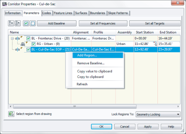
12. Right-click on the newly added baseline, and select Add Region, as shown in Figure 11.19.

Figure 11.19 Right-click the baseline to add a region.

13. Select the Curb Right assembly, and click OK.

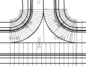
14. Expand the Cul-de-Sac baseline and then click the Pick Station button for the Curb Right region start station.

15. Select the PC station of the corridor bulb.

This will result in a start station value of 16+87.00 (0+514.20 for metric users).

16. Click the Pick Station icon for the end station of the region.

17. Select the PT station of the corridor bulb.

This will result in an end station of 19+42.89 (0+592.19 for metric users).

18. Click OK and let the corridor build once again.

Have a look at the corridor in its current state (see Figure 11.20). Even if you are not exactly sure what you are looking at, you should at least see a few things are amiss with the corridor so far.

Figure 11.20 The cul-de-sac corridor several steps away from completion

There are three things that need to be modified before the cul-de-sac is complete. The lane needs to extend to the center of the cul-de-sac bulb and the daylight surface needs to be set, both of which can be corrected in the Target Mapping area. Finally, you will want to increase the frequency around the curvy area to get a smoother, more precise design.

In the next steps, you will correct these issues and complete the cul-de-sac.

19. Select the corridor and return to Corridor Properties (last time in this exercise, we promise).

20. Scroll over and click the ellipsis to enter the Target Mapping dialog for the region named RG - Curb Right - (36).

The number following the region name may vary.

a. Set Target Surface to EG, and then click OK.

b. Set Width Alignment for Lane - L to Frontenac Drive. Click Add and then click OK.

c. Set Outside Elevation Profile to Frontenac Drive-FG for Lane - L. Click Add and then click OK.

d. Click OK again to dismiss the Target Mapping dialog.

21. Click the frequency ellipsis next to the current value of 25′ (20 m), and set the frequency for both tangents and curves to 5′ (1 m). Set the At Offset Target Geometry Points to Yes.

22. Click OK to dismiss the Frequency dialog.

23. Click OK and let the corridor rebuild one last time.

The completed corridor will look like Figure 11.21.

Figure 11.21 The completed cul-de-sac corridor. Gorgeous!

Troubleshooting Your Cul-de-Sac

People make several common mistakes when modeling their first few cul-de-sacs:

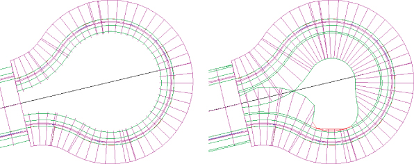
Your cul-de-sac appears with a large gap in the center.

If your curb line seems to be modeling correctly but your lanes are leaving a large empty area in the middle (see Figure 11.22), chances are pretty good that you forgot to assign targets or perhaps assigned the incorrect targets.

Figure 11.22 A cul-de-sac without targets

Fix this problem by opening the Target Mapping dialog for your region and checking to make sure you assigned the road centerline alignment and FG profile for your transition lane. If you have a more-advanced lane subassembly, you may have accidentally set the targets for another subassembly somewhere in your corridor instead of the lane for the cul-de-sac transition, especially if you have poor subassembly-naming conventions. Poor naming conventions become especially confusing if you used the Map All Targets button.

Your cul-de-sac appears to be backward.

Occasionally, you may find that your lanes wind up on the wrong side of the EOP alignment, as shown in Figure 11.23. The direction of your alignment will dictate whether the lane will be on the left or right side. In the example from the previous exercise, the alignment was running counterclockwise around the cul-de-sac bulb; therefore, the lane was on the left side of the assembly.

Figure 11.23 A cul-de-sac with the lanes modeled on the wrong side without targets (left) and with targets (right)

You can fix this problem by changing the assembly to the correct side.

Your cul-de-sac drops down to 0.

A common problem when you first begin modeling cul-de-sacs, intersections, and other corridor components is that one end of your baseline drops down to 0. You probably won't notice the problem in plan view, but once you build your surface (see Figure 11.24, left) or rotate your corridor in 3D (see Figure 11.24, right), you'll see it. This problem will always occur if your region station range extends beyond the proposed profile.

Figure 11.24 Contours indicating that the corridor surface drops down to 0 (right), and a corridor viewed in 3D showing a drop down to 0 (left)

The fix for this is the same as what you saw in the first exercise in Chapter 10 — that is, make sure your region station range corresponds with the design profile length. You may need to extend the design profile in some cases, but usually the station range will do the trick.

Your cul-de-sac seems flat.

When you're first learning the concept of targets, it's easy to mix up baseline alignments and target alignments. In the beginning, you may accidentally choose your EOP alignment as a target instead of the road centerline. If this happens, your cul-de-sac will look similar to Figure 11.25.

Figure 11.25 A flat cul-de-sac with the wrong lane target set

You can fix this problem by opening the Target Mapping dialog for this region and making sure the target alignment is set to the road centerline and the target profile is set to the road centerline FG profile.

Intersections: The Next Step Up

Ask yourself the following question: “Did I understand why we did what we did to build the cul-de-sac in the previous section?” If the answer is “Not really,” you may want to review a few topics before proceeding. If the answer is, “Yeah, mostly,” then you are ready to move to the next level of corridor complexity: intersections.

The steps that follow apply to all intersections, regardless of whether it is a T-shaped intersection, a four-way intersection, perfectly perpendicular, or skewed at an angle.

Corridor modeling is an iterative process. The more advanced your model, the more iterations it may take to get to the correct design. You will often not know the final design parameters until you see how the model relates to existing conditions or ties into other pieces of the design. Get comfortable jumping in and out of corridor properties and identifying regions within your corridor.

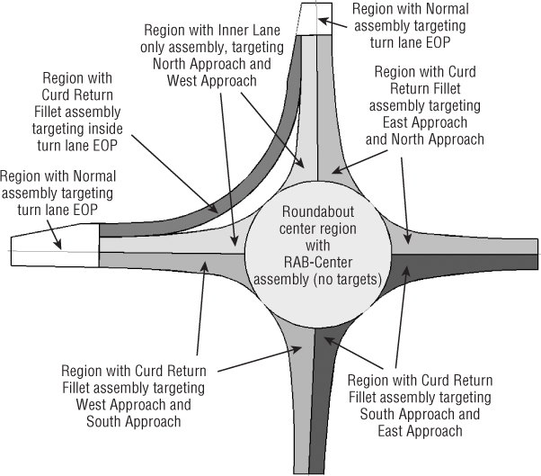
Plan what alignments, profiles, and assemblies you'll need to create the right combination of baselines, regions, and targets to model an intersection that will interact the way you want. It helps to create a simple sketch, as shown in Figure 11.26.

Figure 11.26 Plan your intersection model in sketch form.

Figure 11.27 shows a sketch of required baselines. As you saw in the previous example, baselines are the horizontal and vertical foundation of a corridor. Each baseline consists of an alignment, and its corresponding finished ground (FG) profile. You may never have thought of edge of pavement (EOP) in terms of profiles, but after you build a few intersections, thinking that way will become second nature. The Intersection tool on the Create Design panel of the Home tab will create EOP baselines as curb return alignments for you, but it will rely on your input for curb return radii.

Figure 11.27 Required baselines for modeling a typical intersection

Figure 11.28 breaks each baseline into regions where a different assembly or different target will be applied. Once the intersection has been created, target mapping as well as other particulars can be modified as needed.

Figure 11.28 Required regions for modeling an intersection created by the Intersection tool

Using the Intersection Wizard

All the work of setting baselines, creating regions, setting targets, and applying the correct frequencies can be done manually for an intersection. However, Civil 3D contains an automated Intersection tool that can handle many types of intersections.

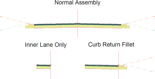
On the basis of the schematic you drew of your intersection, your main road will need several assemblies to reflect the different road cross sections. Figure 11.29 shows the full range of potential assemblies you may need in an intersection and the design situations in which they may arise.

Figure 11.29 Various assembly schematics and applications

Assembly Sets

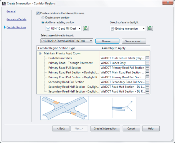
When you are ready to create an intersection, you do not need to have all the special assemblies created ahead of time. On the Corridor Regions page of the Create Intersection wizard, you will see a list of the assemblies Civil 3D plans to use. If the assemblies are not already part of the drawing, they will get pulled in automatically when you click Create Intersection.

The default intersection assemblies are general, and may not work for your design situation. You will want to create and save an assembly set of your own.

1. In a file that contains all of your desired assemblies, work through the Create Intersection wizard to get to the Corridor Regions page.

2. Click the ellipsis to select the appropriate assembly for each Corridor Region Section Type.

3. Once the listing is complete, click the Save As A Set button.

Civil 3D creates an XML file that stores the listing of the assemblies. It also creates a copy of each assembly as a separate DWG file. Save the set in a network shared location so your office colleagues can use the set as well.

The next time an intersection is created, you can use the assembly set by clicking Browse and selecting the XML file. Civil 3D will pull in your assemblies, saving lots of time!

This exercise will take you through building a typical peer-road intersection using the Create Intersection wizard:

1. Open the Intersection.dwg (Intersection_METRIC.dwg) file, which you can download from this book's web page.

The drawing contains two centerline alignments (USH 10 and Mill Creek Drive) that are part of the same corridor.

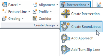
2. From the Home tab ⇒ Create Design panel, choose the Intersections ⇒ Create Intersection tool.

3. Using the Intersection object snap, choose the intersection of the two existing alignments.

4. When prompted to select the main road alignment, click the USH 10 alignment that runs vertically in the project.

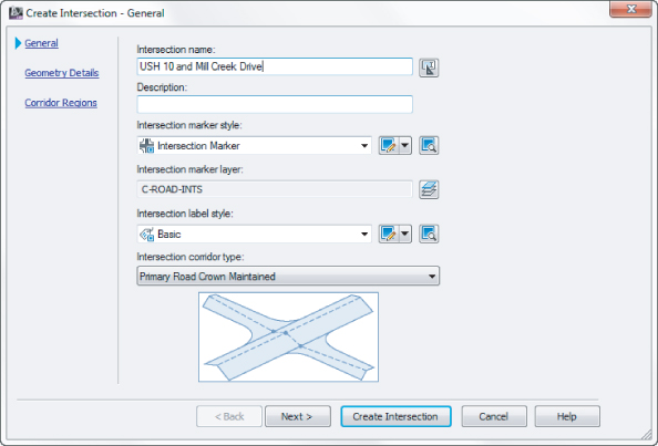
The Create Intersection – General dialog will appear (Figure 11.30).

Figure 11.30 The Create Intersection – General dialog

5. Name the intersection USH 10 and Mill Creek Drive. Set the Intersection corridor type to Primary Road Crown Maintained, as shown in Figure 11.30, and click Next.

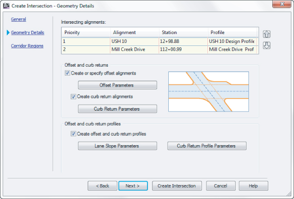
6. In the Geometry Details page (Figure 11.31), verify that USH 10 is the primary road by looking at the Priority listing. If USH 10 is not at the top of the list, use the arrow buttons on the right side to reorder the roads.

Figure 11.31 The Geometry Details page of the Create Intersection wizard

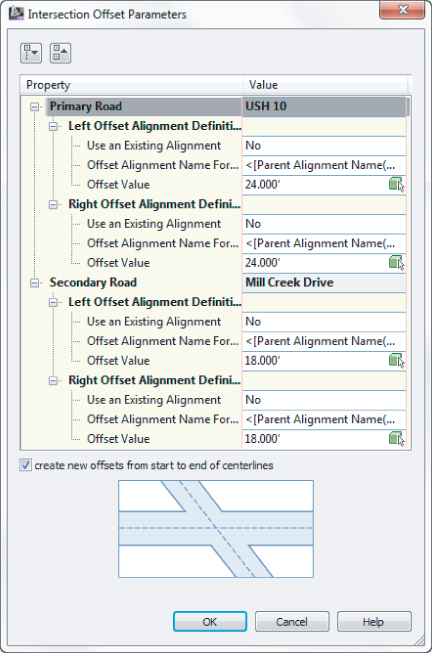
7. Click the Offset Parameters button, and do the following:

A. Set the offset values for both the left and right sides to 24′ (8 m) for USH 10.

B. Set the left and right offset values for Mill Creek Drive to 18′ (5 m).

C. Select the check box Create New Offsets From Start To End Of Centerlines.

At this step, the screen should resemble Figure 11.32.

Figure 11.32 Intersection Offset Parameters dialog

D. Click OK to close the Intersection Offset Parameters dialog.

8. Click the Curb Return Parameters to enter the Curb Return Parameters dialog.

A. For all four quadrants of the intersection, place a check mark next to Widen Turn Lane For Incoming Road and Widen Turn Lane For Outgoing Road.

B. Click the Next button at the top of the dialog to move from quadrant to quadrant.

As shown in Figure 11.33, a temporary glyph will help you determine which quadrant you are currently modifying.

Figure 11.33 Adding lane widening to the SW – Quadrant of the intersection

When you reach the last quadrant, you will see that the Next button is grayed out. This means that you have successfully worked through all four curb returns.

C. Click OK to return to wizard's Geometry Details page.

Some locales require that lane slopes flatten out to a 1% cross-slope in an intersection. If this is the case for you, you can change the lane slope parameters in the Intersection Lane Slope Parameters dialog (Figure 11.34). In this exercise you will leave this as 2%.

Figure 11.34 Lane slope parameters control the cross-slope in the intersection.

Civil 3D is performing the task of generating the curb return profile. The profile will be at least as long as the rounded curb plus the turn lanes that are added in this exercise. If you wish to have Civil 3D generate even more than the length needed, you can specify that in the Intersection Curb Return Profile Parameters area (Figure 11.35).

Figure 11.35 Intersection Curb Return Profile Parameters options extend the Civil 3D-generated profile beyond the curb returns by the value specified.

You will be keeping all default settings in both the Lane Slope Parameters area (Figure 11.34) and the Curb Return Parameters area (Figure 11.35).

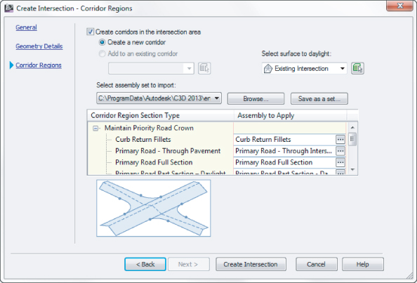
9. Click Next to continue to the Corridor Regions page (Figure 11.36).

Figure 11.36 The Corridor Regions page drives the assemblies used in the intersection.

The Corridor Regions page is where you control which assemblies are used for the different design locations around the intersection. Clicking each entry in the Corridor Region Section Type list will give you a clear picture of which assemblies you should use and where (as shown at the bottom of Figure 11.36). If your assemblies have the same names as the default assemblies, as is the case in this example, they will be pulled from the current drawing. Alternately, you can click the ellipsis to select any assembly from the drawing.

If you don't have all the necessary assemblies at this point, you can still create your intersection. Civil 3D will pull in the default set of assemblies. You can always modify these assemblies after they are brought in.

10. Click through the Corridor Region Section Type list to view the schematic preview for each.

Do not make any changes to the assembly listing.

11. Click Create Intersection.

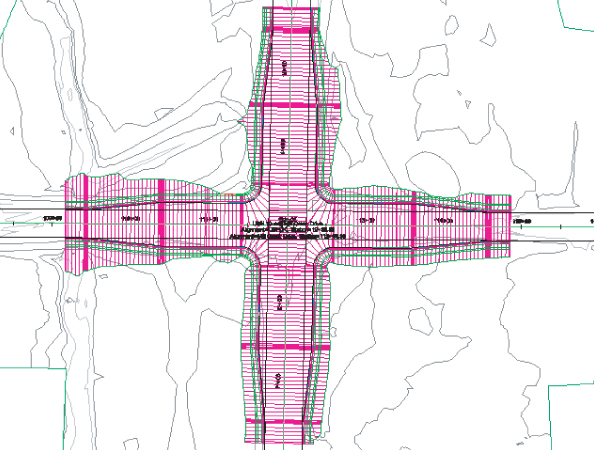
After a few moments of processing, you will see a corridor appear at the intersection of the roads. Use the REGEN command if you do not see the frequency lines. Your corridor should now resemble Figure 11.37.

Figure 11.37 The nearly completed intersection

12. Select the corridor and from the Corridor contextual tab ⇒ Modify Corridor panel, select Corridor Properties.

13. Switch to the Parameters tab of the Corridor Properties dialog and highlight one of the regions in the listing, as shown in Figure 11.38.

Figure 11.38 The best way to modify regions is using the corridor properties. The selected region will highlight graphically.

Notice how the region highlighted in the Parameters tab is outlined in the graphic. This will help you determine which region to edit, even in the largest of corridors.

To move from region to region without searching through the somewhat daunting list, use the Select Region From Drawing button.

In the next steps you will leverage the work Civil 3D has done for you and extend the intersection in all four directions.

14. Change the region start station on the west side of Mill Creek Road to 101+00 (3+200 for metric users).

15. Change the east side end station to 121+00 (3+700 for metric users).

16. Change the start station of the south end of USH 10 to 10+00 (0+300 for metric users).

17. Change the north side end station to 16+50 (0+500 for metric users).

18. Click OK and rebuild the corridor.

When the corridor is complete, it will look like Figure 11.39.

Figure 11.39 The completed intersection

Manually Modeling an Intersection

In some cases, you may find it necessary to model an intersection manually. Five-way intersections and intersections containing superelevated curves can't be created with the automated tools alone. You need to understand what the intersection tool is doing behind the scenes before you can be a true corridor guru. The next example will take you through an overview of the manual steps.

At the point where the example begins, a few pieces are already in place: the centerline alignments and profiles, EOP alignments and profiles, and the full road assemblies. The corridor for the intersection is started for you, but it contains only one baseline. For simplicity's sake, daylight subassemblies have been omitted from this example.

In this example, you'll add a baseline for an intersecting road to your corridor:

1. Open the ManualIntersection.dwg (ManualIntersection_METRIC.dwg) file, which you can download from this book's web page.

2. Select the corridor and from the Corridor contextual tab ⇒ Modify Corridor panel, select Corridor Properties.

3. Switch to the Parameters tab and click Add Baseline.

The Create Corridor Baseline dialog opens.

4. Pick the Syrah Way alignment, and then click OK to dismiss the dialog.

5. Click in the Profile field on the Parameters tab of the Corridor Properties dialog.

The Select A Profile dialog opens.

6. Pick the Syrah Way FG profile, and then click OK to dismiss the dialog.

You now have a new baseline, but the region still needs to be added.

7. In the Corridors Properties dialog, right-click BL – Syrah Way and select Add Region.

8. In the Create Corridor Region dialog, select Full Road Section, and then click OK to dismiss the dialog.

9. Expand BL – Syrah Way by clicking the small + sign, and see the new region you just created.

10. Click OK to dismiss the Corridor Properties dialog and select the option to rebuild the corridor.

Once the corridor finishes rebuilding, it will look like Figure 11.40.

Figure 11.40 The Syrah Way baseline added

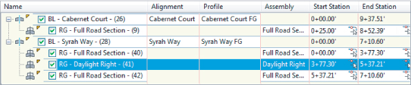
Notice that the region for the second baseline extends all the way through the intersection. You must now split the Syrah region to accommodate the curb returns.

11. Open the Corridor Properties dialog and switch to the Parameters tab. Select the RG-Full Road Section under the BL – Syrah Way – (10) baseline (number may vary), and then right-click and select Split Region.

12. Enter 377.3′ (115 m) and press to create the first region.

13. Enter 537.21′ (163.74 m) and press to form the second split.

14. Press again to return to the Corridor Parameters dialog.

15. Switch the middle subassembly to Daylight Right and then click OK.

Your corridor parameters will now match Figure 11.41.

Figure 11.41 Split the Syrah Way baseline into three regions to accommodate curb returns.

16. Click OK and, as always, choose to rebuild the corridor.

You will see that the way has been cleared for the curb assemblies to be applied, as shown in Figure 11.42.

Figure 11.42 The intersection corridor…so far

17. Save the drawing for use in the next exercise.

Creating an Assembly for the Intersection

You built several assemblies in Chapter 9, “Subassembly Composer,” but most of them were based on the paradigm of using the assembly marker along a centerline. This next exercise leads you through building an assembly that attaches at the EOP.

This exercise uses the LaneSuperelevationAOR subassembly (see Figure 11.43), but you're by no means limited to this subassembly in practice. You can use any lane subassembly that allows for a width and elevation target such as BasicLaneTransition, GenericPavementStructure, or LaneOutsideSuperWithWidening. Be sure the previous exercise is complete before proceeding.

Figure 11.43 An assembly for an intersection curb return

To create an assembly suitable for use on the filleted alignments of the intersection, follow these steps:

Your assembly should now look like Figure 11.43.

Adding Baselines, Regions, and Targets for the Intersections

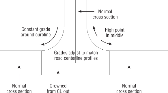
The Intersection assembly attaches to alignments created along the EOP. Because a baseline requires both horizontal and vertical information, you also need to make sure that every EOP alignment has a corresponding finished ground (FG) profile.

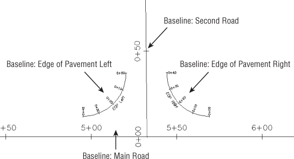
It may seem awkward at first to create alignment and profiles for things like the EOP, but after some practice you'll start to see things differently. If you've been designing intersections using 3D polylines or feature lines, think of the profile as a vertical representation of a feature line and the profile grid view as the feature-line elevation editor. If you've designed intersections by setting points, think of alignment PIs and profile PVIs as points. If you need a low point midway through the EOP, as indicated in the sketch at the beginning of this section, you'll add a PVI with the appropriate elevation to the EOP FG profile.

To avoid getting confused by multiple targets, baselines, and regions, here are a few tips:

Using Multiple Targets

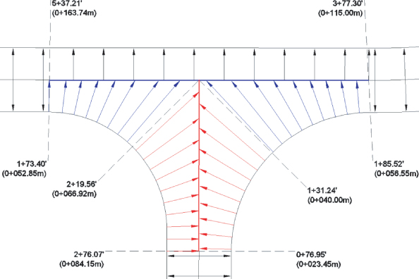
Civil 3D allows you to select more than one item in Width Or Offset Target and Slope Or Elevation Target areas. You can use any number of targets. You can even mix and match the types of targets you use, such as alignments with polylines, survey figures, and feature lines.

In the example that follows, you need two alignment targets and two profile targets in each curb region. To help Civil 3D figure out what you want, you need to verify that it will use the target that it finds first as it radiates out from the baseline. In most cases, you can click the Target To Nearest Offset option found in the target selection dialogs.

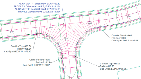
In the following graphic, the arrows represent the assemblies seeking out a target. From station 1+73.40 (0+052.85 for metric users) to 2+19.56 (0+066.92 for metric users), the Syrah Way alignment is closer to the west curb baseline; therefore, Syrah Way's geometry is used as the target. From station 2+19.56 (0+066.92 for metric users) to 2+76.07 (0+084.15 for metric users), Cabernet Court's alignment is closer and is used as the target.

---

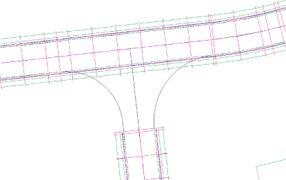
You'll finalize the corridor intersection in the next exercise. Along the way, you'll examine the corridor in various stages of completion so that you'll understand what each step accomplishes. In practice, you'll likely continue working until you build the entire model. Make sure you've completed the last two exercises, and then follow these steps:

1. Continue working in your drawing from the previous exercise (ManualIntersection.dwg or ManualIntersection_METRIC.dwg).

2. (Optional) Zoom to the area where the profile views are located. Notice that existing and proposed ground profiles are created for both EOP alignments (see Figure 11.44). The step of developing the design profiles has been completed for you.

Figure 11.44 The Parameters tab with a new baseline and region

3. Select the corridor, and then open the Corridor Properties dialog and switch to the Parameters tab.

4. Click Add Baseline.

The Create Corridor Baseline dialog opens.

5. Select the Cab-Syrah EOP W alignment, and click OK.

6. Click in the Profile field on the Parameters tab of the Corridor Properties dialog where it says <Click here…>.

7. In the Select A Profile dialog, select Cab-Syrah EOP W - FG, and click OK.

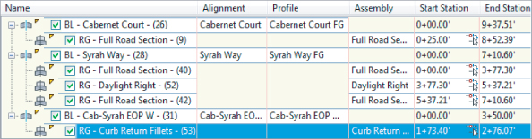
8. Right-click baseline BL – Cab-Syrah EOP W and select Add Region. (Your numbering may differ from that shown in Figure 11.44.)

9. In the Create Corridor Region dialog, select Curb Return Fillets, and then click OK to dismiss the dialog.

10. Click the small plus sign to expand the baseline, and see the new region you just created.

The Parameters tab of the Corridor Properties dialog will look like Figure 10.44.

11. Change the region start station to 1+73.40 (0+052.85 for metric users), and the region end station to 2+76.07 (0+084.15 for metric users).

These stations represent the PC and PT stations of the curb alignment.

12. Click OK to dismiss the Corridor Properties dialog and rebuild your corridor.

Your corridor should now look similar to Figure 11.45.

Figure 11.45 Your corridor after applying the Curb Return Fillets assembly

What is missing from the corridor? You need to set targets, and add more frequency lines along the curves. Of course, you will repeat the process on the east side of the road as well.

13. Select the corridor and from the Corridor Contextual tab ⇒ Modify Corridor, click Corridor Properties.

14. On the Parameters tab, set the frequency by clicking the ellipsis button in the Frequency column of the RG – Curb Return Fillets region row. Set both tangents and curves to 5′ (1 m). Click OK.

15. Click the ellipsis for targets of this region, and do the following:

A. Click the Width Alignment target for LaneSuperelevationAOR. Click the Select From Drawing button. Click both Syrah Way and Cabernet Court centerline alignments.

B. Press when complete.

C. In the Set Width Or Offset Target dialog, click Add. Both alignments will appear in the listing, as shown in Figure 11.46a.

Figure 11.46 In the Set Width Or Offset Target dialog, use the Select From Drawing button to pick both Syrah Way and Cabernet Court centerlines (left). In the Set Slope Or Elevation Target dialog, pick alignment first, and then add the FG profile (right)

D. Click OK when complete.

16. Click the Outside Elevation Profile target for LaneSuperelevationAOR, and do the following:

A. From the Select an Alignment drop-down, select Syrah Way from the list.

B. Highlight the Syrah Way FG profile and click Add.

C. Change the selected alignment to Cabernet Court.

D. Highlight the Cabernet Court FG profile and again click Add.

Both profiles will appear in the listing, as shown in Figure 11.46b.

E. Click OK.

17. Click OK to dismiss target mapping, and click OK to let the corridor rebuild.

Your intersection should now look like Figure 11.47.

Figure 11.47 Three baselines completed — one to go

18. Repeat steps 4–17 for the Cab-Syrah EOP E.

Here are some hints to get you going: The region should go from station 0+76.95 (0+023.45 for metric users) to 1+85.52 (0+056.54 for metric users). The frequency should be 5′ (1 m) for both tangents and curves. The target mapping will be identical to the region you created in steps 15 and 16.

19. Let the corridor rebuild one last time and admire your work.

The completed intersection should look like Figure 11.48.

Figure 11.48 The completed intersection

Troubleshooting Your Intersection

The best way to learn how to build advanced corridor components is to go ahead and build them, make mistakes, and try again. This section provides some guidelines on how to “read” your intersection to identify what steps you may have missed.

Your lanes appear to be backward.

Occasionally, you may find that your lanes wind up on the wrong side of the EOP alignment, as in Figure 11.49. The most common cause is that your assembly is backwards from what is needed based on your alignment direction.

Figure 11.49 An intersection with the lanes modeled on the wrong side

Fix this problem by editing your subassembly to swap the lane to the other side of the assembly. If the assembly is used in another region that is correct, just make a new assembly that is the mirror reverse of the other assembly and apply the new one to the alignment.

Since so many design elements rely on the alignment as their base, it is better to add a new assembly rather than reversing the direction of the alignment.

Your intersection drops down to zero.

A common problem when modeling corridors is the cliff effect, where a portion of your corridor drops down to zero. You probably won't notice in plan view, but if you rotate your corridor in 3D using the Object Viewer (see Figure 11.50), you'll see the problem. The most common cause for this phenomenon is incorrect region stationing.

Figure 11.50 A corridor viewed in 3D, showing a drop down to zero

Fix this problem by making sure your baseline profile exists where you need it, and make note of the station range. Set your station range in the corridor to be within the correct range.

Your lanes extend too far in some directions.

There are several variations on this problem, but they all appear similar to Figure 11.51. All or some of your lanes extend too far down a target alignment, or they may cross one another, and so on.

Figure 11.51 The intersection lanes extend too far down the main road alignment.

This occurs when a target alignment and profile have been omitted for one or more regions. In the case of Figure 11.51, the EOP Left baseline region was only set to one alignment. In an intersection, you need two targets in a corner region to model the road correctly.

Your lanes don't extend far enough.

If your intersection or portions of your intersection look like Figure 11.52, you neglected to set the correct target alignment and profile.

Figure 11.52 Intersection lanes don't extend out far enough.

You can fix this problem by opening the Target Mapping dialog for the appropriate regions and double-checking that you assigned targets to the right subassembly. It's also common to accidentally set the target for the wrong subassembly if you use Map All Targets, or if you have poor naming conventions for your subassemblies.

Checking and Fine-Tuning the Corridor Model

Recall that the EOP profiles are developed by creating a preliminary corridor surface model. To create the EOP elevations, you filled in the gaps by creating the EOP design profile where the preliminary surface stops and then picks back up again on the adjacent road (or in the case of the cul-de-sac, the opposite side of the street).

You will want to check the elevations of the corridor model against the profiles you created. The preliminary surface model was a best guess for elevations; now you need to reconcile your corridor geometry with those best-guess profiles. Figure 11.53 shows a common elevation problem that arises in the first iteration of intersection design.

Figure 11.53 A potential elevation problem in the intersection

The first step in correcting this is creating a corridor surface model out of Top links. The surface will show you exactly how Civil 3D is interpreting your design, elevation-wise.

Before beginning this exercise, review the basic corridor surface building sections in Chapter 10. When you think you are ready, follow these steps:

The next exercise will lead you through placing some design labels to assist in perfecting your model, and then show you how to easily edit your EOP FG profiles to match the design intent on the basis of the draft corridor surface built in the previous section.

Don't forget a few basics that will help you navigate this exercise easier. If you wish to see the drawing without the corridor, then freeze the corridor layer, which is C-ROAD-CORR. Don't forget to thaw this layer when you need it later! You can change the view of your surface around by changing the surface style. Also, remember that display order may be an issue. You will have corridor feature lines overlapping alignments, so it may be best to use the Send To Back option on the corridor.

1. Continue working in ManualFineTune.dwg (ManualFineTune_METRIC.dwg) from the previous exercise.

2. For the next few steps, either freeze the corridor layer or send your corridor display order to the back.

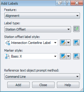
3. From the Annotate tab on the ribbon ⇒ Labels & Tables panel, click the Add Labels button.

The Add Labels dialog will appear.

4. Set Feature to Alignmentand Label Type to Station Offset.

5. Set Station Offset Label Style to Intersection Centerline Label, as shown in Figure 11.54.

Figure 11.54 Add alignment labels to identify potential problem areas.

6. Set Marker Style to Basic X, and click Add.

This label reference two alignments and two profiles.

7. The command line will read Select Alignment:. Click Syrah Way.

8. The command line will read Specify station along alignment:. Use object snaps to specify the intersection of Syrah Way and Cabernet Court.

9. At the Specify station offset: prompt, type 0 (zero) and press .

10. At the Select profile for label style component Profile 1: prompt, right-click to bring up a list of profiles and choose Syrah Way FG.

11. Click OK to dismiss the dialog.

12. At the Select alignment for label style component Alignment 2: prompt, pick the Cabernet Court alignment.

13. At the Select profile for label style component Profile 2: prompt, right-click to open a list of profiles, and choose Cabernet Court FG.

14. Click OK to dismiss the profile listing, and press Esc to exit the labeling command.

15. Pick the label, and use the square-shaped grip to drag the label somewhere out of the way.

Keep the Add Labels dialog open for the next part of the exercise.

This label shows you that the crown elevations of the Cabernet Court FG and Syrah Way FG are both equal to 811.204′ (247.255 m), which is great! If they differed at all, you'd have some adjustments to make on the FG profiles where the roads meet.

The next part of the exercise guides you through the process of adding a label to help determine what elevations should be assigned to the start and end stations of the EOP Right and EOP Left alignments.

16. In the Add Labels dialog, change the feature to Surface and Label Type to Spot Elevation, and click Add.

This label compares proposed surface elevation and the corresponding profile elevation.

17. At the Select a Surface <or press enter to select from list>: prompt, pick any contour from the corridor surface.

18. At the Select a Point: prompt, use your Endpoint osnap to pick the PC station of the right curb alignment.

19. At the Select surface for label style component Surface2: prompt, press .

20. Highlight Prelim, and click OK.

21. At the Select alignment for label style component Alignment: prompt, press .

22. Highlight Cab-Syrah EOP W and click OK. Remain in the command.

The question marks that initially came in with the label should now show the elevation differences between proposed and Prelim elevation at the station of interest.

23. Place another label at the PT station.

Because you have already specified the surface and profile, the label will pop right in.

24. Press Esc and click Add in the Add Labels dialog.

You need to stop and start the command to switch the alignment used in the label.

25. Using the same techniques you used on the west side of the road, add labels at the PC and PT stations of Cab-Syrah EOP E.

26. Select the labels. Click and drag the square grip and add leaders to make them easier to read.

Your labels should look like Figure 11.55.

Figure 11.55 The corridor with all labels placed

27. Save the drawing for use in the next exercise.

As you can observe from the labels, the profiles and the surface model are perfect except for station 1+73.40 (0+052.85 for metric users) along Cab-Syrah EOP W. In fact, if the elevation difference doesn't bother you, you can skip the next steps. If you want your design to be as perfect as it can be, carry on:

1. Continue working in ManualFineTune.dwg (ManualFineTune_METRIC.dwg) from the previous exercise.

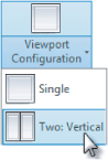
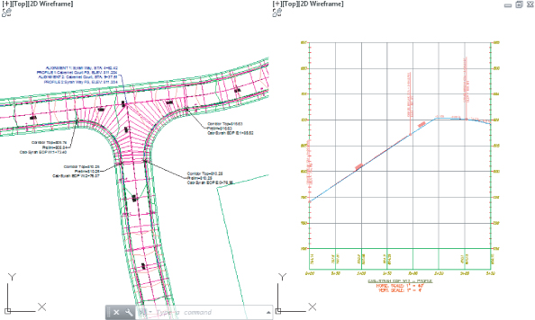
2. Split your model space into two views for easier working: Go to the View tab ⇒ Model Viewports panel and select Viewport Configuration ⇒ Two: Vertical.

Pan in the drawing to show the profile view for CAB-Syrah EOP W. Your screen should look similar to Figure 11.56.

Figure 11.56 Use a split screen to see the plan and profile simultaneously.

3. Pick the Cab-Syrah EOP W – FG profile (the blue line in the profile view), and from the contextual Ribbon, click Geometry Editor.

4. On the Profile Layout Tools toolbar, click Insert PVIs-Tabular.

5. In the Insert PVIs dialog, set the vertical curve type to None.

6. Type 173.4′ (52.85 m) for the station. (Station notation is not needed.) Type 804.84′ (245.62 m) for the elevation. Click OK.

7. Select the corridor and choose Rebuild Corridor from the contextual tab.

Your first curb return label will now report a perfect match between the Corridor Surface elevation and the FG Profile elevation (Figure 11.57).

Figure 11.57 Add PVI stations and elevations to match the desired FG elevations.

8. Pick the Corridor Top surface, and use the Object Viewer to study the TIN in the intersection area.

Study the contours in the intersection area. You may wish to add feature lines as breaklines to the surface model, as you learned in Chapter 10.

When Automatic Surface Boundaries Are Not Available

You will come to a point in the corridor modeling where you need to add a corridor surface boundary, but the best options (Add Automatically ⇒ Daylight or Corridor Extents As Outer Boundary) are not available. There will also be situations where Corridor Extents As Outer Boundary does not go where you want it to go. In those situations, you will need to use the Add Interactively tool.

Add Interactively allows you to direct Civil 3D to use the correct feature line as the boundary. You will trace your desired outer bounds with a temporary graphic called a jig.

1. Open the Concord Commons Corridor.dwg (Concord Commons Corridor_METRIC.dwg) file, which you can download from the book's web page.

You will see a surface in this file that needs some serious reining in.

2. Select the corridor, and click Corridor Properties on the contextual Ribbon. Select the Boundaries tab.

3. Right-click on the Corridor Topsurface and select Corridor Extents as the outer boundary. Click OK and rebuild the corridor.

4. Pan around the drawing.

The contours are tidier, but the surface inside the loop formed by Frontenac Drive has not been cleaned up. In the next steps of the exercise, you will clean up the surface using the Add Interactively tool.

5. Set your AutoCAD object snaps to use only Endpoint and Nearest.

These will be the most helpful osnaps to steer Civil 3D in the right direction.

6. In the Corridor Properties dialog ⇒ Boundaries tab, right-click Concord Commons Corridor Top and select Add Interactively.

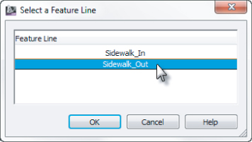
7. Start near station 0+00 (0+000 for metric users) on the inside of the loop and click the Sidewalk_Out feature line. Trace it with your cursor.

8. When the jig is going to the correct location, click to commit the boundary.

The following image shows what the jig will look like:

As you move around, you will see the jig tends to move unexpectedly at region boundaries. Steer the jig where you want it to go by clicking and tracing. If you made a mistake, type U for undo at the command line.

If you click a location where there is more than one feature line, or you are zoomed out to where your pickbox encompasses two lines, you will see a dialog like this one asking you to pick the line you are after:

9. After you have finally come back around to where you started the boundary, type C (for close) at the command line, and press .

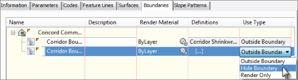
10. When you complete the inner loop and return to the Corridor Properties dialog, set the Corridor Boundary (2) boundary type to Hide Boundary, as shown here. Click OK and rebuild the corridor.

Yes, this process can be tedious. However, your work will pay off when changes are made to your design. These boundaries are dynamic to the design, unlike a polyline boundary.

---

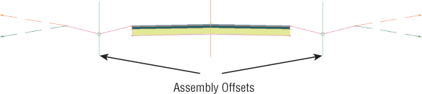
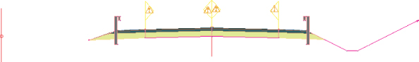
Using an Assembly Offset

In Chapter 10, “Basic Corridors,” you completed a road-widening example with a simple lane transition. Earlier in this chapter, you worked with a roadside-ditch transition, intersections, and cul-de-sacs. These are just a few of the techniques for adjusting your corridor to accommodate a widening, narrowing, interchange, or similar circumstances. There is no single method for building a corridor model; every method discussed so far can be combined in a variety of ways to build a model that reflects your design intent.

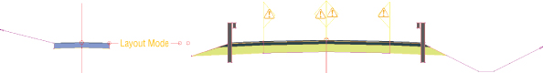
Another tool in your corridor-building arsenal is the assembly offset. In Chapter 10, you had your first glimpse of an offset assembly, but in the example that follows you will have a chance to use one for a bike path design.

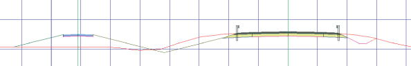
Notice in Figure 11.58 how the frequency lines in the corridor are running perpendicular to the main alignment. The bike path is an alignment that is not a constant offset through the length of the corridor. In this scenario, the cross section of the bike path itself is skewed. This could prove problematic when computing end area volumes for the bike path pavement. This is the result of using an assembly where all of the design is based off one main baseline assembly.

Figure 11.58 A bike path modeled with a traditional assembly

There are several advantages to using an offset assembly instead. The offset assembly requires its own alignment and profile for design. In the corridor that results, a secondary set of frequency lines is generated perpendicular to the offset alignment, as shown in Figure 11.59. Additionally, you can use a marked point assembly to model the ditch between the bike path and the main road.

Figure 11.59 Modeling a bike path with an assembly offset

There are many uses of offset assemblies besides bike paths. Typical examples of when you'll use an assembly offset include transitioning ditches, divided highways, and interchanges. The assembly in Figure 11.60, for example, includes two assembly offsets. The assembly could be used for transitioning roadside swales, similar to the first exercise in this chapter.

Figure 11.60 An assembly with two offsets representing roadside swale centerlines

When you use an assembly using an offset in your corridor, you must assign an alignment and profile to it. The only restriction to the offset assembly is that it can't use the same alignment or profile as the main part of the assembly. In the case where you want your offsets to follow the same elevation, you will need to use the Superimposed Profile tool to effectively make a copy of the desired profile.

In this exercise, you will model a bike path with an assembly offset:

1. Open the HWY10-BikePath.dwg (HWY10-BikePath_METRIC.dwg) file, which you can download from this book's web page.

2. Zoom to the area of the drawing where the assemblies are located.

You'll see an incomplete assembly called Road With GR And Bikepath.

3. Click on the main assembly marker, and then from the contextual Ribbon tab, click Add Offset in the Modify Assembly panel.

4. At the Specify offset location: prompt, click to the left of the Road With GR And Bikepath assembly, leaving enough room for the bike lane and ditch.

Your result should look like Figure 11.61. The warning symbols indicate that you can no longer use the assembly for roads where superelevation occurs at points other than the centerline. Superelevation at the crown will still work, which is the situation used here.

Figure 11.61 Road With GR And Bikepath assembly, so far

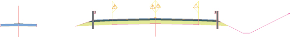
5. Open the Civil Imperial Subassembly tool palette.

6. Switch to the Basic tab, and select the BasicLane subassembly.

7. In the Advanced Parameters in the Properties dialog, set Side to Right and Width to 5′ (1 m).

8. Click to place the subassembly on the offset assembly, and click the offset assembly again to form the left side.

Your assembly should now look like Figure 11.62.

Figure 11.62 Road With GR And Bikepath assembly with the BasicLane as a bike path

Next, you will use a MarkPoint assembly to set the stage for building a ditch between the bike path and the main road.

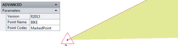
9. Switch to the Generic tab in the subassemblies tool palette, and click the MarkPoint subassembly.

10. Change the Point Name to BIKE (use all capital letters).

11. Click on the outermost point of the left shoulder subassembly.

Your marker will look like Figure 11.63.

Figure 11.63 A close-up of the MarkPoint subassembly

12. From the Generic tab of the Subassemblies tool palette, click the LinkSlopesBetweenPoints subassembly, and do the following:

A. Set Marked Point Name to BIKE (again, use all capital letters).

B. Set Ditch Width to 0.5′ (0.15 m).

C. Click on the right side of the bike path.

The offset assembly will now look like Figure 11.64.

Figure 11.64 The LinkSlopesBetweenPoints subassembly in layout mode

13. Add a LinkSlopeToSurface generic link subassembly, and do the following:

A. Set the Side to Left and Slope to 25%.

B. Place the subassembly on the left side of the bike path. Press Esc to complete adding subassemblies and save the drawing.

The completed assembly will look like Figure 11.65.

Figure 11.65 The completed assembly with offset

Next, you will create a corridor using this new assembly. You need to have completed the previous exercise before proceeding.

Figure 11.66 Inside the corridor Section Editor

Don't forget to close the Section Editor before closing the drawing!

The Trouble with Bowties

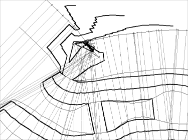
In your adventures with corridors, chances are pretty good that you'll create an overlapping link or two. These overlapping links are known not-so-affectionately as bowties. Here's an example:

Bowties are problematic for several reasons. In essence, the corridor model has created two or more points at the same x and y locations with a different z, making it difficult to build surfaces, extract feature lines, create a boundary, and apply codeset styles that render or hatch.

When your corridor surface is created, the TIN has to make some assumptions about crossing breaklines that can lead to strange triangulation and incoherent contours, such as in the following graphic:

When you create a corridor that produces bowties, the corridor won't behave as expected. Choosing Corridors ⇒ Utilities to extract polylines or feature lines from overlapping corridor areas yields an entity that is difficult to use for additional grading or manipulation because of extraneous, overlapping, and invalid vertices. If the corridor contains many overlaps, you may have trouble even executing the extraction tools. The same concept applies to extracted alignments, profiles, and COGO points.

If you try to add an automatic or interactive boundary to your corridor surface, either you'll get an error or the boundary jig will stop following the feature line altogether, making it impossible to create an interactive boundary.

To prevent these problems, the best plan is to try to avoid link overlap. Be sure your baseline, offset, and target alignments don't have redundant or PI locations that are spaced excessively close.

If you initially build a corridor with simple transitions that produce a lot of overlap, try using an assembly offset and an alignment besides your centerline as a baseline. Another technique is to split your assembly into several smaller assemblies and to use your target assemblies as baselines, similar to using an assembly offset. This method was used to improve the river corridor shown in the previous graphics. The following graphic shows the two assemblies that were created to attach at the top of bank alignments instead of the river centerline:

The resulting corridor is shown here:

The TIN connected the points across the flat bottom and modeled the corridor perfectly, as you can see in the following image:

Another method for eliminating bowties is to notice the area where they seem to occur and then adjust the regions. If your daylight links are overlapping, perhaps you can create an assembly that doesn't include daylighting and create a region to apply that new assembly.

If overlap can't be avoided in your corridor, don't panic. If your overlaps are minimal, you should still be able to extract a polyline or feature line — just be sure to weed out vertices and clean up the extracted entity before using it for projection grading. You can create a boundary for your corridor surface by drawing a regular polyline around your corridor and adding it as a boundary to the corridor surface under the Surfaces branch in Prospector. The surface-editing tools, such as Swap Edge, Delete Line, and Delete Point, can also prove useful for the final cleanup and contour improvement of your final corridor surface.

As you gain more experience building corridors, you'll be able to prevent or fix most overlap situations, and you'll also gain an understanding of when they aren't having a detrimental effect on the quality of your corridor model and resulting surface.

---

Using a Feature Line as a Width and Elevation Target

You've gained some hands-on experience using alignments and profiles as targets for swale, intersection, and cul-de-sac design. Civil 3D adds options for corridor targets beyond alignments and profiles. You can use grading feature lines, survey figures, or polylines to drive horizontal and/or vertical aspects of your corridor model.

Imagine using an existing polyline that represents a curb for your lane-widening projects without duplicating it as an alignment, or grabbing a survey figure to assist with modeling an existing road for a rehabilitation project. The next exercise will lead you through an example where a lot-grading feature line is integrated with a corridor model:

1. Open the Feature Line Target.dwg (Feature Line Target_METRIC.dwg) file, which you can download from this book's web page.

This drawing includes a completed assembly and a partially completed corridor. You task will be to use the yellow feature lines that run through the project as targets in the corridor.

2. Zoom to the corridor and select it. From the Corridor contextual tab ⇒ Modify Corridor panel, choose Corridor Properties.

3. Switch to the Parameters tab in the Corridor Properties dialog.

4. Click the ellipsis button in the Targets field in the RG-Subdivision region. Note that the number following the region will vary. The higher the number, the more previous attempts at building the corridor the authors have made before handing the drawing over to you.

The Target Mapping dialog appears.

5. Click the <None> field next to Target Alignment for the Slope - Left subassembly.

The Set Width Or Offset Target dialog appears.

6. Choose Feature Lines, Survey Figures And Polylines from the Select Object Type To Target drop-down list (see Figure 11.67).

Figure 11.67 The Select Object Type To Target drop-down list as seen in both the Set Width Or Offset Target and Set Slope Or Elevation Target dialogs

7. Click the Select From Drawing button, and when you see the command-line prompt Select feature lines, survey figures or polylines to target:, select the yellow feature line to the north of the alignmentand then press .

The Set Width Or Offset Target dialog reappears, with an entry in the Selected Entries To Target area.

8. Click OK to return to the Target Mapping dialog.

If you stopped at this point, the horizontal location of the feature line would guide the Slope-Left subassembly, and the vertical information would be driven by the slope set in the subassembly properties. Although this has its applications, most of the time you'll want the feature line elevations to direct the vertical information. The next few steps will teach you how to dynamically apply the vertical information from the feature line to the corridor model.

9. In the Slope or Elevation Targets section, click the <None> field next to Target Profile for the Slope-Left subassembly.

The Set Slope Or Elevation Target dialog appears.

10. Make sure Feature Lines, Survey Figures And Polylines is selected in the Select Object Type To Target drop-down.

11. Click the Select From Drawing button, and when you see the command-line prompt Select feature lines, survey figures or 3D polylines to target:, select the yellow feature line to the north again and then press .

The Set Slope Or Elevation Target dialog reappears, with an entry in the Selected Entries To Target area.

12. Click OK to return to the Target Mapping dialog.

13. Click OK to return to the Corridor Properties dialog.

14. Repeat steps 3–10 for Slope - Right on the right side of the corridor using the feature line to the south of the alignment.

15. Click OK to exit the Corridor Properties dialog and choose rebuild corridor.

The corridor will rebuild to reflect the new target information and should look similar to Figure 11.68.

Figure 11.68 The corridor now uses the grading feature lines as width and elevation targets.

Once you've linked the corridor to this feature line, any edits to this feature line will be incorporated into the corridor model. You can establish this feature line at the beginning of the project and then make horizontal edits and elevation changes to perfect your design. The next few steps will lead you through making some changes to this feature line and then rebuilding the corridor to see the adjustments.

16. Select the corridor, right-click, and choose Display Order ⇒ Send To Back.

Doing so sends the corridor model behind the target feature line.

17. Select one of the feature lines so that you can see its grips. Experiment with the feature lines by moving several grips.

18. Select the corridor, and then right-click and choose Rebuild Corridor.

The corridor will rebuild to reflect the changes to the target feature lines.

Edits to targets — whether they're feature lines, alignments, profiles, or other Civil 3D objects — drive changes to the corridor model, which in turn drives changes to any corridor surfaces, sections, section views, associated labels, and other objects that are dependent on the corridor model.

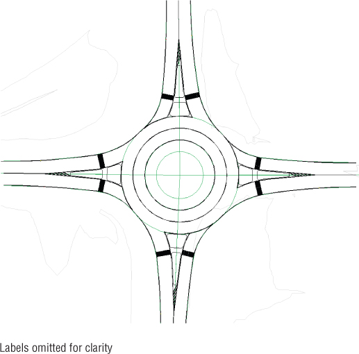
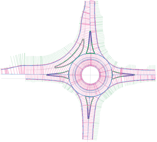
Roundabouts: The Mount Everest of Corridors

If you really understand what went on earlier in this chapter, you are almost ready for roundabout design. You may want to wait to tackle your first roundabout until after reading Chapter 16, “Grading.”

The same concepts apply to a roundabout as for a standard road junction, but you will have several more regions, baselines, and corresponding profiles.

This section will help you prepare files for roundabout design. This section will not take you through every detail of corridor creation, but once you master the topics of intersection design, a roundabout is an extension of the same concepts.

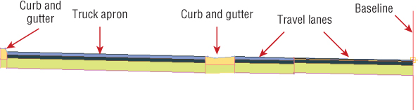
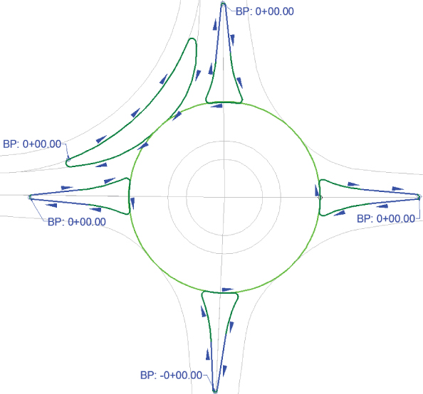
A roundabout is best done in several corridors:

Drainage First

Based on your existing ground surface, determine the general direction that you want water to flow away from the center of the roundabout. Use grading tools and a feature line to create the general drainage direction of the roundabout.

Chapter 16 will go into much more depth on creating grading. You will certainly want to have an understanding of grading basics before you tackle a roundabout.

Create a feature line that represents the highest elevations. In the example shown in Figure 11.69, the feature line slopes downward and acts as a ridge to separate water flow. The grading tools are then used to create grading objects and a corresponding surface model called “Roundabout Grading.”

Figure 11.69 Feature lines and grading create a preliminary surface to ensure proper drainage through the roundabout.

The Roundabout Grading surface will be the basis for our profile elevations through the rest of the design process.

Roundabout Alignments

Roundabouts need alignments to guide the design for the same reasons that an intersection needs them. Alignments will be baselines and targets for the approaches and rotary. Create alignments manually with the tools you learned earlier in this chapter, or start with the handy roundabout layout tool.

The roundabout layout tools create horizontal data based on the location of the center of the roundabout and the approach alignments.

In the exercise that follows, you will create the Civil 3D alignments needed to create a roundabout:

1. Open the Roundabout Layout.dwg (Roundabout Layout_METRIC.dwg) file, which you can download from this book's web page.

2. From the Home tab ⇒ Create Design panel, select Intersections ⇒ Create Roundabout, as shown in Figure 11.70.

Figure 11.70 Access the Create Roundabout tool from the Home tab.

3. At the Specify roundabout centerpoint: prompt, use your Intersection osnap to select the point where the approaches meet.

4. At the Select approach road: prompt, select all four alignments leading into the roundabout, and press when you are done.

You now see the Create Roundabout – Circulatory Road screen, shown in Figure 11.71.

Figure 11.71 The first roundabout layout screen for designing the main circulatory road

5. Verify that you are using the correct standards for your units. Click on the ellipsis next to the Roundabout Design Standard File field, and verify that you are using the correct XML standards file.

A. If it is set correctly, click Cancel and continue to step 6.

B. If it is not set correctly, browse to the C:ProgramDataAutodeskC3D 2013enuDataCorridor Design Standards folder. Browse to either the Imperial or metric units folder and select the correct roundabout presets XML file. Click Open to return to the Create Roundabout dialog.

6. From the Predefined Parameters To Import drop-down, choose R=75 (Rg=25m).

This will be the radius from the center of the roundabout to the outermost circular edge of pavement.

7. Set Alignment Layer to C-ROAD and Alignment Label Set to Major And Minor Only. Click Next.

Now, you'll design the approach road exit and entry geometry. The options in the Create Roundabout – Approach Roads screen (see Figure 11.72) can be set independently for each approach, or you can click Apply To All, which will set the geometry for all four approaches.

Figure 11.72 Approach road widths at entry and exit

8. Set Predefined Parameters To Import to R=75 (Rg=25m). For Alignment Label Set, choose Major And Minor Only. Leave all other settings at their defaults.

9. Click the Apply To All button, and click Next.

10. In the Create Roundabout – Islands screen (see Figure 11.73), again set Predefined Parameters To Import to R=75 (Rg=25m).

Figure 11.73 Roundabout Islands parameters

11. Click Apply To All, and then click Next.

The final screen of the Create Roundabout wizard deals with pavement markings and signage. Notice that you can specify your own blocks for the signs that will be placed in this process.

Everything created in this last step is an AutoCAD polyline or block. The polylines have a global width set to indicate pavement marking thicknesses. These thicknesses are set in the Markings And Signs screen (Figure 11.74).

Figure 11.74 Pavement markings galore!

12. Leave all defaults in the Create Roundabout – Markings And Signs screen (Figure 11.74), and click Finish.

Your roundabout should resemble Figure 11.75. Since standards vary by region, the metric drawing will have slightly different default pavement markings.

Figure 11.75 Completed roundabout alignment layout

Finally, you will add a turn lane in the NW quadrant of the roundabout. When you're creating slip turn lanes, remember that the turn radius must be large enough to fillet the exit and entry roads without overlapping the other alignments.

When selecting the approach entry and exit alignments, you need to click the shorter approach alignments created by Civil 3D rather than the original approach road. For this reason, the exercise has you select inside the islands, just to be sure.

13. From the Home tab ⇒ Create Design panel, select Intersections ⇒ Add Turn Slip Lane.

14. When prompted to select the entry approach, select the north approach alignment inside the curb island.

15. When prompted for the exit approach, select the west approach alignment inside the curb island, as shown in Figure 11.76.

Figure 11.76 Entry and exit approach alignments for the slip lane

16. In the Draw Slip Lane screen shown in Figure 11.77, set the lane width to 14′ (4 m) and the radius to 150′(45 m).

Figure 11.77 Adding a slip lane

17. For the alignment layer, choose C-ROAD and for Alignment Label Set, choose Major And Minor Only. Click OK.

Your roundabout will now look like Figure 11.78.

Figure 11.78 The completed slip lane alignments

18. Save and close the drawing.

You now have all the alignments you need to start your roundabout design. At this point, you can add geometry to the alignments and modify what Civil 3D has created for you.

The horizontal layout is complete, but the roundabout design is far from done. No vertical data has been created; that is up to you.

This is as far as we will take you in this book in regard to building a roundabout step-by-tedious-step. Rest assured, however, that if you have truly mastered corridors, the techniques for completing a roundabout are similar to that of any intersection.

The remainder of this chapter gives you an overview of how to accomplish the rest on your own.

Center Design

All profiles need to meet at the elevations inside the traveled way in the circular pavement area of the roundabout. Therefore, the main circle design comes first.

To see an example of a completed roundabout corridor, open the drawing RoundaboutExample_FINISHED.dwg or RoundaboutExample_METRIC_FINISHED.dwg. Use these examples as a guide to “reverse engineer” your own roundabouts when you've mastered other forms of intersections.

You can use any of the circular alignments created by Civil 3D as the basis for this step, as long as your assembly works with the design. Remember to make note of which direction the alignment goes, to ensure the assembly you create is not backwards.

Extract profiles for the main circle design from the Existing Ground and Roundabout Grading surfaces, as shown in Figure 11.79.

Figure 11.79 Extract surface profiles around the main circular alignment.

The assembly you create for this preliminary design will also be used in the main design. Decide which alignment will be used as the circular design basis, and create an assembly based on your alignment location and desired geometry, as shown in Figure 11.80.

Figure 11.80 Center assembly for roundabout

This assembly can be used in several steps of the process. First it is used in a preliminary corridor called RAB Center. It can also be recycled to be the centerpiece of your main corridor. In the example, the main circle alignment created by Civil 3D, Roundabout_OUTER_EDGE, was used as the baseline for this initial corridor. There are no targets or frequencies set in this corridor. Like the cul-de-sac example earlier in this chapter, this is a preliminary corridor, used to ensure that profiles from the approach roads tie in at the correct elevations.

In the example drawings, a Top link surface was created from the RAB Center corridor. At this point, the roundabout will resemble Figure 11.81.

Figure 11.81 Preliminary center corridor and surface

Profiles for All

You have all the preliminary surfaces in place, and you have all the alignments you need, so it is time to extract profiles from your various surfaces.

In the RoundaboutExample_FINISHED.dwg and RoundaboutExample_METRIC_FINISHED.dwg files, the surface profiles for all the approach alignments were created by sampling the existing ground, drainage surface, and preliminary RAB Center corridor surface. These profiles will look something like Figure 11.82.

Figure 11.82 Surface profiles needed for design

When you create your design, you will see all your design considerations in the profile views. No matter how you decide to tie into existing ground and slope upward toward the surface, your design must tie into the preliminary center surface, as shown in Figure 11.83.

Figure 11.83 Design profiles must tie into the center.

Use techniques you learned earlier in this chapter to assist you. Labels are an especially valuable tool for roundabouts. Keep your profile views organized, as you will have at least three for each approach. If you have a slip turn lane, you will have a profile for that as well.

Tie It All Together

Stretch your legs and go for more coffee. It is time to put this thing together into a completed corridor. When you model the corridor initially, ignore curb islands — you will add them as individual corridors in a later step.

A simple roundabout can be completed using as few as three assemblies. In our example, however, the slip turn lane necessitates a total of four assemblies. In addition to the RAB Center assembly you saw in Figure 11.80, you will need three more assemblies, as shown in Figure 11.84.

Figure 11.84 Assemblies needed for the main roundabout corridor

These assemblies will be tied to the EOP alignments and profiles as baselines, similar to a traditional intersection. Each quadrant of the roundabout will target at least two alignments and profiles, as shown in Figure 11.85.

Figure 11.85 Roundabout corridor regions and targets

Keep in mind the direction of your alignments. If you build the corridor in stages, check the corridor periodically to make sure it is building correctly.

Create a corridor surface from your completed roundabout lanes. You will likely have to use the Add Interactively tool to add the boundary correctly.

Finishing Touches

The median islands are the last parts to go on the corridor. You can create them using simple grading objects, but since this is a book about mastering skills, and this is a chapter about corridors, you should examine the dynamic way.

Create a simple assembly containing the curb and gutter for the curb islands. This will be the assembly that you use with the median corridors (Figure 11.86).

Figure 11.86 Simple assembly containing just the curb and gutter on the median islands

Each median island will need its own alignment. Take note of the direction of the alignments to make sure they are compatible with the curb island assembly. If necessary, change the direction of the alignments using the Reverse Direction tool in the Modify panel of the contextual Ribbon tab. Figure 11.87 shows the bypass island and north island with directions.

Figure 11.87 Several median island alignments with direction shown

The good news is that the elevation data for the medians is already complete. Your main corridor's surface will act as the profile for each individual median. This also means that once the curb return corridors are created, they will be dynamic to the main corridor. After these little corridors are created and surface model information has been obtained, you can set them to Rebuild – Automatic and forget all about them.

Extract a profile for all the curb return alignments from the Top link surface model from the main roundabout corridor, as shown in Figure 11.88. You do not need to see this profile in a view, so you can click OK to extract.

Figure 11.88 Extract the profile for medians from your main roundabout surface.

When the design roundabout corridors are complete and surfaces are made, the next step is to merge the surfaces together. Create a final surface model and paste the main roundabout design in first. After the main corridor is pasted in, paste the smaller median corridor surfaces (see Figure 11.89).

Figure 11.89 The completed roundabout

Your next step is to use the corridor fine-tuning techniques you learned earlier in this chapter to ensure your grades are correct and the design is correct. To see an example of a completed corridor using these steps, take a look at RoundaboutExample_FINISHED.dwg (RoundaboutExample_FINISHED_METRIC.dwg), which you can download from www.sybex.com/go/masteringcivil3d2013.

The Bottom Line