Chapter 7
Profiles and Profile Views
Profile information is the backbone of vertical design. The AutoCAD® Civil 3D® software takes advantage of sampled data, design data, and external input files to create profiles for a number of uses. Profiles will be an integral part of corridors, as we'll discuss in Chapter 10, “Basic Corridors.” In this chapter we'll look at using profile creation tools, editing profiles, and generating and editing profile views, and you'll learn ways to get your labels just so.
In this chapter, you will learn to:
- Sample a surface profile with offset samples
- Lay out a design profile on the basis of a table of data
- Add and modify individual entities in a design profile
- Apply a standard band set
The Elevation Element
The whole point of a three-dimensional model is to include the elevation element that's been missing for years on two-dimensional plans. But to get there, designers and engineers still depend on a flat 2D representation of the vertical dimension as shown in a profile view (see Figure 7.1).
Figure 7.1 A typical profile view of the surface elevation along an alignment

A profile is nothing more than a series of data pairs in a station, elevation format. There are basic curve and tangent components, but these are purely the mathematical basis for the paired data sets. In AutoCAD Civil 3D, you can generate profile information in one of the following four ways:
Sampling from a Surface
Sampling from a surface involves taking vertical information from a surface object every time the sampled alignment crosses a TIN line of the surface. This is perfect for generating a profile for the existing ground.
Using a Layout to Create a Profile
Using a layout to create a profile allows you to input design information, setting critical station and elevation points, calculating curves to connect linear segments, and typically working within design requirements laid out by a reviewing agency.
Creating a Profile from a File
Creating from a file lets you reference a specially formatted text file to pull in the station and elevation pairs. Doing so can be helpful in dealing with other analysis packages or spreadsheet tabular data.
Creating a Best Fit Profile
Similar to the ability to generate a best fit alignment that we discussed in Chapter 6, “Alignments,” you can also create a best fit profile. You may find yourself using this method when you are trying to generate defined geometry for an existing road.
This section looks at all four methods of creating profiles.
Surface Sampling
![]()
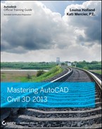
Working with surface information is the most elemental method of creating a profile. This information can represent any of the surfaces already in your drawing, such as an existing surface or any number of other surface-derived data sets. Surfaces can also be sampled at offsets, as you'll see in the next series of exercises. Follow these steps:
Figure 7.2 The drawing you'll use for this exercise
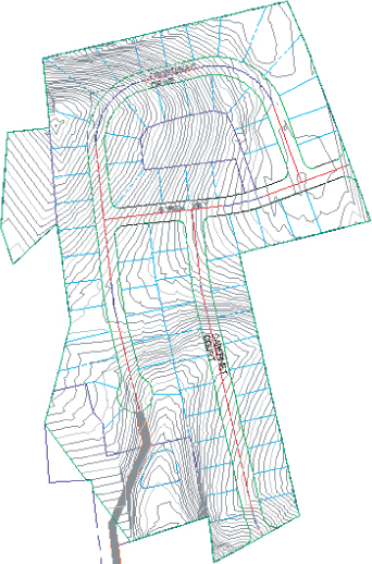

Figure 7.3 The Create Profile From Surface dialog
- The upper-right quadrant controls the selection of the surface that will be sampled as well as the offsets. You can select a surface from the list, or you can click the Pick On Screen button. Beneath the Select Surfaces box is a Sample Offsets check box. The offsets aren't applied in the left and right direction uniformly. You must enter a negative value to sample to the left of the alignment or a positive value to sample to the right. You can add multiple offsets in a comma-delimited list here, for example: -50, 25, -10, -5, 0, 5, 10, 25, 50. In all cases, whether or not you are sampling offsets, the profile isn't generated until you click the Add button.
- The Profile List box displays all profiles associated with the alignment currently selected in the Alignment drop-down menu. This area is generally static (it won't change), but you can modify the Update Mode, Layer, and Style columns by clicking the appropriate cells in this table. You can stretch and rearrange the columns to customize the view. The columns can only be modified in this location as they are created. Upon returning to the Create Profile From Surface dialog, the profiles previously created will have static values and can be changed in the Profile Properties dialog instead.
Figure 7.4 The Create Profile From Surface dialog with styles assigned on the basis of the Offset value

Figure 7.5 The Create Profile View – General wizard page

Figure 7.6 The Create Profile View – Station Range wizard page

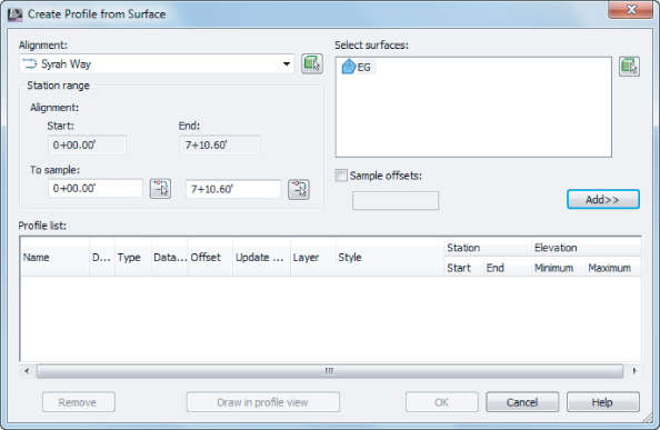
Figure 7.7 The Create Profile View – Profile View Height wizard page
Figure 7.8 The Create Profile View – Profile Display Options wizard page
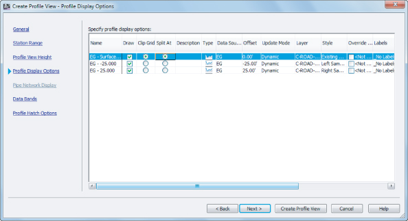
Figure 7.9 The Create Profile View – Data Bands wizard page
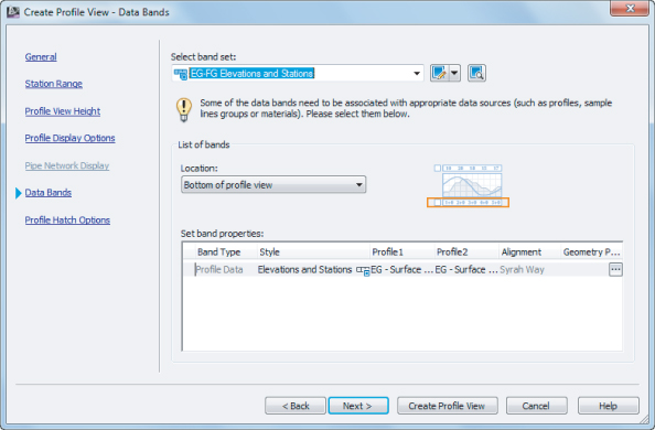
Figure 7.10 The complete profile view for Syrah Way
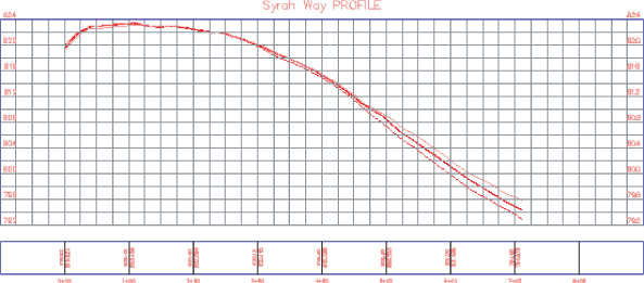
Figure 7.11 Alignment profiles on the Prospector tab
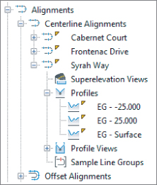
Figure 7.12 Splitting the screen for plan and profile editing
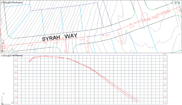
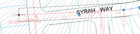
Figure 7.13 Grip-editing the alignment
By maintaining the relationships between the alignment, the surface, the sampled information, and the offsets, the software creates a much more dynamic feedback system for designers. This system can be useful when you're analyzing a situation with a number of possible solutions, where the surface information will be a deciding factor in the final location of the alignment. Once you've selected a location, you can use this profile view to create a vertical design, as you'll see in the next section.
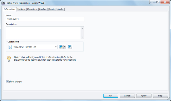
In the following short exercise you will generate a profile view which displays right to left:
You may need to move the profile view since the insert point of the profile view will now be in the lower-right corner instead of the lower-left corner as it was previously.
When this exercise is complete, you may close the drawing. A finished copy of this drawing is available from the book's website with the filename ProfileSampling_FINISHED.dwg or ProfileSampling_METRIC_FINISHED.dwg.
Changing a profile view style is straightforward, but because of the large number of settings in play with a profile view style, the changes can be dramatic. A profile view style includes information such as labeling on the axis, vertical scale factors, grid clipping, and component coloring.
Using various styles lets you make changes to the view to meet requirements without changing any of the design information associated with the profile. To learn more about editing and creating profile styles, refer to Chapter 21, “Object Styles.”
Layout Profiles
![]()
Working with sampled surface information is dynamic, and the improvement over previous generations of Autodesk® civil design software is profound. Moving into the design stage, you'll see how these improvements continue as you look at the nature of creating design profiles. By working with layout profiles as a collection of components that understand their relationships with each other as opposed to independent finite elements, you will realize the power of the AutoCAD Civil 3D software as a design tool in addition to being a drafting tool.
You can create layout profiles in two basic ways:
PVI-Based Layout
PVI-based layouts are the most common, using tangents between points of vertical intersection (PVIs) and then applying curve parameters to connect them. PVI-based editing allows editing in a more conventional tabular format.
Entity-Based Layout
Entity-based layouts operate like horizontal alignments in the use of free, floating, and fixed entities. The PVI points are derived from pass-through points and other parameters that are used to create the entities. Entity-based editing allows for the selection of individual entities and editing in an individual component dialog.
You'll work with both methods in the next series of exercises to illustrate a variety of creation and editing techniques. First, you'll focus on the initial layout, and then you'll edit the various layouts.
Layout by PVI
PVI layout is the most common methodology in transportation design. Using long tangents that connect PVIs by derived parabolic curves is a method most engineers are familiar with, and it's the method you'll use in the first exercise:
![]()
Figure 7.14 The Create Profile – Draw New dialog, General tab

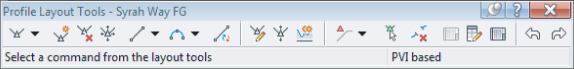
Figure 7.15 Profile Layout Tools toolbar

![]()
![]()
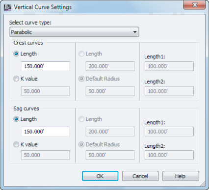
Figure 7.16 The Vertical Curve Settings dialog
![]()
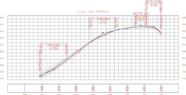
Figure 7.17 A completed layout profile with labels
When this exercise is complete, you may close the drawing. A finished copy of this drawing is available from the book's web page with the filename LayoutByPVI_FINISHED.dwg or LayoutByPVI_METRIC_FINISHED.dwg.
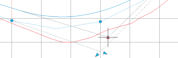
The layout profile is labeled with the Complete Label Set you selected in the Create Profile dialog. As you'd expect, this labeling and the layout profile are dynamic. If you select the profile and then zoom in on this profile line, not the labels or the profile view, you'll see something like Figure 7.18.
Figure 7.18 The types of grips on a layout profile
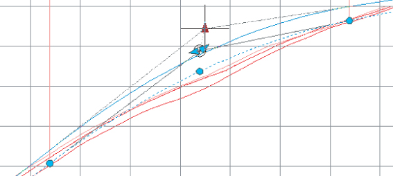
The PVI-based layout profiles include the following unique grips:
Vertical Triangular Grip
The vertical triangular grip at the PVI point is the PVI grip. Moving this alters the inbound and outbound tangents, but the curve remains in place with the same design parameters of length and type.
Angled Triangular Grips
The angled triangular grips on either side of the PVI are sliding PVI grips. Selecting and moving either moves the PVI, but movement is limited to along the tangent of the selected grip. The curve length isn't affected by moving these grips, but the PVI station and elevation will be, as well as the grade of the other tangent.
Circular Pass-Through Grips
The circular pass-through grips near the PVI and at each end of the curve are curve grips. Moving any of these grips makes the curve longer or shorter without adjusting the inbound or outbound tangents or the PVI point.
Although this simple pick-and-go methodology works for preliminary layout, it lacks a certain amount of control typically required for final design. For that, you'll use another method of creating PVIs:
Figure 7.19 The Transparent Commands toolbar
![]()
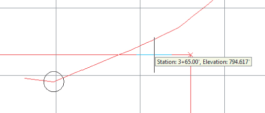
Figure 7.20 A jig appears when you use the Profile Station Elevation transparent command
![]()
![]()
Figure 7.21 Using the Transparent Commands toolbar to create a layout profile
When this exercise is complete, you may close the drawing. A finished copy of this drawing is available from the book's web page with the filename LayoutByPVITransparent_FINISHED.dwg or LayoutByPVITransparent_METRIC_FINISHED.dwg.
Using PVIs to define tangents and fitting curves between them is the most common approach to create a layout profile, but you'll look at an entity-based design in the next section.
Layout by Entity
Working with the concepts of fixed, floating, and free entities as you did with alignments in Chapter 6, you'll lay out a design profile in this exercise:
![]()
![]()
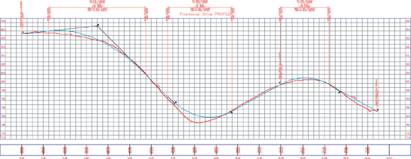
Figure 7.22 Some tangent and vertical curve entities placed on Frontenac Drive
![]()
![]()
![]()
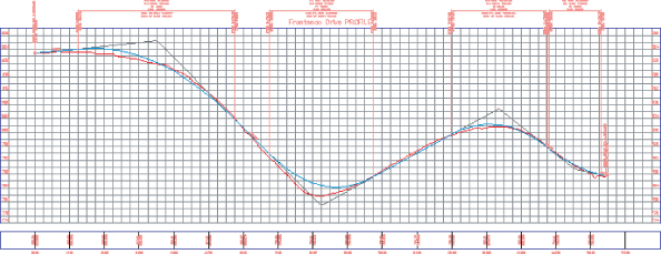
Figure 7.23 Completed profile built using entities
When this exercise is complete, you may close the drawing. A finished copy of this drawing is available from the book's web page with the filename LayoutByEntity_FINISHED.dwg or LayoutByEntity_METRIC_FINISHED.dwg.
With the entity-creation method, grip editing works in a similar way to other layout methods based on the fixed, floating, and free constraints.
Profile Layout Tools
![]()
Although we have touched on many of the available tools in the Profile Layout Tools toolbar, as shown in Figure 7.24, there are still many that we have not.
Figure 7.24 Profile Layout Tools toolbar
Draw Tangent Drop-Down
The Draw Tangent drop-down button contains three options: Draw Tangents, Draw Tangents With Curves, and Curve Settings. Draw Tangents lays out a profile point to point with no curves. Draw Tangent With Curves lays out a profile from point to point with the curve type and length determined from the Curve Settings. Curve Settings sets the type of curve (parabolic, circular, asymmetric), default crest and sag K values, and default crest and sag lengths.
Insert PVI
The Insert PVI button adds a new PVI at the specified location, consequently breaking an existing tangent and generating two new tangents connected to the new PVI.
Delete PVI
The Delete PVI button removes an existing PVI at the specified location, consequently taking two tangents and replacing them with a single tangent.
Move PVI
The Move PVI button allows you to select an existing PVI and relocate it to a specified location while keeping the two existing tangents. You can get the same result by grip-editing the PVI with the vertical triangular grip, as described earlier.
Tangent Creation Drop-Down
The Tangent Creation Drop-down button contains six tools:
- Fixed Tangent (Two Points)
- Fixed Tangent – Best Fit
- Float Tangent (Through Point)
- Float Tangent – Best Fit
- Free Tangent
- Solve Tangent Intersection
Vertical Curve Creation Drop-Down
The Vertical Curve Creation Drop-down button contains 14 options:
- Fixed Vertical Curve (Three Points)
- Fixed Vertical Curve (Two Points, Parameter)
- Fixed Vertical Curve (Entity End, Through Point)
- Fixed Vertical Curve (Two Points, Grade At Start Point)
- Fixed Vertical Curve (Two Points, Grade At End Point)
- Fixed Vertical Curve – Best Fit
- Floating Vertical Curve (Parameter, Through Point)
- Floating Vertical Curve (Through Point, Grade)
- Floating Vertical Curve – Best Fit
- Free Vertical Curve (Parameter)
- Free Vertical Parabola (PVI Based)
- Free Asymmetrical Parabola (PVI Based)
- Free Circular Curve (PVI Based)
- Free Vertical Curve – Best Fit
Convert AutoCAD Line And Spline
The Convert AutoCAD Line And Spline button takes a singular line/spline and converts it into a profile object, either a tangent or a three-point vertical curve as applicable.
Insert PVIs – Tabular
The Insert PVIs – Tabular button allows you to enter PVI station and elevation information in a table-like dialog, which is helpful if you want to create multiple PVIs at once using station and elevation information. This table allows you to insert PVIs and curves anywhere geometrically possible in the profile. The order in which you insert the PVIs isn't important either when using this method of entry.
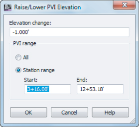
Raise/Lower PVIs
The Raise/Lower PVIs button allows you to raise or lower a profile at a specified distance for either the entire profile or for the PVIs within a specified station range. This button will be discussed in a later exercise on Other Profile Edits.
Copy Profile
The Copy Profile button allows you to copy either the entire profile or within a specified station range. This button will be discussed in a later exercise in the “Other Profile Edits” section.
PVI or Entity Based Drop-Down
The PVI or Entity Based drop-down button allows you to choose to select and display profile layout parameters based on either PVI or Entity.
Select PVI or Select Entity
The Select PVI or Select Entity button opens the Profile Layout Parameters dialog for the selected PVI or Entity.
Delete Entity
The Delete Entity button removes a selected curve or tangent.
Edit Best Fit Data For All Entities
The Edit Best Fit Data For All Entities button turns on the display of a table of the regression data for a profile that was created by best fit. A discussion of Best Fit Profile is provided in the next section.
Profile Layout Parameters
The Profile Layout Parameters button opens the Profile Layout Parameters dialog, which shows numeric data for editing the selected entity or PVI.
Profile Grid View
The Profile Grid View button opens the Profile Entities tab in Panorama, showing information about all the entities and PVIs in the profile. This is where you have access to make edits on all the entities of the profile.
Undo/Redo
The Undo and Redo buttons reverse the last command or the last undo operation.
The Best Fit Profile
You've surveyed along a centerline, and you need to closely approximate the tangents and vertical curves as they were originally designed and constructed.
![]()
The Create Best Fit Profile option is found in the Home tab ⇒ Create Design panel, on the Profile drop-down. Once you select a profile view, the Create Best Fit Profile dialog appears, as shown in Figure 7.25.
Figure 7.25 Create Best Fit Profile dialog
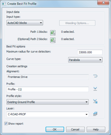
Similar to the best fit alignment we discussed in Chapter 6, a best fit profile can be based on an Input Type setting of AutoCAD Blocks, AutoCAD 3D Polylines, AutoCAD Points, COGO Points, Surface Profile, or Feature Lines. The most common option is Surface Profile.
The command attempts to run a complex algorithm to determine the best fit profile, including both tangents and vertical curves. However, the only best fit option available for determining vertical curves is the maximum curve radius. The maximum curve radius is a formula rarely used in the design of parabolic curves, the most common curves found in roadway design. Once the analysis is run, a Best Fit Report is provided; however, unlike the Best Fit command for lines and curves as seen in Chapter 1, “The Basics,” this command has no options for selecting or deselecting points, making the command somewhat cumbersome.
In some cases, the commands you choose to use in a given scenario, as promising as the name may sound, may actually prove to be more of a hindrance than a help. The Best Fit Profile command may be one of these cases. The command attempts to perform an analysis on all the sampled existing ground profile points in a profile view, the options are limited, and in the end, you may find a good pair of eyes and graphical analysis using other profile creation methods are less time consuming and produce an equally valid result.
It is important to understand all the commands at your disposal, but you are not required to use each one in a production environment. If results don't meet your needs and you've spent considerable time with a single method, find another method, or methods, that accomplish the same task. Remember, at the end of the day, you still have sheets to cut and plans to get out the door. You're limited only by your selection of commands and your creativity.
Creating a Profile from a File
Working with profile information in the AutoCAD Civil 3D environment is nice, but it isn't the only place where you can create or manipulate this sort of information. Many programs or analysis packages generate profile information. One common case is the plotting of a hydraulic grade line against a stormwater network profile of the pipes. When information comes from outside the program, it is often output in myriad formats. If you convert this format to the format required by AutoCAD Civil 3D, the profile information can be input directly.
There is a specific format that is required for creating a profile from a text file. Each line is a PVI definition (station and elevation) listed in ascending order. The station should not include the plus character (use 100, not 1+00 or 0+100). Curve information is an optional third bit of data on any line except for the first and last lines in the file. The vertical curve that is created will be a parabolic curve, which is the most popular type of vertical curve. Note that each line is space delimited. Here's one example of a profile text file:
0 550.76
127.5 552.24
200.8 554 100
256.8 557.78 50
310.75 561
In this example, the third and fourth lines include the curve length as the optional third piece of information. The only inconvenience of using this input method is that the information in Civil 3D doesn't directly reference the text file. Once the profile data is imported, no dynamic relationship exists with the text file, but other methods can be used to edit the profile once imported.
In this exercise, you'll import a small text file to see how the function works:

Figure 7.26 Completed profile created from a file
When this exercise is complete, you may close the drawing. A finished copy of this drawing is available from the book's web page with the filename ProfileFromFile_FINISHED.dwg or ProfileFromFile_METRIC_FINISHED.dwg.
Now that you've tried the three main ways of creating profile information, you'll edit a profile in the next section.
Editing Profiles
The methods just reviewed let you quickly create profiles. You saw how sampled profiles reflect changes in the parent alignment and how to lay out a design profile using a few different methodologies. You also imported a text file with profile information. In all these cases, you just left the profile as originally designed with no analysis or editing.
This section will begin to look at some of the profile editing methods available. The most basic is a more precise grip-editing methodology, which you'll learn about first. Then you'll see how to modify the PVI-based layout profile, how to change out the components that make up a layout profile, and how to use some other miscellaneous editing functions.
Grip Profile Editing
Once a profile layout is in place, sometimes a simple grip edit will suffice. But for precision editing, you can use a combination of the grips and the buttons on the Transparent Commands toolbar, as in this short exercise:
Figure 7.27 Grip-editing a PVI
![]()
When this exercise is complete, you may close the drawing. A finished copy of this drawing is available from the book's web page with the filename GripEditingProfiles_FINISHED.dwg or GripEditingProfiles_METRIC_FINISHED.dwg.
The grips can go from quick-and-dirty editing tools to precise editing tools when you use them in conjunction with the transparent commands in the profile view. They lack the ability to precisely control a curve length, though, so you'll look at editing a curve next.
Parameter and Panorama Profile Editing
Beyond the simple grip edits, but before changing out the components of a typical profile, you can modify the values that generate an individual component. In this exercise, you'll use the Profile Layout Parameter dialog and the Panorama to modify the curve properties on your design profile:
![]()
![]()
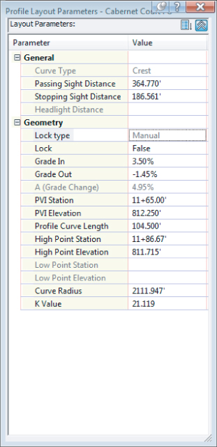
Figure 7.28 The Profile Layout Parameters dialog
![]()
Figure 7.29 Direct editing of the curve length in Panorama

Figure 7.30 The completed editing of the curve length in the layout profile
When this exercise is complete, you may close the drawing. A finished copy of this drawing is available from the book's web page with the filename ParameterEditingProfiles_FINISHED.dwg or ParameterEditingProfiles_METRIC_FINISHED.dwg.
You can use these tools to modify the PVI points or tangent parameters, but they won't let you add or remove an entire component. You'll do that in the next section.
Component-Level Editing
In addition to editing basic parameters and locations, sometimes you have to add or remove entire components. In this exercise, you'll delete a PVI, remove a curve from an area in order to revise a nearby PVI location, and insert a new curve into the layout profile:
![]()
![]()
![]()
Figure 7.31 The completed editing of the curve using component-level editing

When this exercise is complete, you may close the drawing. A finished copy of this drawing is available from the book's web page with the filename ComponentEditingProfiles_FINISHED.dwg or ComponentEditingProfiles_METRIC_FINISHED.dwg.
Editing profiles using any of these methods gives you precise control over the creation and layout of your vertical design. In addition to these tools, some of the tools on the Profile Layout Tools toolbar are worth investigating and somewhat defy these categories. You'll look at them next.
Other Profile Edits
Some handy tools exist on the Profile Layout Tools toolbar for performing specific actions. These tools aren't normally used during the preliminary design stage, but they come into play as you're working to create a final design for grading or corridor design. They include raising or lowering a whole layout in one shot, as well as copying profiles. Try this exercise:
![]()
Figure 7.32 The Copy Profile Data dialog

![]()
Figure 7.33 The Raise/Lower PVI Elevation dialog
When this exercise is complete, you may close the drawing. A finished copy of this drawing is available from the book's web page with the filename OtherProfileEdits_FINISHED.dwg or OtherProfileEdits_METRIC_FINISHED.dwg.
Generating a copy is useful if you want to remember a conceptual profile layout but would like to experiment with a different layout. The copies do not stay dynamically related to one another.
Using the layout and editing tools discussed in these sections, you should be able to design and draw any combination of profile information presented to you.
Matching Profile Elevations at Intersections
Up to now, you have learned how to use some of the available tools for modifying profiles, but you might be wondering about the intersecting roads and how the profiles will interact with one another. Have no fear; we are going to discuss those later in Chapter 10 when we discuss corridor intersections.
Profile Views
![]()
Working with vertical data is an integral part of building the model. Once profile information has been created in any number of ways, displaying it to make sense is another task. It can't be stated enough that profiles and profile views are not the same thing. The profile view displays the profile data. A single profile can be shown in an infinite number of views, with different grids, exaggeration factors, labels, or linetypes. In this section, you'll look at the various methods available for creating profile views.
Creating Profile Views during Sampling
The easiest way to create a profile view is to draw it as an extended part of the surface sampling procedure as shown in the first exercise. By combining the profile sampling step with the creation of the profile view, you have avoided one more trip to the menus. This is the most common method of creating a profile view, but we'll look at a manual creation in the next section.
Creating Profile Views Manually
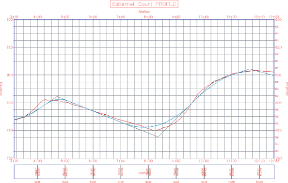
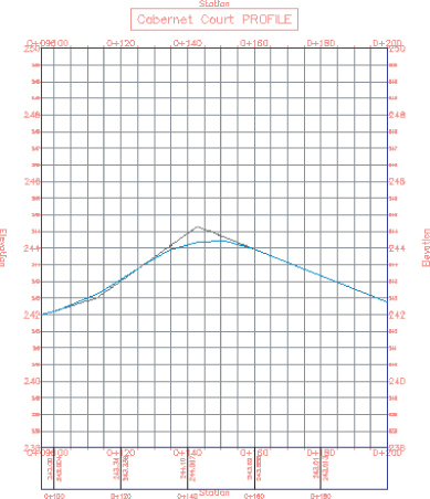
Once an alignment has profile information associated with it, any number of profile views might be needed to display the proper information in the right format. To create a second, third, or even tenth profile view once the sampling is done, you must use a manual creation method. In this exercise, you'll create a profile view manually for an alignment that already has a surface-sampled profile associated with it:

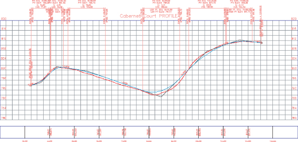
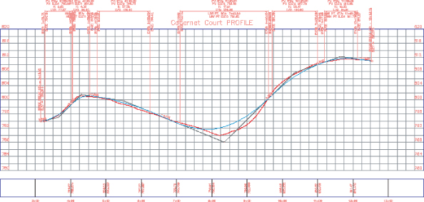
Figure 7.34 The completed profile view of Cabernet Court using the Full Grid profile view style
When this exercise is complete, you may close the drawing. A finished copy of this drawing is available from the book's web page with the filename ProfileViews_FINISHED.dwg or ProfileViews_METRIC_FINISHED.dwg.
Using these two creation methods, you've made short, simple profile views, but in the next exercise we will look at a longer alignment, as well as some more of the options available in the Create Profile View wizard.
Splitting Views
Dividing up the data shown in a profile view can be time consuming. The Profile View wizard is used for simple profile view creation, but the wizard can also be used to create manually limited profile views, staggered (or stepped) profile views, multiple profile views with gaps between the views, and stacked profiles (aka three-line profiles). You'll look at these variations on profile view creation in this section.
Creating Manually Limited Profile Views
Continuous profile views like you made in the exercises prior to this point work well for design purposes, but they are often unusable for plotting or exhibiting purposes. In this exercise, you'll use the Profile View wizard to create a manually limited profile view. This variation will allow you to control how long and how high each profile view will be, thereby making the views easier to plot.
Figure 7.35 The start and end stations for the user-specified profile view

Figure 7.36 Applying user-specified station and height values to a profile view

Creating Staggered Profile Views
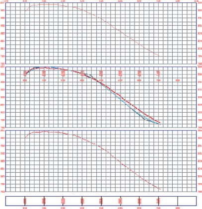
When large variations occur in profile height, the profile view must often be split just to keep from wasting much of the page with empty grid lines. In this exercise, you use the Profile View wizard to create a staggered, or stepped, view:
Figure 7.37 Split Profile View settings

Figure 7.38 A staggered (stepped) split profile view created via the wizard
The profile view is split into views according to the settings that were selected in the Create Profile View wizard in step 6. The first portion of the profile view shows the profile from 0 to the station where the elevation change of the profile exceeds the limit for height. The next portion of the profile view displays the same, and so on for the rest of the profile. Each of these portions is part of the same profile view and can be adjusted via the Profile View Properties dialog.
When this exercise is complete, you may save and keep the drawing open to continue on to the next exercise. If you would like to view the result of this exercise, it is included in the finished drawing (along with the finished portions of the previous exercise and next exercise) available from the book's web page (ProfileViewsSplit_FINISHED.dwg or ProfileViewsSplit_METRIC_FINISHED.dwg).
Creating Gapped Profile Views
Profile views must often be limited in length and height to fit a given sheet size. Gapped views are a way to show the entire length and height of the profile, by breaking the profile into different sections with “gaps” or spaces between each view.
When you are using the Plan and Production tools (covered in Chapter 17, “Plan Production”), the gapped profile views are automatically created.
In this exercise, you will use a variation of the Create Profile View wizard called the Create Multiple Profile Views wizard to create gapped views automatically:
![]()
Figure 7.39 The Create Multiple Profile Views – General wizard page
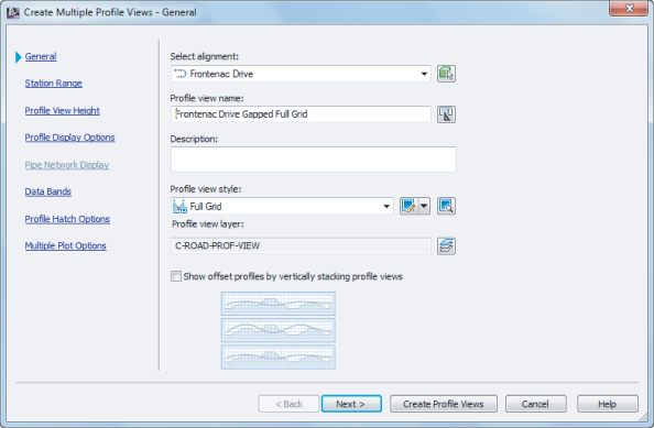
Figure 7.40 The Create Multiple Profile Views – Multiple Plot Options wizard page

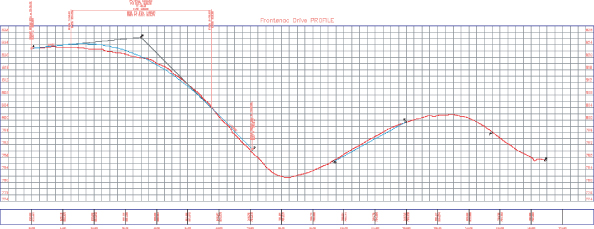
Figure 7.41 The staggered and gapped profile views of the Frontenac alignment
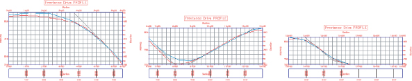
The gapped profile views are the three profile views on the bottom of the screen and, just like the staggered profile view, show the entire alignment from start to finish. Unlike the staggered view, however, the gapped view is separated by a “gap” into three profile views. In addition, the gapped profile views are independent of each other so they can be modified to have their own styles, properties, and labeling associated with them, making them useful when you don't want a view to show information that is not needed on a particular section. This is also the primary way to create divided profile views for sheet production.
When this exercise is complete, you may close the drawing. A finished copy of this drawing showing the results of the previous three exercises is available from the book's web page with the filename ProfileViewsSplit_FINISHED.dwg or ProfileViewsSplit_METRIC_FINISHED.dwg.
Creating Stacked Profile Views
In some parts of the United States, a three-line profile view is a common requirement. In this situation, the centerline is displayed in a central profile view, with left and right offsets shown in profile views above and below the centerline profile view. These are then typically used to show top-of-curb design profiles in addition to the centerline design. In this exercise, you look at how the Create Profile View wizard makes generating these stacked views a simple process:
Figure 7.42 The Create Profile View – Stacked Profile wizard page

Figure 7.43 Setting the stacked view options for each view

Figure 7.44 Completed stacked profiles
When this exercise is complete, you may close the drawing. A finished copy of this drawing is available from the book's web page with the filename StackedProfiles_FINISHED.dwg or StackedProfiles_METRIC_FINISHED.dwg.
Like the gapped profile views that you generated in a previous exercise, the profile views are independent of one another so they can be modified to have their own styles, properties, and labeling associated with them. The stacking here simply automates a process that many users previously found tedious. At this point you do not have finished grade information at the offsets, but you can add it to these views later by editing the Profile View Properties for those profile views.
When you create a profile, the profile will automatically be visible in all profile views based on that same alignment by default. In the Profile View Properties dialog, you can always turn the Draw option off for any profile that you don't want visible in a profile view.
Editing Profile Views
Once profile views have been created, things get interesting. Any number of modifications to the view itself can be applied, even before editing the styles, which makes profile views one of the most flexible objects of the AutoCAD Civil 3D package. In this series of exercises, you'll look at a number of changes that can be applied to any profile view in place.
Profile View Properties
Picking a profile view from the Profile View contextual tab ⇒ Modify View panel and choosing Profile View Properties yields the dialog shown in Figure 7.45. The properties of a profile include the style applied, station and elevation limits, the number of profiles displayed, and the bands associated with the profile view. If a pipe network is displayed, a tab labeled Pipe Networks will appear. These tabs should look very similar to the links in the sidebar of the Create Profile View wizard.
Figure 7.45 Typical Profile View Properties dialog
Adjusting the Profile View Station Limits
In spite of the wizard, there are often times when a profile view needs to be manually adjusted. For example, the most common change is to limit the length of the profile view that is being shown so it fits on a specific size of paper or viewport. You can make some of these changes during the initial creation of a profile view (as shown in a previous exercise), but you can also make changes after the profile view has been created.
One way to do this is to use the Profile View Properties dialog to make changes to the profile view. The profile view is an AutoCAD Civil 3D object, so it has properties and styles that can be adjusted in this dialog to make the profile view look like you need it to.
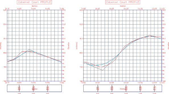
Figure 7.46 Adjusting the end station values for Cabernet Court
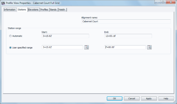
Figure 7.47 A manually created gap between profile views
When this exercise is complete, you may save and keep the drawing open to continue on to the next exercise. If you would like to view the result of this exercise, it is included in the finished drawing (along with the finished portions of the next two exercises) available from the book's web page (ProfileViewProperties_FINISHED.dwg or ProfileViewProperties_METRIC_FINISHED.dwg).
In addition to creating gapped profile views by changing the profile properties, you could show phase limits by applying a different style to the profile in the second view.
Adjusting the Profile View Elevations
Another common issue is the need to control the height of the profile view. Civil 3D automatically sets the datum and the top elevation of profile views on the basis of the data to be displayed. In most cases this is adequate, but in others, this simply creates a view too large for the space allocated on the sheet or does not provide the adequate room for layout PVIs to be laid out.
Figure 7.48 Modifying the height of the profile view
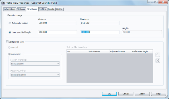
Figure 7.49 The updated profile view with the heights manually adjusted
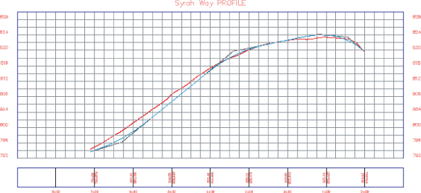
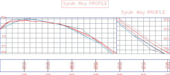
Figure 7.50 Defining a Split Profile View on the Elevations tab
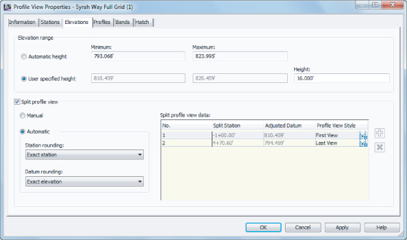
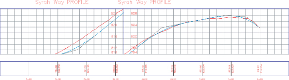
Figure 7.51 A split profile view for the Syrah Way alignment
When this exercise is complete, you may save and keep the drawing open to continue on to the next exercise. If you would like to view the result of this exercise, it is included in the finished drawing (along with the finished portions of the previous exercise and next exercise) available from the book's web page (ProfileViewProperties_FINISHED.dwg or ProfileViewProperties_METRIC_FINISHED.dwg).
Automatically creating split views is a good starting point, but you'll often have to tweak them as you've done here. The selection of the proper profile view styles is an important part of the Split Profile View process. We'll look at object styles in Chapter 21.
Profile Display Options
AutoCAD Civil 3D allows the creation of literally hundreds of profiles for any given alignment. Doing so makes it easy to evaluate multiple design solutions, but it can also mean that profile views get very crowded. In this exercise, you'll look at some profile display options that allow the toggling of various profiles within a profile view:
Figure 7.52 The Cabernet Court profile view with the Draw option toggled off for the EG profile
Toggling off the Draw option for the EG surface has created a profile view style in which a profile of the existing ground surface will not be drawn on the profile view.
The sampled profile from the EG surface still exists under the Cabernet Court alignment; it simply isn't shown in the current profile view.
When this exercise is complete, you may close the drawing. A finished copy of this drawing showing the results of the previous three exercises is available from the book's web page with the filename ProfileViewProperties_FINISHED.dwg or ProfileViewProperties_METRIC_FINISHED.dwg.
Now that you've modified a number of styles, let's look at another option that is available on the Profile View Properties dialog: bands.
Profile View Bands
Data bands are horizontal elements that display additional graphical and numerical information about the profile or alignment that is referenced in a profile view. Bands can be applied to both the top and bottom of a profile view, and there are six different band types:
Profile Data Bands
Display information about the selected profile. This information can include simple elements such as elevation, or more complicated information such as the cut-fill between two profiles at the given station.
Vertical Geometry Bands
Create an iconic view of the elements making up a profile. Typically used in reference to a design profile, vertical data bands make it easy for a designer to see where vertical curves are information about the tangents and vertical curves located along the alignment.
Horizontal Geometry Bands
Create a simplified view of the horizontal alignment elements, giving the designer or reviewer information about line, curve, and spiral segments and their relative location to the profile data being displayed.
Superelevation Bands
Display the various options for Superelevation values at the critical points along the alignment.
Sectional Data Bands
Can display information about the sample line locations, the distance between them, and other sectional-related information.
Pipe Data Bands
Can display specific information such as part, offset, elevation, or direction about each pipe or structure being shown in the profile view.
In this exercise, you'll add bands to give feedback on the EG and layout profiles, as well as horizontal and vertical geometry:
Figure 7.53 The Bands tab of the Profile View Properties dialog
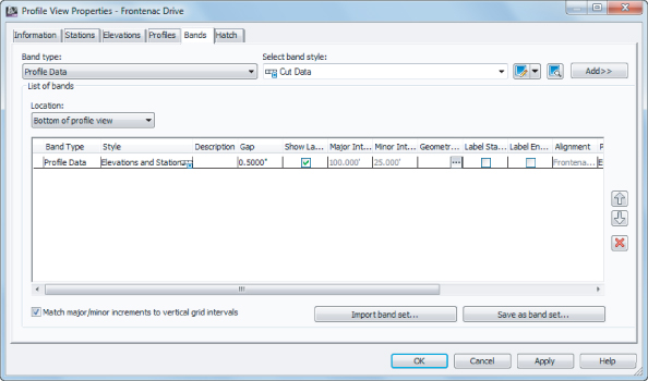
Figure 7.54 The Geometry Points To Label In Band dialog showing the Alignment Points tab (left) and the Profile Points tab (right)
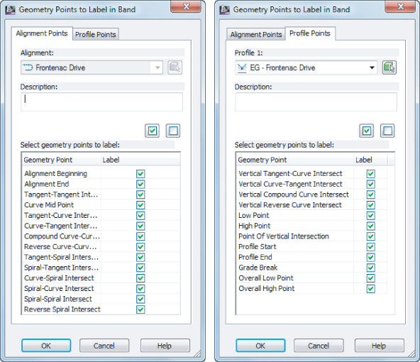
Figure 7.55 Applying bands to a profile view

Figure 7.56 Setting the profile view bands to reference the Frontenac Drive FG profile

Figure 7.57 Completed profile view with the Bands set appropriately
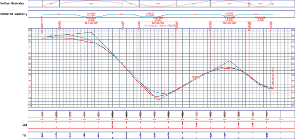
When this exercise is complete, you may close the drawing. A finished copy of this drawing is available from the book's web page with the filename ProfileViewBands_FINISHED.dwg or ProfileViewBands_METRIC_FINISHED.dwg.
Bands use the Profile1 and Profile2 designation as part of their style construction. By changing the profile referenced as Profile1 or Profile2, you change the values that are calculated and displayed (e.g., existing versus proposed elevations). These bands are just more items that are driven by object styles, which you will learn more about in Chapter 21.
We will look at using Band Sets a little later in this chapter.
Profile View Hatch
Sometimes it is necessary to shade cut/fill areas in a profile view. The settings on the Hatch tab of the Profile View Properties dialog are used to specify upper and lower cut/fill boundary limits for associated profiles (see Figure 7.58). Shape styles from the General Multipurpose Styles collection found on the Settings tab of Toolspace can also be selected here. These settings include the following:
Figure 7.58 Shape style selection on the Hatch tab of the Profile View Properties dialog

Cut Area
Click this button to add hatching to a profile view in areas of the cut (the layout profile is at a lower elevation than the sampled surface profile).
Fill Area
Click this button to add hatching to a profile view in areas of the fill (the layout profile is at a higher elevation than the sampled surface profile).
Multiple Boundaries
Click this button to add hatching to a profile view in areas of a cut/fill where the area must be averaged between two existing profiles (for example, finished ground at the centerline vs. the left and right top of a curb).
From Criteria
Click this button to add hatch in areas where quantity takeoff criteria are used to define a hatch region.
Figure 7.59 shows a cut and fill hatched profile based on the criteria shown previously in Figure 7.58.
Figure 7.59 A portion of the Frontenac Drive Profile shown with cut and fill shading

Mastering Profiles and Profile Views
One of the most difficult concepts to master in AutoCAD Civil 3D is the notion of which settings control which display property. Although the following two rules may sound overly simplistic, they are easily forgotten in times of frustration:
- Every object has a label and an object style.
- Every label has a label style.
Furthermore, if you can remember that there is a distinct difference between a profile object and the profile view object you place it in, you'll be well on your way to mastering profiles and profile views. When in doubt, select an object, right-click, and pay attention to the Civil 3D commands available. Label styles and object styles will be discussed further in Chapters 20 and 21, respectively.
Profile View Labeling Styles
Now that the profile view is created, the profile view grid spacing is set, and the titles all look good, it's time to add some specific callouts and detail information. Civil 3D uses profile view labels and bands for annotating. The specific label styles will be discussed further in Chapter 20, but for now we will just discuss how to apply the labels.
View Annotation
Profile view annotations label individual points in a profile view, but they are not tied to a specific profile object. Profile view labels can be station elevation, depth labels, or projection labels. Station elevation labels can be used to label a single point or the depth between two points in a profile while recognizing the vertical exaggeration of the profile view and applying the scaling factor to label the correct depth. In this exercise, you'll use both the station elevation label and the depth label:
Figure 7.60 An elevation label for a profile station
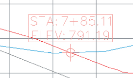
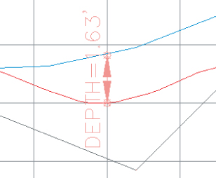
Figure 7.61 A depth label applied to the Cabernet Court profile view
When this exercise is complete, you may close the drawing. A finished copy of this drawing is available from the book's web page with the filename ProfileViewLabels_FINISHED.dwg or ProfileViewLabels_METRIC_FINISHED.dwg.
Depth labels can be handy in earthworks situations where cut and fill become critical, and individual spot labels are important to understanding points of interest, but most design documentation is accomplished with labels placed along the profile view axes in the form of data bands. The next section describes these band sets.
Band Sets
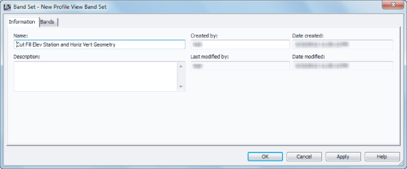
Band sets are simply collections of bands, much like the profile label sets or alignment label sets. In this exercise, you'll save a band set and then apply it to a second profile view:
Figure 7.62 The Information tab for the Band Set – New Profile View Band Set dialog
Your Syrah Way profile view (Figure 7.63) now looks like the Frontenac Drive profile view.
Figure 7.63 Completed profile view after importing the band set and matching properties

Band sets allow you to create uniform labeling and callout information across a variety of profile views. By using a band set, you can apply myriad settings and styles that you've assigned to a single profile view to a number of profile views. The simplicity of enforcing standard profile view labels and styles makes using profiles and profile views simpler than ever.
When this exercise is complete, you may close the drawing. A finished copy of this drawing is available from the book's web page with the filename ProfileViewBandSets_FINISHED.dwg or ProfileViewBandSets_METRIC_FINISHED.dwg.
Profile Labels
It's important to remember that the profile and the profile view aren't the same thing. The labels discussed in this section are those that relate directly to the profile but are visible for a specific profile view. This usually means station-based labels, individual tangent and curve labels, or grade breaks.
Applying Labels
As with alignments, you can apply labels as a group of objects separate from the profile. In this portion of the exercise, you'll learn how to add labels along a profile object:
![]()
Figure 7.64 An empty Profile Labels dialog
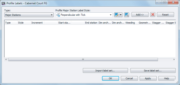
Figure 7.65 The Geometry Points dialog appears when you apply labels to horizontal geometry points.

Figure 7.66 Labels applied to major stations and alignment geometry points
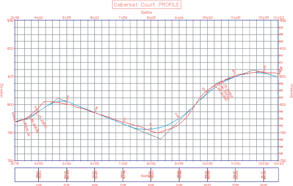
Figure 7.67 Modifying the major station labeling increment

When this exercise is complete, you may close the drawing. A finished copy of this drawing is available from the book's web page with the filename ApplyingProfileLabels_FINISHED.dwg or ApplyingProfileLabels_METRIC_FINISHED.dwg.
As you can see, applying labels one at a time could turn into a tedious task. After you learn about the types of labels available, you may want to revisit this dialog and use the Import Label Set and Save Label Set buttons, which work similarly to the Import Band Set and Save Band Set buttons that we discussed previously. A further discussion, including more of the profile labels that are available, is provided in Chapters 20 and 21.
Profile Label Sets
Applying labels to both crest and sag curves, tangents, grade breaks, and geometry with the label style selection and various options can be monotonous. Thankfully, Civil 3D gives you the ability to use label sets, as in alignments, to make the process quick and easy. Just as you saved and imported band sets in a previous example, you can save and import label sets as well.
In all of the previous examples you used either the Complete Label Set or the _No Labels label set, which you specified on the Profile Display Options wizard page.
Label sets are the best way to apply profile labeling uniformly. When you're working with a well-developed set of styles and label sets, it's quick and easy to go from sketched profile layout to plan-ready output. We will discuss profile label sets in further detail and go over an example in Chapter 20.
Profile Utilities
One common requirement is to compare profile data for objects that are aligned similarly but not parallel. Another is the ability to project objects from a plan view into a profile view. The abilities to superimpose profiles and project objects are both discussed in this section.
Superimposing Profiles
In a profile view, a profile is sometimes superimposed to show one profile adjacent to another (e.g., a ditch adjacent to a road centerline). In this brief exercise, you'll superimpose one of your street designs onto the other to see how they compare over a certain portion of their length:
![]()
Figure 7.68 The Superimpose Profile Options dialog
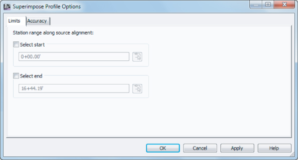
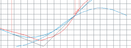
Figure 7.69 The Frontenac Drive layout profile superimposed on the Cabernet Court profile view
When this exercise is complete, you may close the drawing. A finished copy of this drawing is available from the book's web page with the filename SuperimposeProfiles_FINISHED.dwg or SuperimposeProfiles_METRIC_FINISHED.dwg.
Note that the vertical curve in the Frontenac Drive layout profile has been approximated on the Cabernet Court profile view, using a series of PVIs. Superimposing works by projecting a line from the target alignment (Cabernet Court) to a perpendicular intersection with the other source alignment (Frontenac Drive).
The target alignment is queried for an elevation at the intersecting station and a PVI is added to the superimposed profile. Note that this superimposed profile is still dynamic! A change in the Frontenac Drive layout profile will be reflected on the Cabernet Court profile view.
Object Projection
Some AutoCAD and some AutoCAD Civil 3D objects can be projected from a plan view into a profile view. The list of available AutoCAD objects includes points, blocks, 3D solids, and 3D polylines. The list of available AutoCAD Civil 3D objects includes COGO points, feature lines, and survey figures. These objects can be projected to the objects elevation, a manually selected elevation, a surface, or a profile. In the following exercise, you'll project a 3D object into a profile view:
![]()
Figure 7.70 A completed Project Objects To Profile View dialog
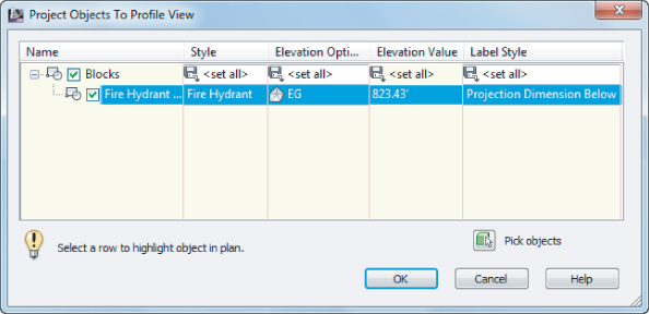
Figure 7.71 The COGO point object projected into a profile view

![]()
Figure 7.72 Select the Syrah Way FG elevation

Figure 7.73 The COGO point object projected onto the Syrah Way FG profile
When this exercise is complete, you may close the drawing. A finished copy of this drawing is available from the book's web page with the filename ObjectProjection_FINISHED.dwg or ObjectProjection_METRIC_FINISHED.dwg.
Once an object has been projected into a profile view, the Profile View Properties dialog will display a new Projections tab. Projected objects will remain dynamically linked with respect to their plan placement. If you move them manually after placing them dynamically, a warning will appear to confirm that you want to break the dynamic setting. Because profile views and section views are similar in nature, objects can be projected into section views in the same fashion. However, projecting a feature line onto a profile view will give you a different result than projecting it onto a section view. On a profile view, it looks more like a superimposed profile. On a section view, it's more like a pipe crossing since it only appears where it intersects the section line.
Quick Profile
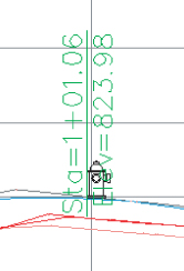
There are going to be times when all you want is to quickly look at a profile and not keep it for later use. When this is the case, instead of creating an alignment, a profile, and a profile view, you can instead create a quick profile. A quick profile is a temporary object that will not be saved with the drawing. You can create a quick profile for 2D or 3D lines or polylines, lot lines, feature lines, survey figures, or even a series of points.
From the Home tab ⇒ Create Design panel, choose Profile ⇒ Quick Profile. The command line will state Select object or [by Points]:. Once you select your object (or points), the Create Quick Profiles dialog is displayed, as shown in Figure 7.74.
Figure 7.74 The Create Quick Profiles dialog
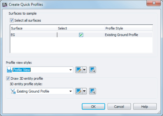
You can select which surface you want to sample as well as what profile view style and 3D entity profile style to use.
The Bottom Line
Sample a surface profile with offset samples.
Using surface data to create dynamic sampled profiles is an important advantage of working with a three-dimensional model. Quick viewing of various surface centerlines and grip-editing alignments makes for an effective preliminary planning tool. Combined with offset data to meet review agency requirements, profiles are robust design tools in Civil 3D.
Master It
Open the MasteringProfiles.dwg file (or MasteringProfiles_METRIC.dwg file) and sample the ground surface along Alignment A, along with offset values at 15′ left and 15′ right (or 4.5 m left and 4.5 m right) of the alignment. Generate a profile view showing this information using the Major Grids profile view style with no data band sets.
Lay out a design profile on the basis of a table of data.
Many programs and designers work by creating pairs of station and elevation data. The tools built into Civil 3D let you input this data precisely and quickly.
Master It
In the MasteringProfiles.dwg file (or the MasteringProfiles_METRIC.dwg file), create a layout profile on Alignment A using the Layout profile style and a Complete Label Set with the following information for Imperial users:
| Station | PVI Elevation | Curve Length |
| 0+00 | 822.00 | |
| 1+80 | 825.60 | 300′ |
| 6+50 | 800.80 |
| Station | PVI Elevation | Curve Length |
| 0+000 | 250.400 | |
| 0+062 | 251.640 | 100 m |
| 0+250 | 244.840 |
Add and modify individual entities in a design profile.
The ability to delete, modify, and edit the individual components of a design profile while maintaining the relationships is an important concept in the 3D modeling world. Tweaking the design allows you to pursue a better solution, not just a working solution.
Master It
In the MasteringProfiles.dwg file (or the MasteringProfiles_METRIC.dwg file) used in the previous exercise, on profile A modify the original curve so that it is 200′ (or 60 m for metric users). Then insert a PVI at Station 4+90, Elevation 794.60 (or at Station 0+150, Elevation 242.840 for metric users) and add a 300′ (or 96 m for metric users) parabolic vertical curve at the newly created PVI.
Apply a standard band set.
Standardization of appearance is one of the major benefits of using styles in labeling. By applying band sets, you can quickly create plot-ready profile views that have the required information for review.
Master It
In the MasteringProfiles.dwg (or the MasteringProfiles_METRIC.dwg) file, apply the Cut and Fill band set to the layout profile created in the previous exercise with the appropriate profiles referenced in each of the bands.