Chapter 15
Storm and Sanitary Analysis
One of the trickiest and most controversial parts of a civil designer's job is determining where water and wastewater will go in a site. Civil 3D offers a variety of tools for designing and analyzing the hydraulic and hydrology portions of your project. Hydraulic calculations for pipe design take into account many factors that influence the end product. Hydrology is part science and part art, with a dash of voodoo. Luckily, Storm and Sanitary Analysis (SSA) is here to help you sort it all out.
SSA is a separate program that launches from the Analysis tab in AutoCAD® Civil 3D® or from the Autodesk folder in the Windows Start menu. This is the portion of the product that can compute site runoff, pipe sizing calculations, and design pressure pipe systems.
In this chapter, you will learn to:
- Create a catchment object
- Export pipe data from Civil 3D into SSA
- Export a stage-storage table from Civil 3D
- Model drainage systems in SSA
Getting Started on the CAD Side
When you are getting ready to perform hydraulic or hydrologic computations using SSA, there are several steps that can be completed on the CAD side of Civil 3D.
You will use Civil 3D tools to find drainage points, catchment areas, and flow paths.
Water Drop
In any hydrologic system, it is important to know the direction water will flow on a surface. The Water Drop command is an excellent tool for determining where your outfall location should be. You will want to locate preliminary flow paths before defining the drainage basin.

To use the Water Drop command, select the surface you wish to analyze. Then select the Water Drop command from the Analyze panel of the Surface contextual tab.
In the following exercise, you will use the Water Drop command on the existing site to determine the current flow pattern:
2. For this exercise, you will find it helpful to turn off object snaps and polar tracking.
3. Select the surface EG by clicking on any contour or portion of its boundary.
4. From the Surface contextual tab ⇒ Analyze panel click Water Drop.
The Water Drop settings will appear.
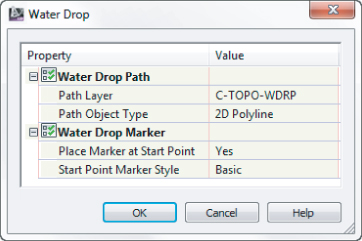
5. Verify that the Place Marker At Start Point option is set to Yes, as shown in
Figure 15.1, and click OK.
Note that you can choose a 3D or 2D polyline as the path type. You will keep this as 2D Polyline.
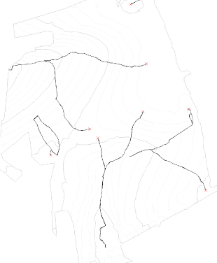
6. Get a feel for the site drainage by clicking on various areas throughout the site.
There is no wrong place to click, as long as you are inside the surface boundary. An X represents the place your cursor clicked. The place you click is a location on the surface where water hits the surface. You will see lines forming in the direction water flows from the area. If you see an X but no path, it could mean you are in a flat area or inside a small depression. After you click in several locations, your drawing will resemble
Figure 15.2.
7. Click around as many places as you would like to examine.
8. Press Esc to complete the Water Drop command.
9. Press Esc a second time to clear the surface selection.
The water drop paths that are created are polylines without any special intelligence. The following optional steps demonstrate how to remove them if your surface model changes or you need to clear them from the screen.
10. Select one of the X symbols and its corresponding water drop path. Be sure your surface is not selected.
11. Right-click and choose Select Similar.
All of the flow paths and corresponding Xs will be highlighted.
12. Remove them by pressing Delete on your keyboard.
Catchments
The first step in any runoff computation is finding the area of the watersheds (also known as drainage basins or catchments) that contribute to the flow.
Catchments work with your surface models to determine the area draining to a point you specify. They are also used to find the drainage path within the catchment to compute time of concentration (Tc).
Catchment Groups
You must create a catchment group before creating catchments. Catchment groups are a way to separate pre- and post-development watershed areas. Similar to sites, a catchment in one catchment group will not interfere with objects in another catchment group. Catchment groups do not interact with each other, allowing catchments from differing groups to overlay each other.
Catchment Creation
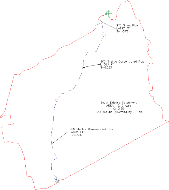
In Figure 15.3 you see a catchment with all its related features. You will need a grasp of the terminology used in the software before proceeding. It is useful to think about a hypothetical raindrop hitting the catchment to grasp what the various components represent.
Catchment Boundary
The outline represents the catchment boundary, often called the basin divide or watershed boundary. This represents the outermost points of the catchment object. Any raindrops that hit inside this boundary will flow to the same point.
Discharge Point
Toward the bottom of the boundary in Figure 15.3 is the discharge point. This is the main point of analysis used for the catchment. All raindrops that hit the basin ultimately end up at this location.
Hydraulically Most Distant Point
Near the top of the catchment boundary in Figure 15.3 is a marker indicating the hydraulically most distant point. A raindrop that lands at this point will take the longest to arrive at the discharge point.
Catchment Flow Path
In Figure 15.3, the catchment flow path is shown as a dashed line running through the catchment. This linear path represents the course the raindrop takes on its journey, from the hydraulically most distant point to the discharge point. The catchment flow path is used to determine the slope and length for computing the Tc for hydrology calculations.
Flow Path Segments
By default, a flow path is created with an average slope through its overall length. Using flow-path segments, you can break up the flow path into smaller pieces with the average slope computed per segment. Each segment can have different computation methods associated with them for Tc computations. The computation methods are as follows:
- SCS Shallow Concentrated Flow
- SCS Sheet Flow
- SCS Channel Flow
Time of Concentration
Time of concentration is the time it takes for a drop of rain to travel from the hydraulically most distant point to the discharge point. The default method for determining this value is TR-55. Civil 3D uses the flow type, slope, and user-specified Manning's roughness to determine the time. Alternately, you can input a user-defined time of concentration.
SCS, What? TR, Who?
TR-55 is short for a technical document put out in 1986 by a branch of the US Department of Agriculture. The agency prior to 1996 was called SCS (Soil Conservation Service), but is now known as NRCS (National Resources Conservation Service). Technical Release 55 “Urban Hydrology for Small Watersheds” is the seminal work behind hydrology computations in the United States.
This document, which has been added to the chapter dataset (which you can download from this book's web page) for your reference, describes the procedures needed for determining the curve number (a.k.a. runoff coefficient), when to apply the different flow types, and how to compute Tc for each flow type.
Civil 3D incorporates the Tc computation directly in the catchment object. However, TR-55 does have some limitations that you need to keep an eye out for in Civil 3D:
- Minimum time of concentration = 0.1 hour (6 minutes).
- If you're using sheet flow, it should be your first flow segment and should not exceed 300′ (91 m). Some newer literature says sheet flow should not exceed 200’ (60 m). Check with your local regulating authority for specific requirements. Typically, sheet flow morphs into shallow concentrated flow before 200’ (60 m).
- Each Civil 3D catchment supports one entry for curve number. However, the curve number is not used for determining the time of concentration. If you have nonhomogeneous land and/or soil types, leave the default, but be sure to compute the composite curve number in the SSA portion of the software.
- If you need to use a method other than TR-55 for Tc, you can specify User-Defined and leave the entry blank until you export to the SSA portion of the product.
Finally, keep in mind that Civil 3D catchments are not dynamic to the surface model. If the surface model changes, you will need to re-create your catchment.
Catchment Options
You can choose to create a catchment from a surface model or by converting a closed polyline. You will get the best results when defining your catchment by converting a polyline to a catchment area. Manually delineate your watershed areas using the Water Drop command you used in the previous section as a guide.
Create Catchment From Object
In most cases, this will be the method you should use for watershed creation. Use Create Catchment From Object if you have watershed data created ahead of time (i.e., from an imported GIS file or existing DWG). You will also need to use the Create Catchment From Object option for watersheds that are adjacent to your project's limits of disturbance. Even if you choose to use an existing polyline as the catchment boundary, you can still use the surface model to determine the flow path location and slope.
Create Catchment From Surface
Use the Create Catchment From Surface option if you have a well-formed surface model with adequate data for Civil 3D to compute the watershed area. Surface models with many flat areas, sparse data, or multiple hide boundaries will not work well for this tool. If you do not have good luck with this tool, don't be surprised. Make sure the surface model used for catchment creation is complete before defining a catchment object. The catchment is not dynamically linked to the surface model; therefore, it will not update if changes are made to the surface model.
If you are using the Hydrology tool on an existing ground surface (predevelopment), make sure all surveyed shots and breaklines are added before proceeding. If you are using the tools on a proposed site (postdevelopment), make sure corridor surface models, grading surface models, and any proposed elevation data are pasted together in the surface model used for analysis.
In the following exercise, you will use multiple tools to delineate several watershed areas for a predeveloped site. You will also use the site characteristics to specify Manning's roughness for SCS Sheet flow and SCS Channel flow. The site is covered in a dense grass.
1. Open the Catchment.dwg (or Catchment _METRIC.dwg) file, which you can download from this book's web page.

For this exercise you will find it helpful to turn on the Insert Osnap.
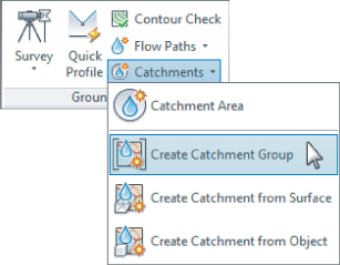
2. On the Analyze tab ⇒ Ground Data panel, choose Catchments ⇒ Create Catchment Group, as shown in
Figure 15.4.
3. Name the group Pre-developed. Click OK.
4. On the Analyze tab ⇒ Ground Data panel, choose Catchments ⇒ Create Catchment From Surface.
5. When you see the prompt Specify the Discharge Point:, select the insertion point of the storm structure labeled Existing Inlet (S).
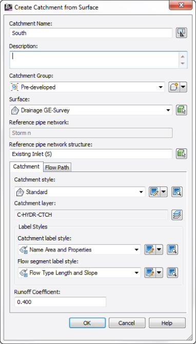
6. When the Create Catchment From Surface dialog appears:
a. Name the catchment South.
b. Set the surface to Drainage GE-Survey.
c. Click the Select Structure icon to set the Reference Pipe network structure to Existing Inlet (S). (Alternately, you can right-click to pick structures from a list.)
d. Set Catchment Label Style to Name Area And Properties.
e. Set Runoff Coefficient to 0.4. (This is the unitless runoff coefficient used in the Rational method.)
After a moment, a red line representing the catchment boundary will form.
7. Press Esc on your keyboard to dismiss the command.
8. On the Analyze tab ⇒ Ground Data panel, choose Catchments ⇒ Create Catchment From Object.
9. Select the closed polyline north of the first catchment.
10. At the prompt Select a polyline on the uphill end to use as a flow path (or Press Esc to skip):, click the eastern end of the blue, dashed polyline that runs across the catchment.
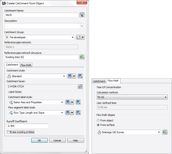
11. In the Create Catchment From Object dialog that appears:
a. Name the catchment North.
b. Click the Select Structure icon to set the Reference Pipe network structure to Existing Inlet (N).
c. Set Catchment Label Style to Name Area And Properties.
d. Set Runoff Coefficient to 0.4. (This is the same for both metric and Imperial units.)
e. Uncheck Erase Existing Entities. Your dialog will now look like the image on the left in
Figure 15.6.
f. Switch to the Flow Path tab.
g. Set Flow Path Slopes to From Surface.
h. Set Surface to Drainage GE-Survey.
Your Flow Path tab will now look like the image on the right in
Figure 15.6.
i. Click OK, and press Esc on your keyboard to exit the command.
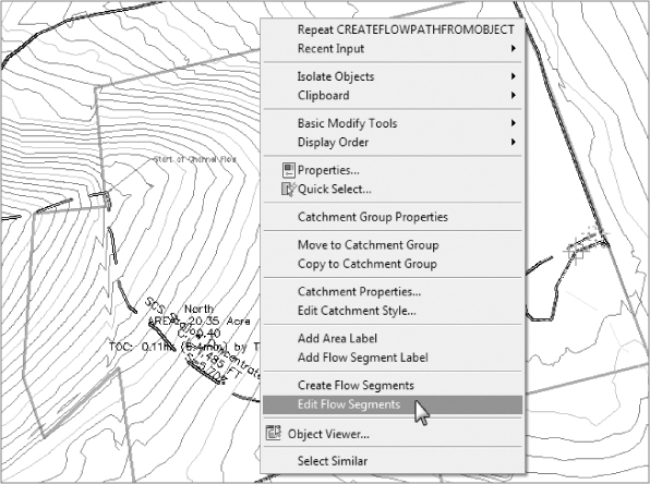
12. Select the North catchment by clicking anywhere on the red boundary, or on the dashed flow path line.
13. Right-click and select Edit Flow Segments, as shown in
Figure 15.8.
Panorama will appear showing the continuous path as SCS Shallow Concentrated Flow.
14. Change Surface Type to Short Grass Pasture.
15. Click the plus sign in the upper-left corner to create a flow segment.
16. Create the new flow segment by clicking at the location on the flow line labeled “Start of Shallow Concentrated Flow.”
The new segment is placed in the Panorama listing from uphill to downhill. Segment 1 is the segment you just created and Segment 2 represents everything else downhill. This new segment represents sheet flow.
17. Change the flow type for Segment 1 to SCS Sheet Flow. Note the input fields change to accommodate this type of flow.
a. Set the 2Yr-24Hr Rainfall value to 2.9″ (74 mm).
b. Set the Manning's Roughness value to 0.24 (Manning's roughness is a unitless value so this is the same for both metric and Imperial drawings).
The Manning's roughness for this area is based on coefficients for long grass found in the TR-55 document.
18. Click the plus sign and add the next segment at the abrupt bend in the flow path near the site boundary.
This is where our flow enters a swale.
19. For Segment 3, change Flow Type to SCS Channel Flow.
a. Set the Manning's Roughness value to 0.05.
b. Set the Cross-Sectional Area value to 27 ft2 (2.5 m2).
c. Set the Wetted Perimeter value to 28.2′ (8.6 m).
Manning's roughness was determined based on an earthen swale from TR-55. The cross-sectional area and wetted perimeter are site-specific measurements of the swale.
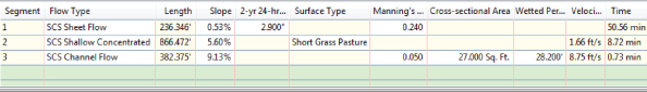
Your Panorama should now look like
Figure 15.9. You have used Civil 3D to compute the Tc for the north catchment.
20. Dismiss the Panorama by clicking the green check box in the upper-right corner. Save the drawing for use in the next exercise.
Exporting Pond Designs
One of the capabilities of SSA is to evaluate the performance of a detention pond during a storm event. Information about the pond's surface area at various depths must be collected. Civil 3D can easily compute stage-storage information from surface contours.
In Chapter 16, “Grading” you will learn all about creating proposed pond surfaces. In the following exercise, you will prepare a pond surface for export and generate the file needed to pass the information to SSA:
1. Open the file Proposed Pond.dwg or Proposed Pond_METRIC.dwg.
2. In the Prospector tab of Toolspace, expand Surfaces. Right-click Pond Surface and select Zoom To.
3. Click on one of the contours to bring up the Surface contextual tab.
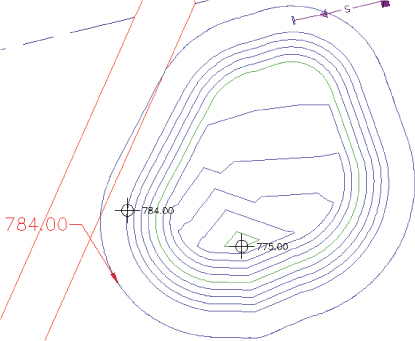
4. From the Surface Tools panel, click Extract Objects:
a. Uncheck Major Contour.
b. Change the Minor Contour Value drop-down to Select From Drawing, as shown in
Figure 15.10.
c. Click the Select From Drawing icon.
d. Pick the 784.0′ (239.0 m) elevation contour labeled with a red leader at the edge of the basin and press

.
5. Click OK.
A polyline is now generated from this contour.
6. Press Esc to clear the surface selection.
7. Expand Prospector ⇒ Surfaces ⇒ Pond-Eval Surface ⇒ Definition, and right-click Boundaries. Select Add.
8. Name the boundary Pond Top, clear the Non-destructive Breakline check box, and click OK.
9. Click the newly extracted polyline.
The surface is now narrowed down to the portion that is capable of holding water. The contours outside of this area have been omitted from the boundary, as shown in
Figure 15.11.
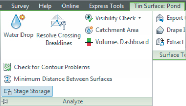
10. Again, select the surface to bring up the contextual tab.
11. From the Analyze panel flyout, select Stage Storage, as shown in
Figure 15.12.
12. In the Report Title field, type Pond-Eval. Leave all other options as default.
13. Click Define Basin.
14. In the Basin Name field, type Pond1.
15. Verify that Define Basin From Surface Contours is toggled on, as shown in
Figure 15.13.
16. Click Define.
17. Select the surface by clicking any of the contours.
18. Click Save Table, and save the file to your Mastering Civil 3D folder as Pond-Eval.
The file type will be AECCSST, which is a special format used by SSA.
19. Close the Stage Storage dialog by clicking Cancel.
In the SSA-focused portion of this chapter, you will use the stage-storage table to see if your pond floods during a storm event.
Exporting Pipes to SSA
When your catchments and your pipe networks are ready to be analyzed, switch to the Analyze tab and select Edit In Storm And Sanitary Analysis. You must have at least one pipe to export.
When you export, the pipe network information, inlets, pipes, and elevations convert over to SSA. Catchment data is shown with area, Tc, and runoff coefficient as data only. The graphic area that you define on the Civil 3D end is not needed.
When you first export a project over, SSA will ask if you would like to create a new project or open an existing project. If you are adding pipes to an existing network that has been analyzed in SSA, click the Open Existing Project radio button and browse to the location of your stored SPF file.
When you create a new project, SSA does a few grunt-work things for you. First, it converts all your junctions and pipes to the SSA format (via Hydraflow's STM file, oddly enough) and asks if you would like to save the log file. Generally, saving the log file is not necessary unless you are having difficulty importing certain objects. In most cases, you can click No to continue.
Once you are in the SSA interface, you can access your active project by clicking the Plan View tab at the top of the window. You will see your DWG file as an underlay to the project you are working on.
How Does SSA Decide What's an Inlet and What's a Manhole?
Buried deep in the bowels of your command settings are the Part Matchup settings.
1. Start a new drawing based on the template of your choice. On the Settings tab, choose Pipe Networks ⇒ Commands and double-click the EditInSSA option.
2. Once you are there, expand the Storm Sewers Migration Defaults area.
3. Click the Part Matching Defaults field.
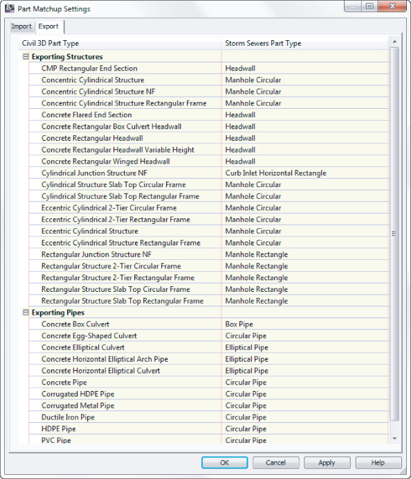
4. Click the ellipsis to enter the Part Matchup Settings dialog.
The Import tab handles how parts from SSA or Hydraflow behave on the way into Civil 3D. The Export tab handles how SSA or Hydraflow handles parts from Civil 3D. As you can tell from poking around here, there isn't always a perfect match for every part you use.
There are a few quirks and limitations with the intended SSA workflow:
- Pipe networks that contain parts from multiple-part families (for example, a pipe network may contain a part from the HDPE family and another part from the Concrete family) will reimport back into Civil 3D with only one part family.
- To prevent SSA and Civil 3D from changing your pipe sizes, make a single part family for all circular pipes. Be sure that the “master” part family contains all possible sizes. Once it is reimported back to Civil 3D, use Swap Part to change back to the original part family type.
- For advanced users, there is a super-secret XML file located in C:Program Files(x86)AutodeskSSA 2013SamplesPart Matching. For more information about using and editing this file, see the Part Matching help file.
- Culverts are treated the same as a single pipe in SSA. Once you export a culvert into SSA, you'll need to set entrance and exit conditions.
A little part tune-up will be needed after the round-trip; however, the time savings in using the export commands are still very much worth it.
Storm and Sanitary Analysis
SSA can perform a number of water- and wastewater-related tasks. In the remainder of this chapter, you will be going through several examples of what SSA can do, but you are just seeing the tip of the proverbial iceberg.
In this section, you will focus on the workflow between Civil 3D and SSA. First, you will learn how to create subbasins (catchments) directly in SSA. You'll also see examples of the Rational method and TR-55, and learn about SSA reports.
Guided Tour of SSA
SSA is a separate program that is optionally installed with Civil 3D. To get into SSA you can launch it from the desktop icon, from the Start menu, or from the Analyze tab in Civil 3D.
SSA is not at all like AutoCAD®. It is a true modeling software program that shows a schematic of your design in a plan view. On the left side of the screen you will see the data tree (Figure 15.15). Like Prospector in Civil 3D, the SSA data tree gives you access to tools and information about objects.
The easiest way to add new structures, pipes, or catchments to the project is to do so from the Elements toolbar along the top of the screen. Here, you will find everything you need to build a project from scratch if you did not start out in Civil 3D.
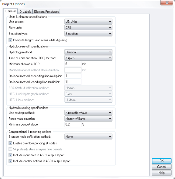
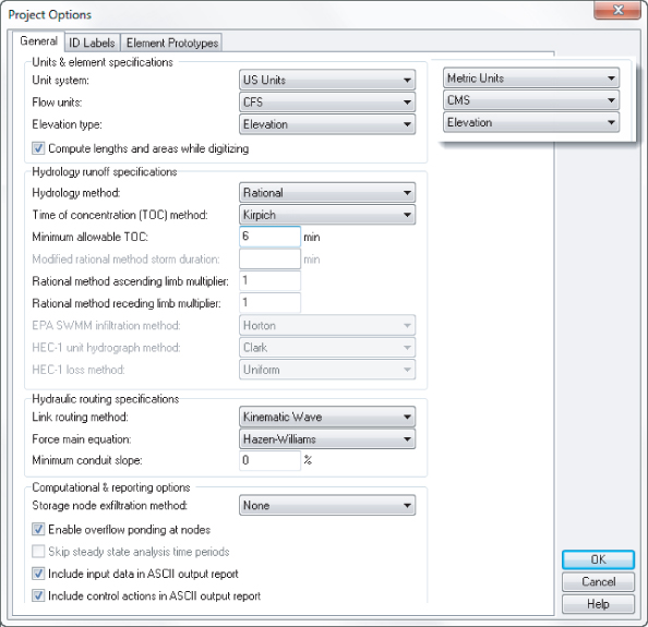
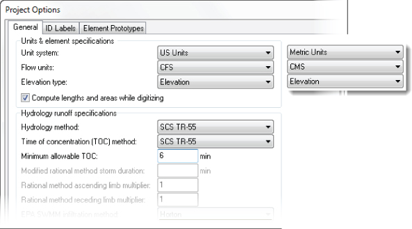
The next stop on our tour is the Project Options dialog (Figure 15.16). Access this dialog by double-clicking on the Project Options listing in the data tree. The General tab of the Project Options dialog is where you set your units, hydrology method, routing method, and force main equation. Depending on the scope of your project, you may not need to worry about every setting.
A Few Hints for Working in SSA
Since this is not traditional CAD, the program behaves differently than you might expect. This list contains a few hints to help you along the way:
- Make sure you download and install the Civil 3D 32-bit object enabler. SSA needs the object enabler to see Civil 3D objects such as pipes, structures, and nodes. Since SSA is a 32-bit application under the hood, you should download the 32-bit version of the object enabler even if your computer is on a 64-bit operating system.
- Unlike AutoCAD, SSA keeps you in a command until you press Esc or click the Select Element tool from the toolbar.
- Be mindful of the tabs along the top of the screen. To dismiss them, use the red X that appears on the tab itself. It is a common mistake to dismiss the program accidentally by clicking the incorrect red X.
- Don't forget to save! Unlike CAD, there is no auto-save.
- Work upstream to downstream.
- There is no Undo command in SSA. Luckily, adding and removing elements is a simple process. If something gets goofed up beyond repair, you could always close without saving.
It may take a while to get used to, but SSA is a powerhouse analysis tool.
In one of the upcoming examples, you will use the Rational method with TR-55 Tc calculations. Since you are calculating runoff only, you do not need to set the other project options. Once you have finished entering the options shown in Figure 15.16, click OK.
Whenever you are designing in SSA, always work upstream to downstream. If your system includes a pump, you should work from highest elevation to lower elevations.
An SSA project consists of three main object types: subbasins, nodes, and links:

Subbasins
Subbasins are important for runoff computations, but are not mandatory if you are inputting flows manually. Subbasins can be defined directly in SSA or brought over as data from Civil 3D. SSA can also turn an SHP file directly into a subbasin.
Nodes
Nodes are where all calculations are done in SSA. If you want information along a pipe, for example, you will need to place a junction node at the location of interest.
Nodes are the workhorses of SSA, and can take several forms:

Junction Node
When SSA converts structures from Civil 3D, it assumes a junction node by default. These can be used as manholes, null structures, water, or pollutant infiltration or treatment points. Junctions are frequently used to consolidate links that would flow to the same outfall. Junctions can connect many links, but outfalls cannot.

Outfall Node
Outfall node is the end of your system. An outfall can be a culvert discharge location, where a proposed sewer ties into an existing one, or where sanitary sewer enters a treatment facility. An outfall can be attached to only one link.

Flow Diversion Node
If a node has two outgoing links, you will need to use a flow diversion. Flow diversions most commonly represent multiple outflow points on a detention basin, such as a weir or orifice. They can also represent flow diversion in a combined sewer system or anywhere an overflow check is in use.

Inlets
Inlets are used in storm systems and can collect flow from a subbasin. You can also manually enter flows.
Inlets are either on grade or in sag. For inlets on grade, a downstream link must be specified. The downstream link (i.e., curb and gutter between storm inlets) tells the software where water goes if the current inlet cannot handle the rainfall.
Inlets in sag are assumed to pond in a storm event and do not need downstream links associated with them.

Storage Nodes
Anywhere water is detained on your site, a storage node can model the scenario. Storage nodes can represent ponds, wet wells, underground storage, or a residential rain barrel.
Later in this chapter you will use a storage node to model headwater effects on a culvert.

Links
Any time water is moved from place to place, it does so via links. Links connect nodes to each other. Links represent pipes, channels, curbs and gutters, or culverts.

Pumps
Pumps can be used to push water uphill. They can be built to start functioning when the water at a storage node reaches a certain depth using operational controls. When using a pump link, you can work in design mode when specific pump data is not available. As pump data becomes available, you should enter pump curve data to tell SSA how much “oomph” the pump has.

Weirs and Orifices
Weirs and orifices both allow water to flow out of a storage structure at a controlled rate.

Outlet
An outlet is a node type that can be used where weirs or orifices are too simple to model discharge from a storage node. An outlet can have a rating curve or discharge function associated with it.
Hydraflow, We Haven't Forgotten You
When it comes to flexibility in storm design and routing, SSA beats the pants off Hydraflow any day. In general, there is a lot of overlap between the two products. For basic storm sewer calculations, either product will work great. When your designs get more complex and require hydrograph and storage routing with infiltration and exfiltration, SSA has a much better solution.
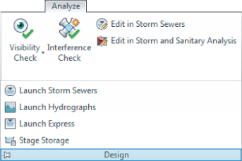
You can still access all the Hydraflow functions from the Analyze tab ⇒ Design panel flyout.
Hydraflow is still part of the picture when it comes to exporting and importing data to and from Civil 3D. Hydraflow's file format does a much better job than LandXML at keeping the data integrity of your pipes and structures.
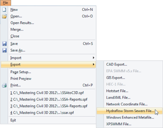
When exporting from SSA, choose File ⇒ Export ⇒ Hydraflow Storm Sewers File for the best path back to Civil 3D.
Hydrology Methods
SSA is capable of computing rainfall runoff using any of the following methods:
Rational Method
The Rational method is used to approximate the peak discharge (or flow, Q) from an impervious area (A) using the tried and true Q=ciA. This is the most common method used for sizing sewer pipes.
Imagine yourself outside in a rainstorm, staring at a single point on your driveway (assuming your driveway is impervious and on a nice, even slope). At first, the water on your driveway is coming right from the sky. After a while, water flows in from rain falling elsewhere in your neighborhood. Now imagine that the storm stops as soon as raindrops from the farthest point in your neighborhood reach the point on your driveway.
The Rational method is based on the assumption that it takes the same amount of time for those farthest raindrops to get to you as they do to run off your driveway completely.
The first step to using the Rational method is to delineate the drainage basin, as described earlier in this chapter, and assign composite runoff coefficients. SSA needs an intensity-duration-frequency (IDF) curve for the study area to compute the rainfall.
Modified Rational and DeKalb Rational
These hydrology methods are similar to the Rational method, except that they are intended to approximate the storage volume needed on small, simple detention basins. Instead of the storm duration equaling two times the time of concentration, the storm duration is longer. The longer storm duration results in a larger volume than the Rational method but results in a lower peak discharge.
The same information is needed for the Modified and DeKalb Rational methods as for the Rational method, and you must have a value in the Project Options dialog for Modified Rational Storm Duration.
Both the Rational method and the Modified Rational method are intended for small watersheds, usually less than 20 acres (8.1 hectares).
SCS TR-55 Method and TR-20 Method
More gifts from the USDA, the SCS TR-55 runoff method is a more complex method that is appropriate for study areas up to 2,000 acres (809 hectares).
For the SCS TR-55 and TR-20 methods, SSA contains tools for looking up computation variables. You will find a curve number (CN) lookup table inside the subbasin. SSA will even help you determine the composite curve number. The TR-55 hydrology method is also where you will use SSA rain gauges.
HEC-1
The US Army Corps of Engineers' Hydraulic Engineering Center has a computer program called HEC-1 for hydrology calculations. The HEC-1 method in SSA duplicates the results from the Army Corps' program. Their method is used in situations where there is an existing body of water, such as a stream. For an explanation of this method directly from the source, go to http://www.hec.usace.army.mil/publications/TrainingDocuments/TD-15.pdf.
EPA-SWMM
The US Environmental Protection Agency (EPA) Storm Water Management Model (SWMM) method is used for developed watershed areas and can take into account many more factors than the other analysis methods. SWMM allows for localized ponding effects, which can be entered into the subbasin physical properties area. This method also allows for the effects of existing soil moisture, evaporation, and snowmelt in the system. When using EPA-SWMM, be sure to set all the methods you intend to use for infiltration and exfiltration in the Project Options dialog.
In the following example, you will work through a simplified example to get the feel for the SSA interface:
1. Launch SSA from the stand-alone icon in your computer's Start menu or from the desktop. Open the file SSA Intro.spf or SSA Intro_METRIC.spf, which you can download from this book's web page.
2. In the SSA interface, choose File ⇒ Import ⇒ Layer Manager (DWG/DXF/TIF/More), as shown in
Figure 15.17.
This will bring up the Layer Manager, where you can import a DWG as a background.
3. Click the ellipsis next to the Image/CAD File field.
4. Browse to the file SSA Intro.dwg (or SSA Intro_METRIC.dwg) file, which you can download from this book's web page.
5. Place a check mark next to Watermark Image and click OK.

6. Click the green Add Subbasin button from the elements toolbar along the top of the window.
7. Using this tool, click around the boundary lines that represent the example watersheds.
8. When you are close to completing a shape, right-click and select Done to close the shape.
There are no snap or curve drawing tools in SSA. Digitize as closely as possible using multiple small segments. If you make a mistake, you can right-click and select Delete Last Segment.
When you have completed both shapes, your graphic will resemble
Figure 15.18.

9. Switch to the Inlet tool by clicking the Inlet button at the top of the SSA window.
10. Working upstream to downstream, (left to right in this case), place two inlets on the south side of the site.
An X has been placed at each inlet location to help you locate the recommended positions.
11. When you have finished placing inlets, press Esc on your keyboard or click the arrow icon in SSA to get back to Selection mode.
If you accidentally place more inlets than you wanted, you can right-click the wayward inlet while in Selection mode and select Delete from the menu.
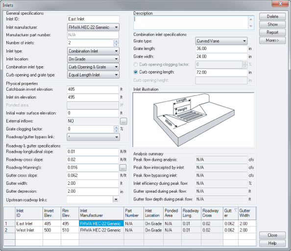
12. Double-click one of the inlets to enter the Inlets dialog:
a. Rename the first inlet you placed to West Inlet.
b. Set Number Of Inlets to 2.
c. Change Invert Elevation to 500′ (152.4 m).
d. Change Rim Elevation to 510′ (155.4 m).
e. Use the table at the bottom of the dialog to switch to the second inlet, and rename the second inlet to East Inlet.
f. Set Number Of Inlets to 2.
g. Change Invert Elevation to 485′ (147.8 m).
h. Change Rim Elevation to 495′ (150.9 m).
Leave all other settings at their defaults, as shown in
Figure 15.19, and close the Inlets dialog.

13. Click the Outfall icon. Click to place the outfall structure in the location marked with a circle at the southeastern corner of the site.
14. Press Esc to return to the selection tool.
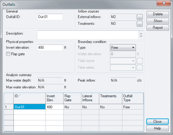
15. Double-click the new outfall to enter the Outfalls dialog:
a. Set the Invert Elevation value of the outfall to 480′ (146.3 m).
b. Set the Boundary Condition type to Free, as shown in
Figure 15.20.
c. Leave all other options at their defaults, and click Close.

16. Switch to the Conveyance Link tool.
17. Working from left to right across the project, click the upstream inlet. (Resist the temptation to click and drag.)
18. Connect the first inlet with a straight segment to the second inlet.
19. Connect the second inlet to the outfall.
20. Press Esc to return to the selection tool.
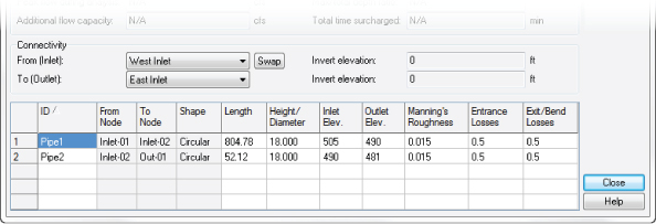
21. Double-click the first conveyance link you created.
You will see the Conveyance Links dialog. The easiest place to rename the pipes is in the small grid at the bottom of the box, as shown in
Figure 15.22. When your cursor is in the field to rename a pipe, a dark black square will appear on the pipe in the main graphic, helping to indicate which pipe you are editing. Your initial numbering may vary, so you will rename the pipes in the steps that follow.
22. Rename the first link to Pipe1. Rename the second conveyance link to Pipe2, and then click Close.
So far, you've told SSA what your drainage areas are and you've established a pipe network. Next, you need to tell SSA which subbasin drains to which inlet.
23. Switch to the selection tool by pressing Esc if it is not already active.
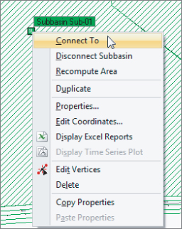
24. Right-click the icon that represents the western subbasin and select Connect To, as shown in
Figure 15.23. If you receive a dialog box message with the “Connect To” help message, clear the check box and click OK.
25. Connect the subbasin to the western inlet by clicking the inlet symbol in plan view.
A line will form to indicate the connection was successfully created.
26. Repeat the process for the eastern subbasin and inlet.
At the end of the process your SSA screen will resemble
Figure 15.24.
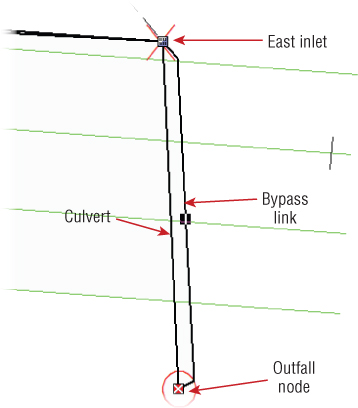
Before SSA can run any analysis on the project, you must make one last crucial connection. Both of these inlets are on grade, which means water will flow toward them, but in a big storm, some water may flow past into the next downstream inlet. The flow along the gutter of the road between inlets is called a bypass link.
27. Click the Add Conveyance Link button.
28. Connect the west to the east again, but this time follow the curve of the road.
This conveyance link represents the gutter flow of any water that doesn't make it into the west inlet and continues on to the eastern, downstream inlet.
29. Add a conveyance link between the east inlet and the outfall.
To visually differentiate the culvert from the bypass link, you can put a small kink in the line, as shown in
Figure 15.25. When you modify link properties, you will have the opportunity to compensate for the change in length this technique causes.
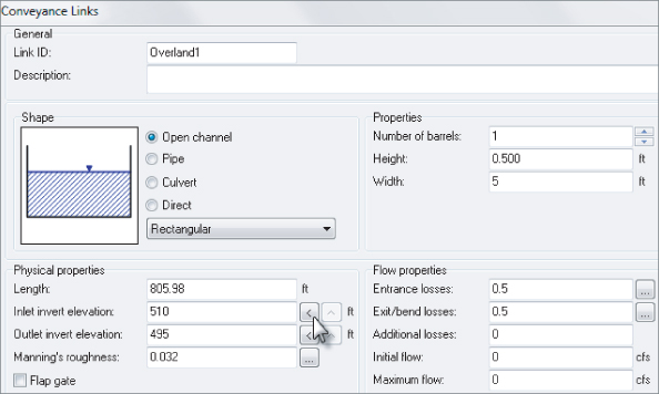
30. Rename the new links to Overland1 and Overland2, respectively.
Overland1 and Overland2 represent surface flow along the gutter and over the road. For this example, you will approximate the flow using a rectangular open channel.
31. Set the shapes of both Overland1 and Overland2 from Pipe to Open Channel, as shown in
Figure 15.26.
a. Set Height to 0.5′ (0.15 m).
b. Set Width to 5′ (1.5 m).
Now that these conveyance links are set to Open Channel, SSA recognizes that they must be surface-flowing channels. In the next step you will update the curb and gutter elevation to reflect the top of the inlets.
32. For both Overland1 and Overland2:
a. Click the arrow button next to Inlet Invert Elevation.
b. Click the arrow button next to Outlet Invert Elevation.
The elevations should update to reflect the rim elevations of the inlets. (You set these values back in step 12.)
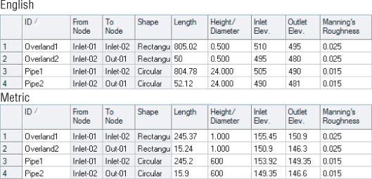
33. Using the tabular input at the bottom screen, enter the values for Diameter, Inlet Elevation, Outlet Elevation, and Manning's Roughness, as shown in
Figure 15.27. Leave all other options at their defaults, and click Close when you are done.
All the pieces are here; next you will verify the connections to the pipes, inlets, outfalls, and curb flows.
34. Double-click one of the inlets to return to the Inlets dialog.
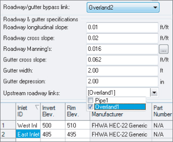
a. For West Inlet, set Roadway/Gutter Bypass Link to Overland.
b. For East Inlet, set Roadway/Gutter Bypass Link to Overland2, as shown in
Figure 15.28.
c. Click Close when complete.
Now that all the elevations are set, you must tell SSA how much rain you expect to see in your system.
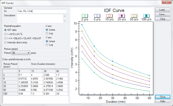
35. In the data tree on the left side of the SSA window, in the Hydrology branch, double-click IDF Curves, as shown in
Figure 15.29.
36. Click Load, and browse to the file York Co PA.idfdb (or York Co PA_METRIC.idfdb) and choose Open.
This is the rainfall data for our example file, which you can download from the book's web page.
37. After loading the file, set the ID to
York, PA, USA, as shown in
Figure 15.30. Click Close.
38. In the data tree on the far left, double-click Project Options.
a. Set Hydrology Method to Rational.
b. Set Time Of Concentration (TOC) Method to Kirpich.
c. Set your minimum allowable TOC to 6 minutes.
d. When your Project Options dialog resembles
Figure 15.31, click OK.
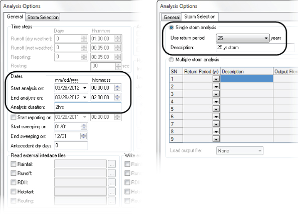
39. Double-click Analysis Options from the data tree.
a. On the General tab, set the End Analysis On value to 02:00:00.
Your dates will vary from what is shown in
Figure 15.32, but the important thing is that the duration of the analysis is long enough to accommodate the Rational method.
b. On the Storm Selection tab, set Return Period to 25 years for a single storm analysis.
c. Click OK when complete.
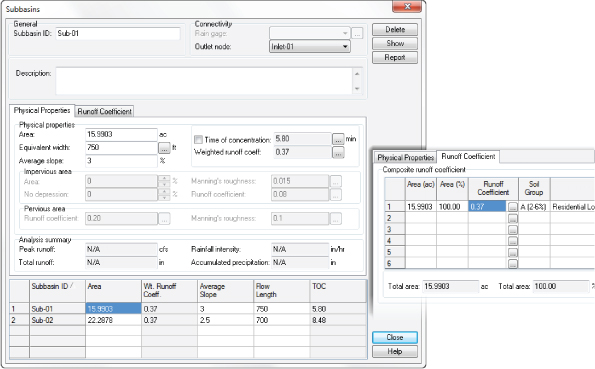
The last step before you are ready to run the design is setting the subbasin information for use with the Kirpich method of time of concentration. The Kirpich method calculates Tc based on the average slope and area characteristics of the site.
40. Double-click the green subbasin icon located in the centroid of the western subbasin.
a. For the western subbasin, set the flow length to 750′ (228.6 m), and set the average slope to 3%.
b. Switch to the Runoff Coefficient tab and set the runoff coefficient to 0.37.
c. Switch to the eastern subbasin by selecting its row at the bottom of the dialog.
d. Set the eastern subbasin flow length to 700′ (213.4 m), and set its average slope to 2.5%.
e. Switch to the Runoff Coefficient tab and set the runoff coefficient to 0.37.

41. Click Perform Analysis.
After a moment, the analysis will complete.
42. Click OK.
In the SSA graphic, you will see a heavy, blue line indicating that conveyance link Overland1 is flooded. Later on in the chapter you will look at reporting capabilities to see the details of this predicament.
43. Save the file as SSA1.spf and close. Close SSA in preparation for the next exercise.
From Civil 3D, with Love
Earlier in this chapter, you saw some of the preparations that must take place before you click the Edit In Storm And Sanitary Analysis button. Once inside SSA, a few more pieces of information need to be added before SSA can do its analysis.
In the following example, you will see what becomes of catchment objects and pipes once they are imported into SSA:
1. From Civil 3D, open the file C3DtoSSA.dwg (or C3dtoSSA_METRIC.dwg). You can download this file from the book's web page.

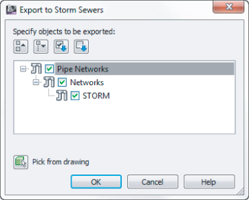
2. Select the Analyze tab ⇒ Design panel and click Edit In Storm And Sanitary Analysis.
3. Verify that there is a check mark next to the STORM pipe network.
4. Click OK in the Export To Storm Sewers dialog, as shown in
Figure 15.34.
5. SSA launches. Click OK to create a new project.
After a moment, SSA will let you know that you have successfully imported the Hydraflow Storm Sewers file.
6. Click No—you do not need to save the log file.
7. At the top of the SSA window, click Plan View.
8. Examine the inlets and catch basins that have been imported.
Notice that an offsite outfall has been added to each inlet. This is because you don't model the overland links in Civil 3D. When inlets are first imported into SSA, the program assumes they are on grade. Water that bypasses on grade inlets needs to go somewhere, so SSA automatically throws in an outfall to take care of the excess water. In the next steps you will remove the outfalls and create the overland links.
9. Right-click on the outfall that has been added to Inlet Structure - (1).
11. Click Yes to confirm the deletion.
12. Right-click and delete the outfall to the far right. Click Yes to confirm the deletion.

13. Add overland conveyance links similar to the previous exercise:
a. Add a link between Inlet Structure - (1) and Inlet Structure - (2).
b. Add a link between Inlet Structure - (2) and the outfall.
14. Double-click one of the conveyance links to edit the links in tabular form.
15. Set the diameters of Pipe - (1) and Pipe - (2) to
24″ (
600 mm), as shown in
Figure 15.36.
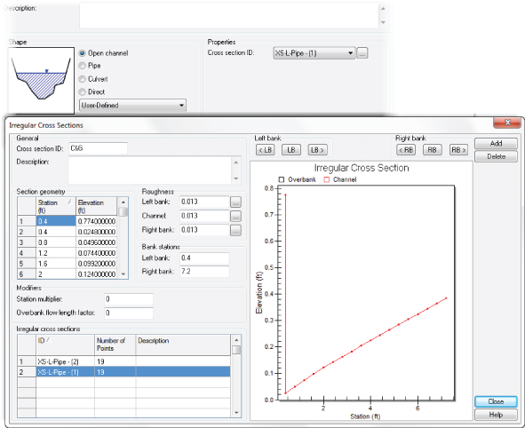
16. Select the row for either one of the overland links.
a. Change the channel type to Open Channel.
b. Set the shape type to User-Defined, as shown in
Figure 15.37.
c. Set the Cross Section ID to XS-L-Pipe - (1).
d. Click the ellipsis next to XS-L-Pipe - (1) to open the Irregular Cross Sections dialog.
The shape you see in
Figure 15.37 is an exaggerated view of a curb and gutter. In the previous example, you approximated the curb and gutter channel using a rectangular open channel. In this exercise, you will use one of the cross sections created for you by the export process.
17. Rename the Cross Section ID to C&G. Close the Irregular Cross Section dialog.
18. Make sure both Link-01 and Link-02 are using the C&G cross section for open channel flow by setting the Cross Section ID for each.
19. Click Close when your conveyance links are complete.
20. Double-click Project Options in the data tree.
a. Set the Hydrology method to SCS TR-55.
b. Set the Time Of Concentration method to SCS TR-55.
c. Set Minimum Allowable TOC to 6 minutes.
At the end of this step, your Project Options dialog should look like
Figure 15.38.
21. Click OK.
22. Back in plan view, double-click the west subbasin icon.
23. Switch to the SCS TR-55 TOC tab. You will enter the following information to compute TOC for the western subbasin:
a. On the Sheet Flow subtab, set the Manning's roughness value for Subarea A to 0.17.
This value is based off the TR-55 listing for different land conditions. The listing of values can be found by selecting the ellipsis next to the entry field.
b. Set Flow Length to 150′ (45.7 m).
c. Set Slope to 5%.
This is another site-specific value and represents the average overall slope of the subbasin.
d. Click the ellipsis next to the 2Yr-24Hr Rainfall, and in the resulting dialog, choose Pennsylvania from the State drop-down, and York from the County drop-down, as shown in
Figure 15.39. (Metric users, enter a value of
79 mm for rainfall value, because this specification is only reported in inches.)
e. Click OK.
Selecting the rainfall location at this point is helping you determine the Tc. Your actual design storm duration may vary. Later in this chapter you'll learn more about rainfall.
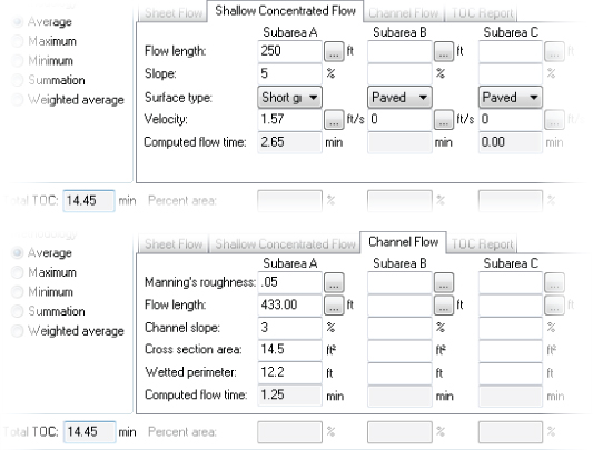
24. Switch to the Shallow Concentrated Flow subtab for Subarea A.
a. Set Flow Length to 250′ (76.2 m).
b. Set Slope to 5%.
c. Set the surface type to Short Grass Pasture.
The velocity for sheet flow will calculate based off the nomograph, which you can examine by clicking the ellipsis button next to Velocity. Your results should resemble the top of
Figure 15.40.
25. Switch to the Channel Flow subtab and set the Manning's roughness value for Subarea A to 0.05.
a. Set the flow length to 433′ (131.9 m).
b. Set the channel slope to 3%.
c. Set Cross Section Area to 14.5 ft2 (1.35 m2).
d. Set Wetted Perimeter to 12.2′ (3.7 m).
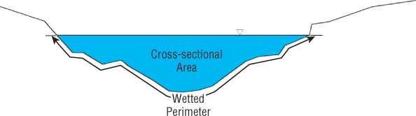
Wetted Perimeter and Cross Section Area are site-specific values and are needed to calculate the hydraulic radius used in the Manning's roughness equation.
Figure 15.41 shows a schematic of what these values mean in channel flow.
After entering the values for channel flow, your dialog will now resemble the bottom of
Figure 15.40.
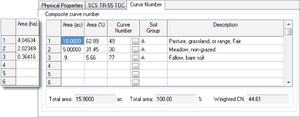
26. Still working with Sub-Structure - (1), switch to the Curve Number tab.
27. Set the curve number values for the subbasin as shown in
Figure 15.42.
28. Switch to the eastern subbasin by highlighting Sub-structure - (2) in the tabular listing near the bottom of the dialog. The Tc parameters for this subbasin are:
- Sheet Flow: Manning's Roughness of 0.17, Flow Length of 200′ (61.0 m), and Slope of 4.5%
- Shallow Concentrated Flow: Flow Length of 412′ (125.6 m), Slope of 4%, and Surface Type set to Short Grass Pasture
- Channel Flow: Manning's Roughness of 0.05, Flow Length of 305′ (93.0 m), Channel Slope of 2%, Cross Section Area of 12.2 ft2 (1.13 m2), Wetted Perimeter of 8.4′ (2.5 m).
29. Still working with Sub-Structure - (2), switch to the Curve Number tab and set the curve number to 45 for the entire area.
30. Click Close. Save the file as C3DtoSSA.spf for use in the next exercise.
Make It Rain
There are several methods for telling SSA the rainfall information for the model. A typical rainfall event in Herten, the Netherlands, is going to be vastly different from Phoenix, Arizona.
In the previous exercise, you set up many of the physical characteristics of the hydrologic system. You did not, however, tell SSA what type of rain to expect on the site.
Different hydrology methods require different assumptions about rainfall. In the Rational method, you used an intensity-based rainfall model (IDF Curve) because you were primarily interested in peak runoff. Because this is a TR-55 example, you will need to use rainfall information appropriate for this method.
1. Continue working in the file from the previous exercise or open SSA-Rain.spf (or SSA-Rain_METRIC.spf) in the Storm And Sanitary Analysis program.
You can download this file from the book's web page.

2. From the top of the SSA screen, select Add Rain Gauge.
3. Click anywhere in plan view to place the rain gauge in the project.
4. Press Esc on your keyboard to return to Selection mode.
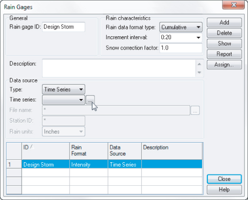
5. Double-click the New Rain gauge, and rename the Rain Gauge to Design Storm.
a. Set Rain Data Format Type to Intensity.
b. Set Incremental Interval to 0:20.
At this step your Rain Gauge dialog will look like
Figure 15.43.
6. Click the ellipsis next to Time Series.
7. In the Time Series dialog, click Add.
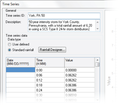
8. Rename the Time Series to York, PA 50.
9. Set the data type to Standard Rainfall and click the Rainfall Designer button.
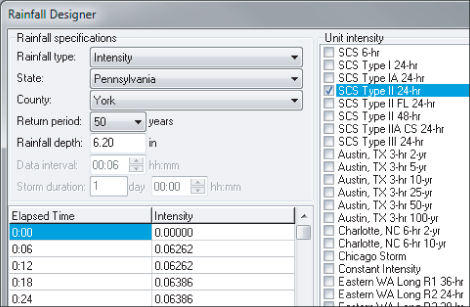
a. Set Rainfall Type to Intensity.
b. Set State to Pennsylvania and County to York.
c. Set Return Period to 50 years.
10. Make sure that the Unit Intensity check box next to SCS Type II 24-hour is selected, as shown in
Figure 15.44. (Metric users, override the Rainfall Depth by entering
157 mm.) Click OK.
11. Once your Time Series dialog resembles
Figure 15.45, click Close.
12. In the Rain Gauge dialog, click Assign.
a. Click Yes when asked if you'd like to assign the rain gauge to all subbasins.
b. Close the Rain Gauge dialog.
13. Double-click Inlet Structure - (1). Expand the Inlet ID column to get a better view of the table.
14. Set Roadway Gutter Bypass Link to Link-01.
15. Switch to Structure - (2) by selecting it from the table at the bottom of the Inlets dialog.
16. Set Roadway Gutter Bypass Link to Link-02, and click Close.

17. Double-click Analysis Options on the data tree.
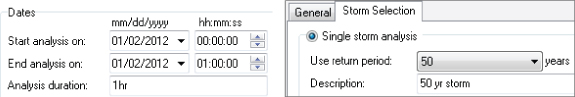
18. On the General tab, set the Analysis Duration to 1d by changing the date in the End Analysis On field to one day after the value in the Start Analysis On field On (the exact date will vary depending on when you open the file).
19. On the Storm Selection tab, set Single Storm to Use Assigned Rain Gauge, and click OK.

20. Click Perform Analysis.
21. After the analysis runs successfully, click OK. Save and close the project.
Culvert Design
In SSA, culverts can be modeled with great accuracy by treating them like a dam. If you think about it, that is exactly what is happening; the road acts like a dam between flow locations and the culvert is a hole connecting the two sides. During a storm event, water backs up and is stored until the culvert can release it or the road floods. If the water elevation on the high side goes over the road, this is similar to a weir releasing water over a dam.
In this exercise, you will work through the steps of designing a culvert. Several important steps have already been completed for you:
- The Project options have been set to use the Modified Rational hydrology method.
- Watershed areas have been delineated and associated with respective inlets.
- The local IDF curve has already been imported and saved with the drawing.
1. From SSA, open the file Culvert.spf (or Culvert_METRIC.spf), which you can download from this book's web page.
This file contains four subbasins that will drain through a culvert to the final outfall. The culvert portion of the project is incomplete.
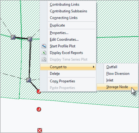
2. Right-click on the node Junction1, and select Convert To ⇒ Storage Node, as shown in
Figure 15.46.
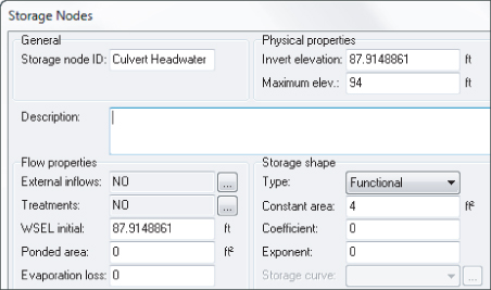
3. Once the storage node has been converted, double-click the node.
a. Rename the storage node to Culvert Headwater.
b. Verify that the Storage shape type is Functional.
This means that the area of the storage node can be described as a function of the depth.
c. Set the Constant Area to 4 ft2 (0.37 m2).
We are assuming that the last junction before the culvert has storage capability. A constant area is indicating that the junction is a vertical walled structure with a floor area of 4 ft2 (0.37 m2).
d. Set the Coefficient to 0.
e. Set the Exponent to 0.

5. Click the Add Conveyance Link tool.
6. Connect the storage node to the remaining junction.
7. Connect the remaining junction to the outfall.
8. Press Esc to exit the conveyance link tool.
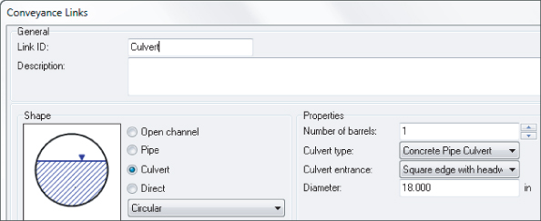
9. Double-click the link that connects the storage node to the junction.
a. Rename the Link ID to Culvert.
b. Set the Shape toggle to Culvert.
c. Leave the diameter to the default
18″ (
450 mm), as shown in
Figure 15.48.
10. Close the Conveyance Link dialog.
Next, you will add a weir to the storage structure. A weir is used to model what happens when water rises above the maximum storage elevation and runs over the street.

11. From the Elements toolbar, click Add Weir.
12. Draw the weir in the same manner as you drew the overland links in the previous exercise.
13. Add an extra segment to differentiate it visually from the main culvert link. Press Esc.
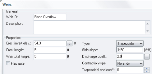
14. Double-click the new weir:
a. Rename the weir to Road Overflow.
b. Set the crest invert elevation to 94.3′ (28.7 m).
This elevation represents the roadway crown elevation at the culvert crossing.
c. Set the crest length to 5′ (1.5 m).
d. Set the weir total height to 5′ (1.5 m).
e. Set the type to Trapezoidal.
f. Set the side slope to 1:50.
g. Set the discharge coefficient to 2.9.
h. Set the contraction type to No Ends.
i. Set the trapezoidal end coefficient to 0.
Because this not a true weir or spillway, you are entering the above values to mimic the long, flat characteristics of a roadway.
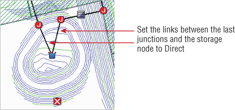
16. Double-click the southernmost link that connects the junction to the outfall.
The extra link to the outfall is needed because an outfall can only be connected to one link in SSA. You will use the Direct option to indicate that no head loss or time is contributed to the system in this link.
17. Change Shape to Direct. Leave all other options at their defaults, and click Close.
Now that all the physical characteristics of the model are in place, it is time to check the environmental aspects. You already have the IDF curve in place, but you still need to enter time of concentration and runoff coefficients to the subbasins.
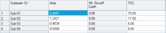
18. Double-click any of the green subbasin icons.
19. Set the Runoff Coefficient to 0.88 for all four subbasins to reflect a commercial (highly impermeable) site.
20. Set the time of concentration for each subbasin as shown in
Figure 15.50. Times will be the same for both metric and Imperial, but the area value will differ.
21. Close the Subbasin dialog when complete.
22. Double-click Analysis Options.
a. On the General tab, change the End Analysis time to
01:00:00, as shown in the left image in
Figure 15.51.
Note that you cannot change the Analysis duration field directly—you need to change the time.
b. On the Storm Selection tab, set the storm return period to 50 years, as shown in the right image in
Figure 15.51.
23. Click OK to close the Analysis Options dialog.

24. Click the Perform Analysis icon.
25. When the analysis is complete, click OK to dismiss the Perform Analysis dialog.
If you receive an error; check to make sure you have followed all the steps correctly and try again.
You will see a dark blue line indicating that the storage node north of the culvert is flooded. In the next steps you will fix this and rerun the analysis.
26. Double-click the Culvert link.
27. Change the culvert diameter to 24″ (600 mm) then click Close.
28. Click Perform Analysis again to recompute the result. Click OK.
The dark blue line should disappear, indicating that the flooding no longer occurs Save and close the culvert file.
Pond Analysis
SSA can model a number of pond and detention scenarios. Using the same humble storage node tool from the previous example, with SSA you can model exfiltration ponds, underground storage, and sedimentation basins.
In an earlier section of this chapter, you created stage storage information for a pond. That type of information tells you the geometry of the pond, but it does not tell you whether the size is adequate for all the rain that may go in it. In this section, you will use SSA to verify that your pond is sized correctly for the area.
In the following exercise, you will go through the steps to model a detention basin that has water loss due to exfiltration.
Already completed for you in this exercise are the following steps:
- The Project options have been set to use the Modified Rational hydrology method with the Kirpich method for developing time of concentration.
- The IDF curve for the local area has been imported.
- Runoff coefficient, average slope, and flow length have been entered for all of the subbasin. Slope and flow length are needed to compute the time of concentration via the Kirpich method.
- Every inlet on the grade has been assigned a Roadway/Gutter bypass link to account for overflow, and upstream roadway links to ensure overland flows accumulate.
- All the pipes that drain to the pond have been tested for a 50-year storm event.
All you need to focus on is the detention pond. You will also learn a few additional SSA tools along the way.
1. In SSA, open the file Pond.spf (or Pond_METRIC.spf), which you can download from this book's web page. If you are prompted to locate the background file, browse to the same folder and select Pond_Underlay.dwg.
The area of focus is the southern area that drains to the pond. There are a few stray inlets that can be removed from the drawing.

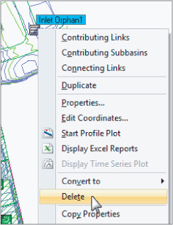
2. With the selection tool active, locate the Inlet named Orphan1.
As you pause your cursor over the various nodes and junctions, the tooltip will tell you which item you are examining.
3. Right-click on Inlet Orphan1 and click Delete, as shown in
Figure 15.52.
4. Click Yes to verify the deletion.
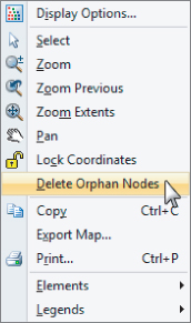
Deleting a single entity will come in handy, but you may find that after import from Civil 3D, you still have many disconnected and unneeded nodes. For this situation, you will use Delete Orphan nodes.
5. To delete the remaining disconnected inlets, right-click anywhere there is not an entity in the drawing and click Delete Orphan Nodes, as shown in
Figure 15.53.
6. Click Yes when prompted to verify.
Next, you will allow for exfiltration from your pond. As water sits, it will leave the pond as it seeps into the ground water below.
7. Double-click Project Options.
a. Verify that the Link Routing method is Hydrodynamic.
b. Change the storage node exfiltration method to Constant Rate, Wetted Area.
This option means that the loss rate changes as a function of the wet surface of the earth that forms the basin.
8. When the project options look like
Figure 15.54, click OK.

9. Click the storage node tool and place a storage node in the graphic in the pond area, south of the outfalls.
10. Press Esc to return to the selection tool.
11. Double-click the new storage node.
a. Change the Storage Node ID to Pond.
b. Set the Invert elevation to 775′ (236.2 m).
c. Set the Maximum elevation to 784 (239.0 m).
d. Change Storage Shape Type to Storage Curve.
e. Set Exfiltration to At All Elevations.
f. Set Exfiltration Rate to 0.04 in/hr (1 mm/hr). This value is the typical exfiltration rate for a silty clay soil.
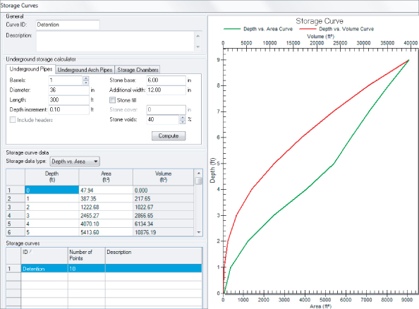
12. Click the ellipsis to the right of the Storage Curve selection. This will open the Storage Curves dialog.
a. Click Add.
b. Rename the Curve ID to Detention.
c. Click Load. Make sure the file type is set to AECCSST.
This is the file you created in Civil 3D when you created a stage-storage table. If you were able to export this file earlier in the chapter, browse to the file you created. If not, use the file Pond-Eval_FINISHED.aeccsst (Pond-Eval_METRIC_FINISHED.aeccsst) provided at the web page.
13. When your storage curve looks like
Figure 15.55, click Close.
14. Verify that the storage curve listed in the Storage Node dialog is set to Detention and click Close.
You will complete the model by connecting the ends of both pipe runs to the storage node. You will need to convert both outfalls to junctions and specify a new outfall.
15. Right-click one of the outfalls and select Convert To ⇒ Junction.
16. Repeat this for the second outfall.
Both outfalls are now junctions. (If time permits, rename the node to reflect that they are now junctions).
17. Before you place the links, be sure to set the invert elevation for the outfall.
Pipes always inherit the invert elevations from the junctions they are connected to.
18. Click the outfall tool and place a new outfall to the south of the storage node.
19. Double-click the new outfall and set its invert elevation to 773′ (235.6 m), then click Close.
20. Start the Add Conveyance Link tool.
21. Working upstream to downstream, connect each junction to the storage node.
22. Double-click one of the conveyance links that connects the junction to the storage node.
23. Set Shape to Direct. Repeat this for the other conveyance link as shown in
Figure 15.56.
Next, you will model an outflow riser using the Orifice tool.

24. Click Add Orifice.
25. Connect the storage node to the final outfall and press Esc.
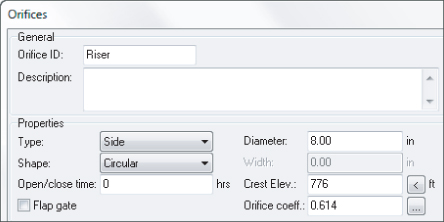
26. Double-click the new Orifice link.
a. Change the Orifice ID to Riser.
b. Set Diameter to 8″ (200 mm).
c. Set the crest elevation to 776′ (236.5 m). This will allow for 1′ (0.3 m) of standing water in the pond.
27. Leave all other options as shown in
Figure 15.57, and click Close.
28. Click Perform Analysis.
If the analysis does not run correctly, review the steps and try again.
29. When the analysis is complete, click OK.
30. Right-click on the orifice and select Display Time Series Plot.
31. Save and close the project.

Stormwater Best Management Practices and EPA SWMM
Stormwater best management practices are intended to remove sediment and other pollutants from drainage systems. Many municipalities require using the EPA SWMM hydrology method to determine the efficacy of these methods.
In the following example, you will walk through how to account for sediment removal at a junction. Again, some important (but time-consuming) tasks have been performed for you already:
The Hydrology method in the Project Options dialog has been set to EPA SWMM.
- The curve number and physical properties of the subbasins have been set.
- A rain gauge indicating an SCS Type II storm has been created and assigned to all subbasins.
1. Open the file Sediment Removal.spf (or Sediment Removal_METRIC.spf), which you can download from this book's web page.
2. From the data tree on the left side of the SSA window, double-click Pollutants.
3. In the Pollutants dialog, click Add.
4. Change Pollutant ID to TSS.
5. In the Description area, type Total Suspended Solids, and click Close.
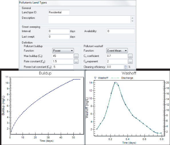
6. Double-click Pollutant Land Types, and click Add.
7. Rename Land Type ID to Residential.
8. Set Pollutant Buildup Function to Power.
9. Set Max Buildup (C1) to 45.
10. Set Rate Constant (C2) to 1.5.
11. Set Power/Sat Constant to 0.5.
12. Set Pollutant Washoff Function to Event Mean.
13. Set C1 Coefficient to 0.7. Set C2 Coefficient to 2.
14. Close the Pollutant Land Types dialog.
15. Double-click the junction named Sediment Removal.
16. Click the ellipsis next to Treatments.
17. In the Treatment Expression column for TSS, type R=0.8.
This expression indicates that 80 percent of TSS is removed by this treatment.
18. Click OK when complete.
19. Close the Junctions dialog.
20. Double-click one of the subbasins to open the Subbasins dialog.
21. Switch to the Flow Properties tab.
22. Click the ellipsis next to the Land Type field.
23. Double-click next to Residential and type 100, and then click OK.
24. Repeat steps 22 and 23 for all of the subbasins.
25. For each subbasin, set 100 percent of the land area to Residential. Click OK after each entry. Close the Subbasins dialog.
This is the pollutant land type you defined in the previous steps.
26. Click Perform Analysis; then click OK. Save and close the project.
You can now show the efficacy of your treatment as it relates to the rest of the storm design.
Running Reports from SSA
There are many places in SSA to view the results of your work. After you've run the analysis, the link and node listing will tell you if your pipe is underdesigned or if there is water backing up in the manholes.

From virtually every dialog in SSA, clicking the Report button will create an Excel spreadsheet from the data you are observing. You will see the Report button for links, nodes, junctions, outfalls, and subbasins.
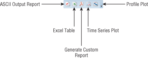
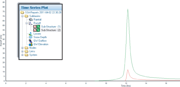
After running the analysis, you will want to see performance information and graphical representations of the relationship between the parts of your design. The Reports toolbar is at the top of the SSA screen. Figure 15.59 shows the different types of reports that you can choose.
First, let's take a look at the hydrograph that has been created for the site:
1. From SSA, open the file SSA-Reports.spf, which you can download from this book's web page.
2. Click the Perform Analysis button. Click OK.
3. Click the Time Series Plot button.
4. On the left side of the screen, expand the Subbasins folder.
5. Click the word Runoff.
A plus sign will appear.
6. Click the plus sign to expand the listing.
7. Put a check mark next to both subbasins, as shown in
Figure 15.60.
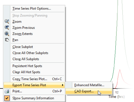
8. Right-click anywhere in the graph area.
9. Select Export Time Series Plot ⇒ CAD Export, as shown in
Figure 15.61.
10. Save the resulting DWG to your desktop as SSA-OUT.dwg.
11. Close the Time Series Plot tab.
Remain in the SSA project for the next exercise.
A common analysis you will want to examine is the profile plot. On the left side of the SSA window you will see the Profile Plot option. Once the profile plot settings appear, you can graphically select the nodes you wish to include in your output.
In the next exercise, you will examine a profile plot for the pipes in the system:
1. From SSA, continue working in SSA-Reports.spf.
You do not need to have completed the previous exercise to continue—you can download this file from the book's web page.
2. Click the Perform Analysis button, and then click OK.
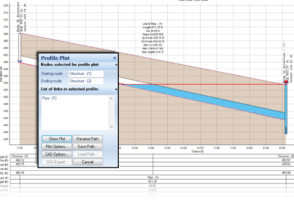
3. From the Reports toolbar, select Profile Plot.
On the left side you can specify Starting Node and Ending Node. You can also specify the link you'd like to plot by clicking on it in the graphic.
4. Click the link Pipe - (1).
The pipe will highlight in the plan view.
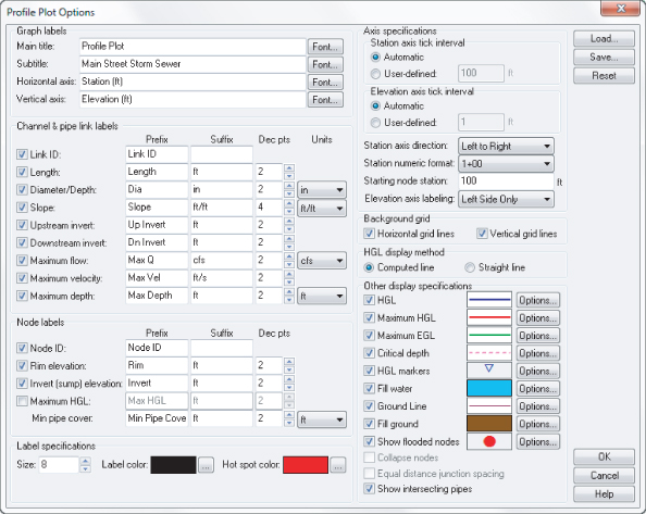
5. Click Plot Options.
6. In the Plot Options dialog, place a check mark next to Maximum Flow, Maximum Velocity, and Maximum Depth.
7. In the Other Display Specifications, place a check mark next to Maximum EGL, Critical Depth, HGL Markers, and Show Flooded Node.
Your Profile Plot Options dialog should resemble
Figure 15.62.
8. Click OK.
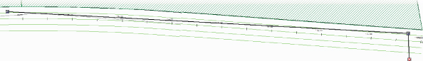
9. Click Show Plot.
Your graphic should resemble Figure 15.63.
After your break from the world of Civil 3D, it is time to export SSA modified data back to CAD. At first glance, you may be thinking that CAD Export or LandXML may be the way to go. However, those options are not the best way to maintain the integrity of your pipe and structure objects. The best option for getting your edits back into Civil 3D is to use File ⇒ Export ⇒ Hydraflow Storm Sewers File.
The following exercise will walk you through the steps needed to get back to Civil 3D:
1. From SSA, open the file SSAtoC3D.spf.
You can download this file from this book's web page.
2. Choose File ⇒ Export ⇒ Hydraflow Storm Sewers File, as shown in
Figure 15.64.
3. Save the file as SSAtoC3D.stm on your computer's desktop.
4. Close SSA.
5. In Civil 3D, open the file C3DtoSSA.dwg.
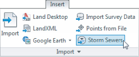
6. From the Import panel on the Insert tab, select Storm Sewers as shown in
Figure 15.65.
7. Browse to the STM file you exported and click Open.
You will get a warning that there is already a pipe network with the same name in the file.
8. Click Update The Existing Pipe Network.
After a moment, your pipes and structures should reflect any size or elevation changes that may have occurred in SSA.
The Bottom Line
Create a catchment object.
Catchment objects are the newest object type that Civil 3D can use to determine the area and time of concentration of a site. You can create a catchment from a surface, but in most cases you will use the option to create from a polyline.
Master It
Create a catchment for predeveloped conditions on the site.
Export pipe data from Civil 3D into SSA.
Civil 3D by itself cannot do pipe flow or runoff calculations. For this reason, it is important to export Civil 3D pipe networks into the Storm And Sanitary Analysis portion of the product.
Master It
Verify your pipe export settings and then export to SSA.
Export a stage-storage table from Civil 3D.
When designing detention basins in Civil 3D, you will often need to export surface data for analysis in SSA.
Master It
Generate a stage storage table for a detention basin surface. Determine how much water the pond can hold.
Model drainage systems in SSA.
SSA is capable of modeling everything from complex drainage systems to simple culverts.
Master It
Determine which links flood during a 2-hour, 50-year storm event. Model the example drainage design using SSA.