
4.4. WHAT ARE WE APPROXIMATING? 53
0 1 2 3 4
0:2
0
0:2
0:4
0:6
x
f
(
x
)
Figure 4.2: A generic function is shown over some global domain.
Consider the function f .x/ D e
x
sin.3x/, plotted in Fig. 4.2. In the vicinity of the point
x D 2, the second-order Taylor series approximation represents the function with some level of
accuracy in some prescribed neighborhood of x D 2, as shown in Fig. 4.3. e linear, first-order
Taylor series approximation is a reasonable representation over yet a smaller window. e zeroth-
order Taylor series allows for no interpolation. en it follows that the neighborhood over which
an element’s interpolation function approximates a known solution with acceptable accuracy will
determine the appropriate element size you want in your discretized domain. erefore, it follows
that you cannot know how to best discretize your domain without knowing what element inter-
polation, i. e., element type, you have chosen. As we will see, how well higher-order derivatives of
these interpolating functions represent the derivatives of the actual solution must be considered
in order to determine the accuracy of the stresses predicted by the numerical model.
4.4 WHAT ARE WE APPROXIMATING?
e primary solution variables in FEA are displacements at discrete grid points we call nodes. A
discrete solution using the finite element method always delivers an approximate overall solution
in the entire domain characterized by
1. maintenance of force equilibrium at all nodes and
2. sacrifice of inter-element force equilibrium in neighboring finite elements that share par-
ticular nodal points.

54 4. IT’S ONLY A MODEL
0 1 2 3 4
2
1:5
1
0:5
0
0:5
1
x
f
(
x
)
f
(
x
)
UIPSEFS 5BZMPS TFSJFT
TUPSEFS 5BZMPS TFSJFT
OEPSEFS 5BZMPS TFSJFT
Figure 4.3: Progressively higher-order truncated Taylor series approximations to an arbitrary function
model the function’s behavior well over progressively larger local neighborhoods.
e displaced configuration of an elastic body is precisely the set of nodal point displace-
ments superposed on the original undeformed configuration. e deformed body acts as an elab-
orate three-dimensional spring that, upon unloading, would return instantaneously to its original
size and shape. e set of nodal point displacements comprise a set of coefficients that each mul-
tiply basis functions whose collected weighted sum represents an approximation of the continu-
ous displacement field in three dimensions. Finite element analysis is, in one sense, a piecewise
Lagrange polynomial interpolation of this continuous field into many lower-order polynomials
whose continuity requirements at nodal points are dictated by the order of truncation of the local
Taylor series. It is, therefore, the order of the interpolation or shape function that dictates the
variation of displacement along the interior of the finite element.
Now let’s consider an idealized finite element analysis as an example of:
1. developing and solving a mathematical model,
2. showcasing where particular errors made in finite element practice might occur, and
3. illustrating where theory embedded in finite element formulations is no guarantee that using
finite element analysis will result in an accurate simulation.
4.4. WHAT ARE WE APPROXIMATING? 55
SimCafe Tutorial 5: Four-Point Bend Test on a T-Beam
e purpose of this case study is to showcase how the manner in which boundary
conditions are applied can change with the number of dimensions in the analysis. Prescription
of a single unique “appropriate” set of boundary conditions may no longer exist in a three-
dimensional model vs. its one-dimensional analog. In the case study described here, multiple
prescriptions of a “simple support” lead to significantly different predicted bending stresses
even in the fairly benign circumstances encountered in a four-point bend test.
Follow the directions at https://confluence.cornell.edu/display/
SIMULATION/T-Beam to complete the tutorial.
Example 4.1: Four-Point Bend Test on a T-Beam
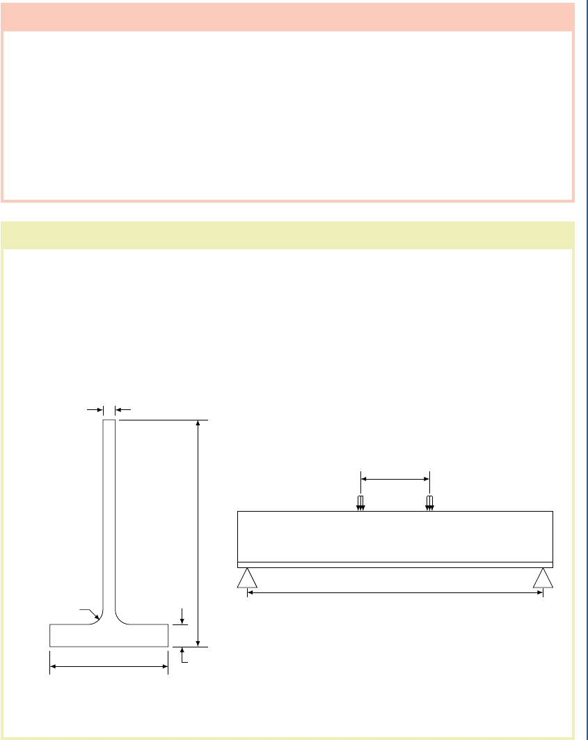
Consider that we are examining a long, slender T-beam loaded at two symmetric loca-
tions on its top surface while being simply supported at its ends along triangular knife-edge
supports as shown in Figs. 4.4 and 4.5. e load was applied with a hydraulic cylinder ap-
paratus. Strain gages mounted at several locations between the loading points (where the
moment was constant and the transverse shear force was zero) were monitored during the
test. We know that the beam is made of isotropic steel with a span of 30 in and constant
cross-sectional properties. We wish to accurately predict its peak bending stress.
3 JO
0:3125 JO
30 JO
P P
7 JO
4ZNNFUSJD MPBET P
BQQMJFE PWFS JO MFOHUI
5:75 JO
0:5625 JO
0:375 JO
Figure 4.4: A T-section beam cross section is pictured, along with a schematic of the loads ap-
plied in a four-point bend test.
I

56 4. IT’S ONLY A MODEL
Example 4.1: Four-Point Bend Test on a T-Beam (continued)
Figure 4.5: e T-section beam is simply supported along triangular knife edges at each end.
We assume the load is quasi-static. e material remains in the elastic range, the beam
is long and slender enough for Euler-Bernoulli beam theory to be a sufficient representation
of the deformation and internal stress response. We neglect contributions to the deformation
from shear deflection. We assume the vertical transverse loads from the hydraulic press can
be modeled as pressures over small contact patches. We also assume the simple support at
the ends of the beam constrain the transverse displacements at the beam’s bottom flange in
contact with the knife-edge support.
Having chosen a one-dimensional beam element, we are assuming a cubic interpola-
tion of transverse deflection between node points to represent a global solution that is cubic.
One would then expect to generate exact results [Irons and Shrive, 1983] as there are no trun-
cation errors in the approximation. A linear distribution of normal, bending stress through
the depth of the section would then be the expected result. e simplest discretization is
shown in Fig. 4.6.
Figure 4.6: A one-dimensional finite element mesh using beam elements is loaded with idealized
point loads.
Comparisons of the normal bending stress results of the one-dimensional analyses
with those determined from strain gage test data from the lab allowed for some interesting
comparisons, as shown in Table 4.1. Here we report the stresses in dimensionless form where
I

4.4. WHAT ARE WE APPROXIMATING? 57
Example 4.1: Four-Point Bend Test on a T-Beam (continued)
the actual stress is normalized with respect to the characteristic bending stress
O D
PLh
2I
:
is illustrates a further point about the finite element method. It is entirely devoid
of any reference to the chosen system of units. ese are entirely at the discretion of the
user. One need only prescribe a consistent set of units in order to interpret results meaning-
fully. Because the units are discretionary, results from linear static analyses scale linearly with
load and dimensionless results are rendered independent of the actual specific load, section
properties, or material constants chosen.
Table 4.1: Results of one-dimensional beam analyses
bottom
= O
top
= O
Experiment 0.1108 -0.2464
Euler-Bernoulli beam theory 0.1134 -0.2724
FEA: beam elements 0.1134 -0.2724
Based on these results, in which physical experiment, simple beam theory, and finite
element simulation are in good agreement, we could conclude that we have obtained an
accurate answer for the peak bending stresses in the beam, and in particular, that the use of
beam elements is an appropriate choice for the finite element model. We further comment
that the alert reader should surmise that the peak stresses occur at the midpoint (x D 15 in).
Recall that models are approximations of reality, and it is quite possible that more than
one model is capable of producing an accurate result. It is well worth asking if a fully three-
dimensional analysis would also verify these results. is may, in fact, be what one expects at
first glance.
To investigate this question, a three-dimensional model is created in which the hy-
draulic loads are approximated as pressure loads over the small contact areas. We also assume
that the knife-edge supports at the left and right ends can be modeled by constraining the
transverse (z-direction) and out-of-plane (y-direction) displacements at all points along left
and right edges of the beam’s bottom flange (that is, along the edge lines parallel to the
y-direction), as shown in Fig. 4.7.
I
..................Content has been hidden....................
You can't read the all page of ebook, please click here login for view all page.