
Appendix B
Influence Diagrams
B.1 Introduction
The purpose of this appendix is to provide an introduction to influence diagrams (ID) and pointers to some of the foundational references. An influence diagram is a compact graphical representation of a decision. Howard and Matheson published the seminal paper on influence diagrams in 1980. The paper was republished in Decision Analysis to be more broadly available (Howard & Matheson, 2005). They developed influence diagrams as a decision problem representation that could be understood by both computers and people. Currently, Howard (Howard, 2004) uses the term “relevance diagram” to describe an influence diagram that contains only uncertainties and “decision diagram” for one that also includes decisions and values. Howard prefers “relevance” to “influence” since an arrow in an ID means that knowledge of one uncertain event is relevant to knowledge of a second uncertain event and not that one event “influences” the outcome of another event.
Shachter developed computation algorithms for influence diagrams that are equivalent to the decision tree algorithm (Shachter, 1986, and Shachter, 1988). This research put influence diagrams on a sound theoretical foundation. Influence diagrams were originally developed for decisions having a single value measure. Merkhofer (Merkhofer, 1990) demonstrated the use of influence diagrams for multiple objective decision analysis.
Influence diagrams are often used in decision analysis textbooks (e.g., Clemen & Reilly, 2001) and decision analysis software is available to solve influence diagrams, producing the same results as the decision tree algorithm (Buckshaw, 2010). Influence diagrams are an important tool for DA practitioners to define the decision frame, identify the variables and decisions that should be included in the decision model, and communicate the structure of the decision model to decision makers and stakeholders (Buede, 2005).
B.2 Influence Diagram Elements
Although an influence diagram may appear to be just an informal “boxes and arrows” drawing, there are precise rules for constructing influence diagrams, which represent N-dimensional probability distributions. The shapes in an influence diagram have specific meanings, and there are a few rules that must be obeyed when drawing an influence diagram. The influence diagram elements are shown in Figure B.1 using common symbols.1
FIGURE B.1 Elements of an influence diagram.
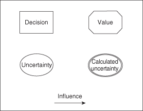
A rectangle represents a decision, which is specified by a set of alternatives. Depending on its purpose, an influence diagram may contain only one rectangle representing a high-level strategic decision, which comprises a set of choices of lower-level decisions, or it may contain several different rectangles each representing a sequence of lower-level decisions. If some decisions are made initially and others are made after some uncertainties are resolved, it is essential to show those decisions as separate nodes in an influence diagram.
An oval represents an uncertainty. Uncertainties differ in two dimensions: (1) continuous versus discrete and (2) scalar versus vector.
An uncertainty may be either continuous or discrete. A continuous uncertainty is a random variable whose value can be any real number in a specified range of outcomes. An example of a continuous uncertainty would be the weight of an object. A continuous uncertainty is specified completely by a continuous probability distribution, such as the normal distribution, but is often characterized by a discrete approximation, usually with only three possible values—low, base, and high.
A discrete uncertainty is a random variable whose value can be any of a specified countable subset of the real numbers, such as the set of integers in a given range. An example of a discrete uncertainty is the number of successful product launches in a given time period. An important type of discrete uncertainty is a binary event, which may either occur or not occur.
An uncertainty may be either scalar or vector. A scalar uncertainty is one described by just a single number. All three examples given above are scalar uncertainties—the weight of an object, the number of product launches, and the occurrence of an event. Often, however, a vector of numbers can also describe an uncertain factor, usually as a time series of values, such as the market share of a product as it changes over time. Each element of the vector might be either continuous or discrete. Uncertainty about the entire vector can be represented by a single oval in the diagram, unless some elements of the vector are known at the time of a decision while others remain uncertain.
A double oval represents a special case of an uncertainty called a calculated or determined uncertainty. This is a factor that is uncertain only because it is calculated from other factors that are uncertain (e.g., the sum of uncertain factors). If each of those other factors were known for sure, the factor represented by the double oval would also be known for sure.
An octagon represents a value measure. The value measure is a decision criterion—a quantity to be maximized (or minimized) by the choice of decision alternative. For example, in most business decisions, the net present value of future cash flows is a value measure.
An arrow represents a relationship between two elements of the decision. The nature of the relationship depends on the types of elements connected by the arrow
Figure B.2 shows the four types of relationships. An arrow between two uncertainties means that there is probabilistic dependence between the two. Note that the absence of an arrow between two uncertainties is actually a stronger assertion—that there is no probabilistic dependence between the two. In other words, knowledge of the outcome of uncertainty A does not provide information about the probability of the outcome of B. The direction of the arrow indicates the order of conditionality. The probabilities of the uncertainty at the head of the arrow are conditional on the outcome of the other uncertainty. The arrow represents an informational relationship and does not necessarily imply causality. For example, an arrow might be drawn from an uncertainty about whether people are carrying umbrellas to an uncertainty about whether it is raining. Such a diagram indicates that observing people carrying umbrellas might affect the probability we assign to rain, but it would not be valid to say that rain is caused by people carrying umbrellas.
FIGURE B.2 Types of influences.
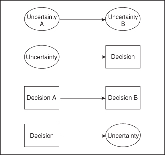
An arrow from an uncertainty to a decision means that the outcome of the uncertainty is known when the decision is made. This arrow represents a strong assertion about timing—that the resolution of the uncertainty occurs before the decision is made.
An arrow between two decisions means that when the decision at the head of the arrow is made, the choice taken in the other decision is remembered perfectly. This “no forgetting” arrow makes a strong assertion about the relative timing of the two decisions.
Finally, an arrow from a decision to an uncertainty means that the probabilities for the uncertainty depend on the choice made in the decision. Such an arrow is often used to describe a situation in which an uncertain outcome is revealed only if a particular action is taken. For example, the decision might be whether or not to do a diagnostic test and the associated uncertainty would be the result of that test with three possible outcomes—good result, bad result, or no result. Clearly, the probabilities for these outcomes depend on the choice made in the decision, because the probability of no result is 100% if the test is not done, whereas it is 0% if the test is done.
Drawing an influence diagram with an arrow from a decision to an uncertainty places a severe restriction on the decision situation so described—it may be impossible to calculate the value of clairvoyance (perfect information) on that uncertainty. It is always possible to modify such an influence diagram by adding calculated uncertainties so that the diagram has no arrows from decisions to uncertainties, as illustrated in Figure B.3. An influence diagram in which no arrow exists from a decision to an uncertainty is said to be in Howard canonical form.
FIGURE B.3 Probabilities conditional on a decision (left) and Howard canonical form (right).

B.3 Influence Diagram Rules
There are three important influence diagram rules, one of which (Rule 1) must be obeyed for all influence diagrams.
B.3.1 RULE 1: NO LOOPS
There must not be any path in the diagram that forms a directed loop. That is, it must always be impossible to return to any element in the diagram by following arrows in the direction that they point. Violation of this rule invalidates the underlying mathematical foundation of the diagram and creates a situation in which it could be impossible to assess probabilities for all of the uncertainties.
Two additional rules must be obeyed if the influence diagram is to describe a situation that can also be represented by a decision tree.
B.3.2 RULE 2: ONE VALUE MEASURE
All decisions represented in the diagram must be made to optimize the same value measure. However, multiple value nodes can be used to calculate one value measure.
B.3.3 RULE 3: NO FORGETTING
Any information known when a decision is made must be remembered perfectly when any subsequent decision is made. This implies that between every pair of decisions in an influence diagram, there must be a directed path that includes only decision nodes. And, if there is an arrow from an uncertainty to a decision, there must also be an arrow from that uncertainty to any subsequent decision.2
B.4 SUMMARY
This appendix provides an introduction to influence diagrams and pointers to some of the foundational references. Influence diagrams are an important tool for DA practitioners to define the decision frame, identify the variables and decisions that should be included in the decision model, and communicate the structure of the decision model to decision makers and stakeholders. Decision analysis software is available to solve influence diagrams that provide the same results as the decision tree algorithm.
Notes
1Different software uses different symbols.
2Some influence diagram software, for example, DPL, does not require these arrows to be in the influence diagram, since the sequence is specified in the decision tree window.
REFERENCES
Buckshaw, D. (2010). ORMS Today. Retrieved December 17, 2011, from Decision Analysis Survey, http://www.orms-today.org/surveys/das/das.html.
Buede, D.M. (2005). Influence diagrams: A practitioners perspective. Decision Analysis, 2(4), 235–237.
Clemen, R.T. & Reilly, T. (2001). Making Hard Choices with Decision Tools. Duxbury.
Howard, R.A. (2004). Speaking of decisions: Precise decision language. Decision Analysis, 1(2), 71–78.
Howard, R.A. & Matheson, J.A. (2005). Influence diagrams. Decision Analysis, 2(3), 127–143.
Merkhofer, M.M. (1990). Using influence diagram in multiattribute utility analysis: Improving effectiveness through improved communications. In R.M. Oliver & J.Q. Smith (eds.), Influence Diagrams, Belief Nets, and Decision Analysis, pp. 297–316. John Wiley & Sons.
Shachter, R.D. (1986). Evaluating influence diagrams. Operations Research, 34, 871–882.
Shachter, R.D. (1988). Probabalistic inference and influence diagrams. Operations Research, 36, 589–605.