CHAPTER ELEVEN

Perform Probabilistic Analysis and Identify Insights

ERIC R. JOHNSON and STEVEN N. TANI

An organization’s ability to learn, and translate that learning into action rapidly, is the ultimate competitive advantage.

—Jack Welch

11.1 Introduction

Previous chapters discuss initial development of a composite perspective on what drives value for the decision. To improve and exploit the composite perspective, we must find ways to understand the behavior of value that emerges from this model and test these against individuals’ perspectives. For decisions involving significant uncertainty, explicitly modeling uncertainty with probability gives us an improved perspective on the value and risk of the alternatives. This is a key part of the learning that Jack Welch emphasizes in our headline quote. This chapter shows how to achieve that learning and use it to improve the value and/or mitigate the risk of the recommended alternative(s).

The chapter is organized as follows. Section 11.2 presents the two main ways to incorporate uncertainty in our decision model: decision trees and simulation. Both approaches can create complex emergent behavior that manifests itself across all the other dimensions. Section 11.3 shows how to generate comprehensible analyses that facilitate critical comparison of perspectives and development of improved strategies. We refer to this process as a value dialogue. Section 11.4 is a discussion of how to incorporate risk attitude in a decision analysis when appropriate. Our Roughneck North American Strategy (RNAS) illustrative example (introduced in Chapter 1) is referenced throughout the chapter. Section 11.5 reviews how probabilistic analysis was done in the other two illustrative examples, and the chapter is summarized in Section 11.6.

It is important to note that all the techniques described in this chapter can be applied to single- and multiple-objective decision analysis. The examples we use are single-objective decision analyses. See Parnell et al. (2011) for examples of multiobjective decision analysis (MODA) with Monte Carlo simulation and decision trees.

Some people may feel that the purpose of decision analysis is to make the right choice among a given set of options, and view the development of even better courses of action as an optional activity. While the relative amount of value created by these two activities varies widely, depending on the situation, simply making the right choice from the initial set of options can leave substantial value on the table, particularly if none of the original options satisfies the fundamental objectives very well. Hence, this chapter aims to support strategy improvement as well as identification of the optimal choice among the initial set of strategies.

This chapter and Chapter 13 both discuss communication with stakeholders, but the spirit of the communication in the two is different. Here, value implications of the composite perspective are communicated in the spirit of critical inquiry; Chapter 13 discusses communication of a chosen strategy in the spirit of building understanding of insights that support decision making and commitment to action.

Much of the discussion here is framed as finding or adding value. The other side of this coin is identifying and mitigating risk. While these have different connotations, approaches discussed in this chapter are equally applicable to both: create a composite perspective, understand what drives value and risk, and hypothesize and test strategies that may achieve higher value and/or reduce risk.

11.2 Exploration of Uncertainty: Decision Trees and Simulation

As discussed previously, our recommended tool to identify the uncertain variables and their probabilistic interactions is the influence diagram (see Chapter 10 and Appendix B). As discussed in Chapter 9, the two ways to represent uncertainty are extensive (representing all possible combinations simultaneously) and intensive (representing one combination at a time). For an extensive decision tree representation of uncertainty, the method of analysis is to roll back the tree (see Section 11.2.1). For an intensive representation in an Excel model, the choice of analytic method is between decision trees and simulation.

11.2.1 DECISION TREES

A decision tree (Luce & Raiffa, 1957) is an extensive representation of all possible outcomes of uncertainty. In a decision tree, each possible outcome is depicted by a path through a tree. Conventionally, trees flow rightward from a point of origin (“root”) at the left, with a branching point (“node”) for each uncertainty and decision. Uncertainty nodes are conventionally shown as circles, and branches emerging from them are possible outcomes. The conditional probability of each outcome is noted on the branch. A decision node is shown as a square, and branches to its right represent possible choices for that decision. Decisions are arranged chronologically with earliest at the left and latest at the right. Uncertainties to the left of a decision must be resolved by the time the decision is made, so each decision node represents a decision in a distinct state of information. The value of an outcome corresponding to a particular path through the tree (a “scenario”) is shown at the far right end of the path (the “leaves” of the tree).

The optimal choice and its value at each decision node can be calculated using a rollback procedure (Raiffa, 1968). In it, we start at the right and calculate the value at each node in turn. If it is an uncertainty, we substitute a leaf whose value is the EV (expected value) of the branches for that subtree. If the node is a decision, we note which alternative gives the best value in that circumstance, and substitute the value of the optimal choice for the subtree. This process continues until the entire tree has been simplified to a leaf, indicating the value of the optimal set of choices, and the optimal choices in all states of information have been noted.

Software packages are available to process an intensive representation of uncertainty and alternatives in decision tree fashion. These packages make it easy to specify the structure of the tree, including conditional probabilities. Typically, these packages cache and aggregate only a single value metric; some can handle multiple value measures in the rollback. The size of a tree, and the computational time to evaluate it, rises geometrically with the number of uncertainties included, so the tree should contain only the most important uncertainties. We use tornado diagrams, as explained in Section 9.8.2, to identify which uncertainties to put into the tree.

Another interesting use of trees is for game theory situations. In game theory, we consider multiple rational decision makers (“players”) in a situation where the actions of each player influence the outcomes of the others. Formulating such models requires attention to the states of information of the participants when they make their decisions, and the solution approach or software must ascertain the value realized by each player in each scenario. The notion of what behavior is optimal is more complex in a game theory situation. The most common insight from game theoretic analysis is that delivery of a credible threat can sometimes influence the behavior of another player in ways favorable to oneself. Discussion of game theory is beyond the scope of this handbook. See Papayoanou (2010) for a recent practitioner’s treatment, and Bueno de Mesquita (2002) for a discussion of recent game theoretic view of American foreign policy.

11.2.1.1 Example Decision Tree Application. 

To see how a decision tree can be used to resolve an important decision situation, consider the example of a company planning to build a manufacturing plant for a new product due to be launched in2 years. We find it helpful to develop an influence diagram such as the one shown in Figure 11.1 as the first step in developing the decision tree.

FIGURE 11.1 Influence diagram for capacity planning example.

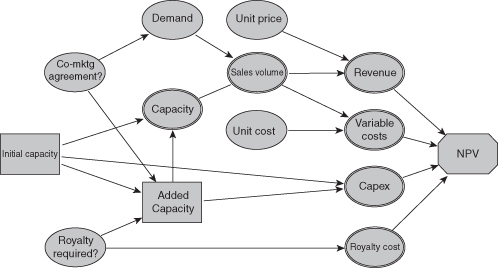
The key decision under consideration is how much capacity to build into the new plant. This decision is made difficult by several sources of uncertainty. The future level of demand for the new product is quite uncertain, ranging from a low (10th percentile) of 200K units per year to a high (90th percentile) of 1000K units per year, and is made even more uncertain by the possibility that a comarketing agreement will be signed with a TV cable channel that would boost demand substantially (by about 40%). And the degree of profitability of the product is uncertain because of uncertainty in both unit cost and selling price, as well as the chance that a pending patent infringement lawsuit will be lost, requiring that a royalty be paid on all sales of the product.

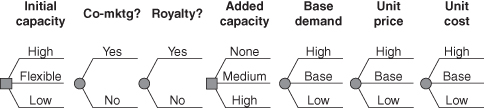
The decision team plans to build out capacity in two stages. The initial level of capacity must be chosen now, but capacity can be expanded 4 years from now. Capacity installed initially has a lower per-unit cost than capacity added later. But waiting to add capacity has the advantage that two key uncertainties will be resolved by the time that decision is made—whether the comarketing agreement is signed and whether the patent infringement lawsuit is won or lost. For initial capacity, the team has identified three alternatives:

For the capacity expansion 4 years from now, the team has chosen three levels to analyze:

Clearly, the optimal amount of capacity to add will be driven by how much capacity was built initially, the demand forecast (given whether or not the co-marketing agreement has been signed), the cost of adding capacity (given whether the Flexible alternative was chosen initially), and the projected profitability of the product (given whether or not a royalty will be required). Because of this “downstream” decision, a decision tree approach is the best way to analyze the situation.

The decision tree for the capacity planning decision is illustrated schematically in Figure 11.2.

FIGURE 11.2 Schematic decision tree for capacity planning example.

This decision tree has 972 unique paths and is small relative to many trees developed in professional practice, which can have many thousands of paths. But it is sufficient to provide good decision insight in this situation.

To evaluate the tree, a spreadsheet model is built to calculate the net present value (NPV) for the product for each path through the tree (scenario). This model is then connected to decision tree software, which performs the rollback calculations. The results of the rollback are shown in the partial tree display in Figure 11.3.

FIGURE 11.3 Partial display of evaluated decision tree for capacity planning example (values in $ million).

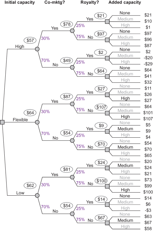
Each of the 36 NPVs at the right-hand end of the partial tree is the expected value of 27 NPVs for different combinations of demand, unit cost, and selling price. We can see from the tree that the optimal decision policy is to choose the Flexible alternative for initial capacity and then to choose high added capacity if the comarketing agreement is signed and medium added capacity if it is not. The optimal policy has an expected NPV of $64 versus $62 million for starting with low initial capacity and $57 million for starting with High initial capacity.

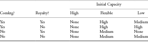
Note that the optimal choices for the downstream decision may not be easy to predict intuitively (see Table 11.1).

TABLE 11.1 Optimal Downstream Decisions in Capacity Planning Example

11.2.2 SIMULATION

We refer to a particular combination of outcomes of all uncertainties as a scenario. In a simulation approach, we sample repeatedly from possible scenarios with probability distributions driven by the composite perspective and record the aggregated results. A description of marginal and conditional probabilities in an influence diagram (see Fig. 10.2 in Chapter 10) and encoded in an Input sheet of a spreadsheet (see Fig. 9.2 in Chapter 9) is an intensive representation of the composite perspective. Chapter 9 discusses construction of a spreadsheet model that embodies this representation in a form that can be manipulated.

Simulation is viewed as a sub-discipline of operations research, and it can play an important role in decision analysis. Different kinds of simulation have been developed, indicating different areas of emphasis:

• Monte Carlo simulation. Realization of a sequence of outcomes by repeated random sampling of input scenarios according to probability distributions. In decision analysis, we obtain these distributions from experts.
• System dynamics. Simulation of flow through a network of transformations over time, typically focusing on the implications of positive or negative feedback loops in the network (Forrester, 1961).
• Agent-based simulation. Simulation of the behavior of a community of interacting “agents” or actors, each of which has objectives and a behavioral repertoire represented by deterministic or probabilistic rules.
• Discrete-event simulation. Simulation of a system that is represented as a chronological sequence of events. Each event occurs at an instant in time and marks a change of state in the system (Robinson, 2004).

When the term “simulation” is used in this handbook, we have in mind Monte Carlo simulation, but other variants of simulation should be employed if appropriate for the situation at hand.

The normal way to aggregate value across simulated scenarios is to calculate the expected value (EV), because this is the required way to handle utility, and it is frequently informative for other value measures. Calculation of EVs requires caching and aggregation (or on-the-fly aggregation) of the instantiated values. Commercially available simulation packages support caching and aggregation of a large number of value measures.

One characteristic of Monte Carlo simulation is that it introduces a certain amount of noise into results. This can be managed by choosing an adequate number of iterations, or “trials.” In practice, the number of trials required is not strongly influenced by the number of uncertain variables. If there are rare events with important consequences, a standard Monte Carlo will require a larger number of trials to give reliable results. Variants, such as importance sampling (Asmussen & Glynn, 2007), can be employed in such cases.

11.2.2.1 Monte Carlo Sampling. 

In Monte Carlo simulation, it is important to select a sampling distribution for each uncertain parameter that fairly represents the impact of plausible extremes (10th percentile, denoted “P10,” and 90th percentile, denoted “P90”), as well as the central tendency of value. But it may not be important for the cumulative distribution curve of a sampling distribution to look plausible. For instance, for many intrinsically continuous uncertainties, a three-point discretization (which has a stairstep cumulative probability curve) is often adequate. We discuss a few reasonable sampling distributions here, but others will suffice.

A good and simple approach is to use a discrete sampling distribution that gives 30/40/30 probabilities to the expert’s P10-50-90 inputs. This “extended Swanson–Megill” distribution preserves the mean and variance of a variety of utility functions (Keefer, 1994). Some people prefer 25/50/25 probabilities. While this is apt to understate the variance of the resulting distribution of value, the understatement may not be large, so this is also a good choice.

For a variable that we may want to use as a precondition for a future decision, it can be important that the sampling distribution gives some nonzero probability density over a range of values (i.e., a continuous support). For these cases, the most authentic representation is to elicit a full continuous distribution from the expert, but this can be time consuming, especially if there are multiple experts. Often we can develop the insights we need by fitting a continuous curve to the P10-50-90 assessment we have and using it as a sampling distribution. Various distributions, including the skew logistic (Lindley, 1987) or a distribution we call the Brown–Johnson, can be used in this way. Brown–Johnson is piecewise uniform in the four ranges, from its P0 to P10 to P50 to P90 to P100.¹

For example, in the Roughneck North American Strategy (RNAS) illustrative example (see Section 1.5.1 for the case introduction), the model makes extensive use of 30/40/30 probabilities of P10-50-90s. However, a continuous distribution on future oil price is needed to test various levels of the go-forward threshold for Tar Sands full-scale development. The analysis uses a Brown-Johnson distribution for oil price based on carefully assessed P10-50-90 points.

11.2.2.2 Cumulative Probabilities and Uncertainties. 

Generation of an EV tornado diagram using the approach described later in this chapter (see Section 11.3.4) requires the cumulative probability at which each uncertainty is sampled for each trial. One way to provide this is to generate the cumulative probability first by sampling from a Uniform[0,1], and then to calculate the corresponding fractile within its sampling distribution. This is straightforward for both extended Swanson–Megill and Brown–Johnson, as shown in Figure 11.4.

FIGURE 11.4 Extended Swanson–Megill and Brown–Johnson distributions.

Typically in Monte Carlo simulation, a distinct sample is generated for each uncertainty in each iteration/trial. In cases where experts believe that two or more variables are strongly linked (e.g., by specifying the same “Factors Making It High” for those variables in the assessment interview), these variables should use the same sampled cumulative probability in each trial of the simulation. In such a case, it is helpful and usually straightforward to find a name for the common sample that reflects this use. For instance, in the RNAS model, the sample named CBM Cost is used for six variables, relating to CBM opex and capex under various strategies. The CBM Cost bar in the tornado diagram represents the combined impact of all six variables moving in concert.

If we are simply comparing EV results from different strategies, it does not matter whether the same samples are used across all strategies. However, for delta EV tornado diagrams (see Section 11.3.5), if the experts believe that a variable’s outcome is unaffected by strategy choice, the same sample can be used for simulating the variable under all strategies. This constitutes perfect correlation across strategies, and is reasonable if the same Factors Making It High apply across all strategies. If the Factors Making It High are different from one strategy to the next, independent samples should be used, indicating that these variables are independent. If a target variable has been specified using probabilistic conditioning, samples should be drawn from the distribution that is appropriate for the predecessor’s value. Some of the Monte Carlo software packages support the specification of probabilistic conditioning on input variables.

11.2.2.3 Running a Simulation Model. 

Having built the model and set up the sampling logic, the next step is to run a simulation. If strategies are also specified intensively, this requires defining strategies, specifying overrides (if any), and specifying the number of strategies and trials per strategy.

Override values are values for one or more uncertainties to be used in all trials, regardless of the sampling distribution.

Strategies are specified in a strategy table data structure. Initially, the strategies generated in the structuring workshop are tested. As hybrid strategies are developed, these can also be specified and simulated. If we are testing for the optimal parameter for a decision rule, we can specify a number of strategies all identical except for the decision rule parameter. For instance, for RNAS Tar Sands, we specified various oil price thresholds below which the full-scale plant would not be built and compared their results. In addition, when we want to map out an efficient frontier for portfolio analysis, it can be useful to formulate and simulate stylized strategies that test each possible level of investment at each business unit. By doing this, we can then use the results to calculate the incremental cash flow for each opportunity.

Selecting the number of trials to run in a Monte Carlo simulation gives us control over the amount of simulation noise introduced into the results. If we run a simulation with sufficiently many trials, the size of this simulation error can be made small enough that it does not interfere with the critical comparison and exploration required to develop insights and make decisions. But runtime increases if we run more trials, so this runtime–precision trade-off must be managed.

One must understand how much simulation noise is present to avoid overinterpreting noise. While the mathematics of simulation variances is beyond our scope, one key fact to bear in mind is that noise is reduced by the square root of the number of trials. Running four times as many trials cuts noise in half. Running nine times as many trials cuts noise to one-third. It can be helpful to employ one or more dummy variables in the model to understand the impact of simulation noise on EV tornado diagrams. A dummy variable is a variable with a sampling distribution, but with no impact on the calculation. The true width of its tornado bar, if a sufficiently large number of trials were employed, would be zero. This means that any observed variation of value attributable solely to a dummy variable in the tornado is simulation noise. If a variable’s tornado bar is narrower than that of a dummy variable, there is no reason to think that uncertainty in such a variable has a material impact on uncertainty in value. If this creates difficulty, run more trials.

11.2.3 CHOOSING BETWEEN MONTE CARLO SIMULATION AND DECISION TREES

Monte Carlo simulation and decision trees are two different methods to solve the same problem—given a number (N) of important uncertain inputs, find the probability distribution on the value metric for each decision alternative. Both methods accomplish this by examining points in the N-dimensional space defined by the N uncertainties. The methods differ in the way those points are selected. In Monte Carlo simulation, the points are selected “randomly,”² based on the probability distributions of the inputs. In the decision tree method, the points to be examined are preselected as every possible combination of the values of the discrete inputs.

When done well, both methods produce comparable results. However, there are some characteristics of the decision situation that may influence the choice of method.

11.2.3.1 Downstream Decisions. 

The decision tree method is better suited than the Monte Carlo method to handle downstream decisions (i.e., decisions that will be made in the future after some uncertainty is resolved). An important class of decision situations with this characteristic is called “real options.” As illustrated in the capacity planning example (Section 11.2.1.1), the decision tree method handles downstream decisions “automatically” by determining in the rollback procedure the optimal choice for each such decision in the tree. To handle downstream decisions in the Monte Carlo method, a side analysis must be conducted to determine the optimal choices for the downstream decision given each possible conditioning scenario. These optimal downstream choices must then be “hardwired” into the simulation analysis of the original decision alternatives. (This approach is illustrated for the RNAS Tar Sands decision in Section 11.3.8.)

11.2.3.2 Number of Uncertainties. 

The number of uncertain inputs to be included in the probabilistic analysis can push the choice toward either method, depending on whether the number is small or large.

If the number of uncertain inputs is small (say, fewer than eight), the decision tree method is computationally better than Monte Carlo. Consider a case in which there are just five important uncertain inputs. Assuming that each input is discretized with three possible settings, the total number of unique scenarios to be examined is 243 (= 3⁵). Because the decision tree method examines each scenario only once, it would require only 243 evaluations of the value function. But if the analysis were done with Monte Carlo simulation using only 243 trials, there is no guarantee (and very little likelihood) that each of the 243 scenarios would be examined. In fact, a great many more trials need to be run in the Monte Carlo simulation for the probability of each scenario to be accurately portrayed. So, with a small number of uncertainties, the decision tree method is more efficient in computational time than Monte Carlo.

However, if the number of uncertain inputs is large (say, more than 11), then the Monte Carlo method is computationally better than decision trees. The decision tree method requires that every possible scenario be examined. So, for example, in an analysis having 12 uncertain inputs (each discretized with three possible settings), the decision tree method would need to evaluate the value function for over a half million scenarios, requiring substantial computational time. By contrast, the Monte Carlo method allows the analyst to make an explicit trade-off between running time and accuracy of results by choosing the number of simulation trials. Of course, the analyst should avoid the delusion that running a Monte Carlo simulation with just a few thousand trials always produces valid results. Instead, the analyst should monitor the mean square error (MSE) statistic produced by most Monte Carlo software packages to gauge whether the number of trials is sufficient.

What if there are many uncertain inputs defined for a decision but not all of them are really important contributors to overall uncertainty in value? In this case, the Monte Carlo method often gets the nod because of ease of use. With the decision tree method, one would need to produce a tornado diagram to identify the most important uncertainties and then specify those to the decision tree software. With Monte Carlo, one could simply include all uncertainties in the simulation. The important uncertainties are sure to be included, and the fact that many unimportant uncertainties are included does not matter.

11.2.3.3 Anomalies in the Value Function. 

If the value metric is smooth and “well-behaved” over the range of possible input settings, then discrete approximations can be made for all of the inputs in the probabilistic analysis and the results will be quite close to those that would be produced using continuous distributions on the inputs (assuming that there are more than a few inputs with a material impact). However, if there are anomalies in the value function, then discrete approximations are not appropriate and the Monte Carlo method using continuous input distributions is a much better choice than the decision tree method. An anomaly exists if, for some region in the N-space of inputs, the value metric changes rapidly for small changes in the inputs (i.e., a “sink hole” or “pinnacle”). An example of a decision situation with a value function anomaly is a company making choices that could lead to illiquidity. For a setting of inputs that define a scenario in which the company is close to having insufficient cash balances, a small change in inputs could result in a big and disastrous impact—insolvency and shutdown.

It is a wise decision analyst who has both Monte Carlo and decision trees in his or her tool bag. As described above, depending on the situation, one or the other method may be much preferred. And for the situations when either method will serve well, the choice can be made based on the analyst’s preferences and familiarity with the software tools.

11.2.4 SOFTWARE FOR SIMULATION AND DECISION TREES

Software packages are available to process an Excel model in either decision tree or simulation fashion. The professional society INFORMS periodically publishes a thorough review of DA software (http://www.informs.org/ORMS-Today/Public-Articles/October-Volume-37-Number-5/Decision-Analysis-Software-Survey). Software used for the illustrative examples reported in this book includes Excel with VBA, Analytica^® (Lumina Decision Systems, Los Gatos, CA; http://www.lumina.com), and @Risk (Palisade Corporation, Ithaca, NY; http://www.palisade.com/decisiontools_suite) for RNAS; Excel and Crystal Ball (Oracle Corporation, Redwood Shores, CA; http://www.oracle.com/us/products/applications/crystalball/index.html) for data center; and Excel for Geneptin Personalized Medicine.

Some decision analysis software offers the capability to model with influence diagrams and/or decision trees and then, if the computational time is too long, to solve with Monte Carlo simulation.

An additional feature of some influence diagram, Bayesian net, and decision tree software is automatic Bayesian calculations. In this software, the user inputs marginal and conditional probabilities for one order of conditioning, and the software calculates the corresponding probabilities for any other order of conditioning.

11.3 The Value Dialogue

The value dialogue (based on analysis using either decision trees or Monte Carlo simulation) has two phases. First, we use analyses of results to compare the composite perspective to individual perspectives, aiming to improve one or the other where they differ. Then we use the improved perspectives to search for ideas that could further improve the strategies by increasing the value and/or mitigating the risk. We will illustrate the value dialogue with the RNAS illustrative example. See Table 1.3 for further information on the illustrative examples.

If comparison shows an individual’s perspective to be inferior to the composite perspective, it is the analyst’s job to explain the latter in terms that are readily interpretable. If the model is found to be inferior, but in a way that will not affect decisions or insights, we chalk it up to the inaccuracy inherent in modeling and move on. This is sometimes difficult for clients, who lose sight of the fact that the sole purpose of the model is to generate insights. They want it to be perfect. If the model is found to be inferior to an individual’s perspective in a material way, we must improve it. Sometimes, this is as simple as revising the P10-50-90 assessment of an uncertainty (especially if the initial assessment was generated rapidly). Other times, the deficiency in the model requires that additional variables and/or additional logic be added to the model.

This handbook presents many ways to analyze results; some of them can be uninteresting in a specific decision situation, and others may not be applicable at all. As we discuss in Chapter 9, the prudent analyst runs as many of these analyses as feasible, but shows only those that are interesting to the decision team.

If a promising new strategy is developed, we evaluate it alongside the others, eliciting additional expertise and updating the spreadsheet models as necessary.

Additional spreadsheet logic is often required for the analyses described here. While it may seem a large task to build analysis tools like these for every decision problem, the tools are oriented to dimensions of decision complexity that persist across many decision contexts. This ensures that a set of tools built for one decision context (such as the RNAS model) can be modified without too much difficulty to be applicable to other situations.

11.3.1 P&L BROWSERS

We use the term P&L (profit and loss statement) to refer to the formatted calculation of NPV value, based on monetary costs and benefits across time. At this level of generality, the P&L is analogous to a tabulation of the components of a MODA value model.

It is often useful to be able to understand the behavior of the P&L as it is affected by the dimensions of complexity discussed in Chapter 9. This is best handled by maintaining and analyzing a multidimensional data structure, showing the P&L in context of some or all of the dimensions of complexity. In a well-designed simulation platform, a multidimensional structure representing objectives, strategies, uncertain scenarios, business units and time can be browsed in a variety of display modes. Analytica meets these requirements, with an influence diagram user interface, a Monte Carlo simulation engine, and a facility for browsing multidimensional arrays in many display modes. In Excel, one of these dimensions frequently ends up spread across multiple worksheets, and there is no native support for uncertainty display modes. Accordingly, decision analysts using Excel must build “P&L Browser” capabilities explicitly.

The RNAS model employs intensive representation of both strategies and uncertainties, so only one scenario for only one strategy is calculated at a time. Business-unit (BU) P&Ls for the five major business units are each on separate sheets, and each sheet has a selector for strategy. Figure 11.5 shows the initial years of the P&L for the E&P (exploration and production) business unit under the Growth strategy with uncertainty averaged out. A summary P&L appears at the top, with drill-down information below. Operating expenditure and capital expenditure are referred to as opex and capex.

FIGURE 11.5 RNAS E&P profit and loss statement—growth strategy (amounts in $ million).

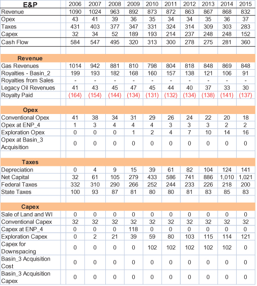
To create “browsing” capability for P&Ls, we need to display summary values always, or on demand. In a conventional P&L, value components and other line items are in rows and time periods in columns. In this case, we collapse the time series in a line-item row by showing its present value (PV) at the left, and collapse the line items in a given time period by showing their net cash flow at the top.

11.3.2 TOTAL VALUE AND VALUE COMPONENTS

For financial decisions, detailed data displays like the P&L can be boiled down to what we call value components by considering only the PVs of the time series (i.e., rows).

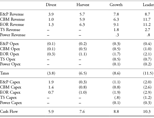
Table 11.2 shows the value components for RNAS. The business units are Exploration and Production (E&P), Enhanced Oil Recovery (EOR), Coalbed Methane (CBM), Tar Sands (TS), and Electric Power. Revenues are positive, and the Opex and Taxes are negative. Capex is usually negative; however, the positive numbers for Capex for the Divest strategy reflect the divestiture proceeds.

TABLE 11.2 RNAS Value Components ($ Billions)

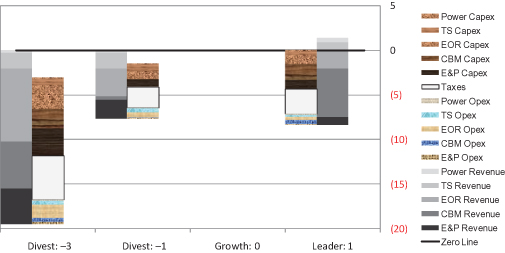
The value components chart presented in Section 9.8.1 allows the value components of multiple strategies to be shown in one chart by displaying all components for a strategy in just two columns, one for negative and one for positive components. Figure 11.6 shows the components of expected value for each strategy in the RNAS example.

FIGURE 11.6 RNAS value components chart.

The first thing to do with the value components chart is to test the composite perspective it portrays:

• Do we believe the value components for each strategy?
• Do we believe the relative value components across strategies?
• Do we believe the value ranking that emerges from the parameters in the value model?

In the value components chart for RNAS, we can see that:

• Strategies with larger revenues require larger investments.
• Taxes are the most significant cost factor.
• The Leader alternative looks best based on total value.
• The Divest alternative looks worst based on total value.

Additional decision insights can be generated by creating a chart showing the difference in value components between strategies. In this way, value components that are common to all strategies cancel out, allowing the ones that differentiate the strategies to stand out. To do this, select a reference strategy, and then for each value component of each strategy, subtract out the corresponding value component of the reference strategy, and then plot in the two-column fashion as before. Typically, it is informative to choose a reference strategy that is fairly good, but not the best. A “status quo” or “momentum” strategy can also be a helpful reference point.

Figure 11.7 displays the RNAS delta value components, where the Growth strategy is used as the reference strategy. For Divest and Harvest, the revenue components are less than the reference (Growth), so in the delta chart, they are negative and show up in the left column.

FIGURE 11.7 RNAS value components, as compared with the Growth strategy.

The point of this graphic is that a relatively small number of blocks have large size, and these are immediately apparent. For RNAS, the most salient blocks are the high CBM revenues for Leader, and the low (absent) CBM revenues and EOR revenues for Divest. This tells us that the decision is mostly about CBM. For Divest, the substantial size difference between the CBM or EOR revenues forgone and the corresponding Capex benefits (= sales proceeds) suggest that sale of those assets is not advantageous.

When possible, it is helpful to use colored graphics for delta value components charts, because the components can shift sides between positive and negative.

As the RNAS experts considered an early version of this chart, they felt that the model yielded too optimistic a portrayal of EOR and CBM. This led them to identify key uncertainties that could reduce value: the probability of outright failure at EOR fields, and the possibility of substantial dewatering delay at CBM. After these issues were addressed, these BUs still looked attractive, and points of weakness in the analysis that had material impact were improved upon.

If there are tradeoffs between one objective or value component and another, here are some ways to use them to develop an improved strategy:

• Enhance a favorable item.
• Minimize or mitigate an unfavorable item.
• Optimize for a different value measure.
• Find a better compromise among the objectives implicated in the tradeoff.

Note that a richer and more varied set of strategies is apt to unearth a broader variety of ways to find value. These will show up as advantages in one Value Component or another, and give additional opportunities to create an improved hybrid strategy (Keeney, 1992).

11.3.3 CASH FLOW OVER TIME

While senior executives normally accept PV discounting, the results of time discounting and the rank-ordering this gives to the strategies may not be immediately obvious or compelling to them. In addition, it abstracts away specific timing of events, which may be of interest. If strategies have distinctly different time profiles of cash flow, it can be helpful to show the cash flow profiles of the strategies together on one chart. This way we can ask the decision team:

• Do you believe the time profile for each strategy?
• Do you believe how the profiles change from one strategy to the next?
• Do you affirm the value ordering implied by your stated time discount rate?

For most of the analyses discussed here, EV of uncertainties is the cleanest approach. For cash flow over time, the EV approach appropriately represents the aggregate impact of benefits when there is a probability of failure, or downstream optionality. However, this must be balanced against the tendency of an EV cash flow to give a misleading view of the duration of investment when the timing of the investment is uncertain—if the investment takes place in a short time period but the time when it starts is uncertain, the EV chart will spread the investment amount over a range of years. A pseudo EV (see Section 9.5.3) chart can be advantageous in such cases, because it distributes investment over a typical time duration starting at a typical time point, rather than spreading it across all possible years.

Figure 11.8 shows the expected cash flow profiles of the four initial RNAS strategies through time. This chart shows that the Leader strategy, which looks very favorable, delivers little positive cash flow during early years. To RNAS management, this was a jarring realization, insofar as North America had been viewed as a source of cash to fund overseas investment.

FIGURE 11.8 RNAS EV cash flows.

Having affirmed this view of the strategies, we can look for ways to improve: Can we accelerate benefits? Can we delay costs? How can we obtain early information on key uncertainties before we commit to major capital and operational expenses?

11.3.4 DIRECT EV TORNADO DIAGRAM

As discussed in Section 9.8.2, an informative way to understand the impact of uncertainty is via sensitivity analysis, which identifies the impact on value of varying each uncertainty in turn from low input to high input. To manage the other dimensions of decision complexity, we choose a strategy, take NPV value across time (or some other metric of interest), and aggregate Business Units.

We display the results of sensitivity analysis in the form of a tornado diagram. In an EV tornado diagram, the value axis is horizontal, and each uncertainty is represented by a horizontal bar from the conditional EV generated by its “low” input to the conditional EV generated by its “high” input. These bars are then sorted with the largest bars at the top, to call attention to variables with the greatest impact on expected value. We call a tornado diagram addressing a chosen strategy a “direct” tornado diagram.

With Monte Carlo simulation, it is not necessary to run a separate simulation to calculate the conditional EV for each end of each tornado bar. Instead, the complete EV tornado diagram can be calculated from the tabulated inputs and outputs of one set of simulation trials. For each uncertain input, the subset of trials in which that input is at its “low” setting is identified, and the expected value of the output value metric is calculated for that subset (by summing the values and dividing by the number of trials in the subset). This expected value is one end of the EV tornado bar for the input parameter. The same procedure is used for the “high” setting of the input to get the other end of the tornado bar. For purposes of this procedure, if an input is sampled from a continuous probability distribution, we define as a “low” input setting anything below the P30 (if the 30/40/30 discretization is used) or P25 (if the 25/50/25 discretization is used). Similarly, a “high” input setting is anything above the P70 or P75.

The direct tornado diagram is a standard feature of most decision analysis software. The user specifies low and high settings for the input parameters and the tornado diagram is calculated and displayed. However, while deterministic tornados are widely available, fewer packages offer EV tornado diagrams.

Figure 11.9 shows the most sensitive variables from the EV tornado diagrams for the four RNAS strategies.

FIGURE 11.9 RNAS direct tornado diagrams, $B.

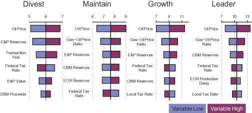
It was not surprising to find the prices of oil and gas at the top of the direct tornado diagram for all the RNAS strategies. Fairly wide ranges of uncertainty about effective taxation rate represented the belief that substantial tax relief might be available.

After developing an EV tornado diagram, review it with the decision team. Compared with the deterministic tornado, whose center line is the base case value or pseudo EV (see Section 9.8.2), the EV tornado helps the decision makers become more familiar with the true probability-weighted average value of the strategy, which is the ultimate decision criterion.

Compare the large bars of the EV tornado to the factors the decision team thinks should be important, and identify anything additional or missing in the tornado. Check the direction of each bar against intuitions about which direction it should point. Each point where intuitions differ from the result of the analysis constitutes a “tornado puzzle.” Tornado puzzles are a great way to develop insights or to identify model errors. If a result does not make sense initially, investigate how it came about and determine whether this makes sense. If it seems wrong, figure out how to improve the model so that it reflects the team’s expertise more closely. If the result holds up, this is an insight for the team. Understand it clearly and explain it to them. As an example, it is interesting to note that in the RNAS Divest Strategy tornado (see Fig. 11.9), the transaction year is a sensitive parameter. This suggests that a later divestment is better than an early divestment. This is consistent with the overall picture that divestment of all assets is less attractive than retaining, developing, and producing the assets; hence, putting off the divestment is attractive.

11.3.5 DELTA EV TORNADO DIAGRAM

An important variant of the tornado diagram is created when we specify two strategies and show the impact of uncertainties on the difference in value between them. The resulting tornado diagram, called the “delta” tornado, highlights the variables that drive the choice between the two strategies. Typically, it is most informative to investigate the delta between two leading strategies. The delta tornado diagram is introduced in Section 9.8.2.

In the RNAS case, having seen the favorable financials for CBM and EOR, the decision team formulated a hybrid strategy with leader-level investment in CBM and EOR, and growth-level investment in E&P. While the ENPV value of this hybrid was very favorable, its investment requirement was high. Accordingly, a similar hybrid was created, identical in all regards except that the legacy E&P assets would be divested instead of being developed. These strategies, which were named Team Hybrid and Divest Hybrid, had very similar ENPVs, indicating that the proceeds from divestment would be as attractive as continued development, as measured by ENPV. Furthermore, as shown in the left and center of Figure 11.10, the direct tornado diagrams for the two strategies were very similar, leaving the team to wonder whether the analysis could shed any light on the choice between them. However, a delta EV tornado (Fig. 11.10, right) showed that the strategies were different and identified what drove the difference. Oil price, tax rates, and variables related to CBM and EOR affected both strategies equally and “canceled out” in the delta tornado, leaving at the top only the variables that drove the difference in value for this decision. The variables affecting the relative value of the Team Hybrid and Divest Hybrid were the gas price that would be realized if the E&P assets were retained and the market value of E&P assets if they were divested.

FIGURE 11.10 Direct and delta tornado diagrams for team hybrid and divest hybrid.

A large bar in a delta tornado diagram that crosses zero indicates that additional information about this variable might cause us to change our decision. Accordingly, it can be worthwhile to convene experts to consider whether there is some way to gather information about any of the leading variables in the delta tornado diagram before the decision must be made. If there is an information-gathering approach, we reformulate the decision model to reflect the option to gather the information, and test whether a strategy embodying this option is worthwhile.

The value of being able to make a decision in light of information to be gained in the future is at the heart of the “real options” approach to valuation (Smith & Nau, 1995). While this was not possible for E&P divestment at Roughneck, Section 11.3.8 shows where this was worthwhile.

11.3.6 ONE-WAY AND TWO-WAY SENSITIVITY ANALYSIS

The delta tornado diagram provides a comparison across many input parameters of how changes in those parameters affect value. It is sometimes insightful to focus on just one input parameter and see how the values of strategies are impacted by changes in that parameter. This is called one-way sensitivity analysis.

Figure 11.11 displays an example of one-way sensitivity analysis. It shows how the values of the two hybrid strategies in the RNAS case vary with changes in the input parameter Gas Price. In this example, the range of uncertainty in the parameter is divided into five equally likely intervals (“quintiles”), and the conditional ENPV is shown for each of the two strategies given that the parameter is in each quintile. We can see that both strategies increase in value as the Gas Price increases but that the value of the Team Hybrid strategy rises faster than does that of the Divest Hybrid strategy, because Team Hybrid has more gas production to sell.

FIGURE 11.11 One-way sensitivity analysis of RNAS hybrid strategies to Gas Price.

The idea behind one-way sensitivity analysis can be extended to show how the values of strategies are affected by changes in two input parameters taken together. This is called two-way sensitivity analysis. A graphical representation of two-way sensitivity analysis would be a three-dimensional chart showing a value surface for each strategy above a two-dimensional space of combinations of settings of the two parameters. A two-dimensional rendition of such a chart would likely be too complicated to produce useful insights. Instead, the results of two-way sensitivity analysis are best shown in tabular form, subtracting one strategy’s value from the other’s.

Table 11.3 shows an example of two-way sensitivity analysis. This table shows the difference in conditional ENPV for the two RNAS hybrid strategies for each of 25 combinations of settings of two input parameters: Gas Price and E&P Value. These variables were chosen to represent the top variables from the delta tornado diagram. Gas Price itself was used, rather than the Gas–Oil Price ratio, to make the chart more easily comprehensible. As in the one-way sensitivity analysis example, the range of uncertainty for each parameter is divided into five quintiles, so the probability that the actual settings of the two parameters will be in any given cell of the table is 4%.

TABLE 11.3 Two-Way Sensitivity Analysis of RNAS Hybrid Strategies to Gas Price and E&P Value

We can see from the table that the value delta between Team Hybrid and Divest Hybrid is greatest when Gas Price is high and E&P Value is low (upper right-hand corner). This indicates that Team Hybrid does better when gas price is high (because it retains more gas production), while Divest Hybrid does better when the price paid for divested assets is high.

The shaded cells in the table indicate the combinations of settings of the two parameters for which the Divest Hybrid has the higher ENPV.

11.3.7 VALUE OF INFORMATION AND VALUE OF CONTROL

Two powerful concepts in decision analysis that should be a part of every value dialogue are the value of information and the value of control.

11.3.7.1 Value of Information. 

An important question to ask is the following: How much more valuable would this situation be if we could resolve one or more of the key uncertainties before making this decision? The answer to this question is the value of information. We make a distinction between perfect and imperfect information. We often call perfect information clairvoyance, because it is what we would learn from a clairvoyant—a person who perfectly and truthfully reports on any observable event that is not affected by our actions (R. Howard, 1966). Whereas clairvoyance about an uncertain parameter eliminates uncertainty on that parameter completely, imperfect information reduces but does not eliminate the uncertainty. Despite the fact that almost all real-world information about the future is imperfect, we tend to calculate the value of clairvoyance first because it is easier to calculate than the value of imperfect information and it sets an upper limit on the value of imperfect information in the current decision context. If the value of clairvoyance is low or zero, we know that we need not consider getting any kind of information on that parameter for the decision under consideration. Of course, information that has zero value for one decision might have positive value for another. For instance, information on oil price periodicity may have no value for making long-term strategic decisions for a petroleum company, but it could have high value for a decision about whether to delay the construction of a petrochemical plant.

Calculating the value of clairvoyance is fairly straightforward. It involves restructuring the probabilistic analysis so that the choice of strategy is made optimally after the uncertainty in question is resolved. If the analysis is structured as a decision tree, this is equivalent to moving the uncertain node in front of the decision node. This may require using Bayes’ rule to redefine conditional probabilities if this uncertainty is dependent on another. In most cases,³ the value of clairvoyance is the difference between the optimal value in this restructured tree and the optimal value in the original tree.

Figure 11.12 shows the calculation of value of clairvoyance on whether or not royalty payments are required in the capacity planning example presented in Section 11.2.1.1. The figure shows only the start of the restructured decision tree, with the royalty uncertainty now coming before the decision on initial capacity. We see that if we know in advance that royalties will be required, we would choose Low initial capacity; but if we know that royalties will not be required, we would stick with the original optimal choice of Flexible initial capacity. The expected NPV of this new situation is $65 million, compared with $64 million for the situation without clairvoyance. So the value of this clairvoyance is the difference, $1 million.

FIGURE 11.12 Calculating value of clairvoyance on royalty in capacity planning example.

It can be helpful to systematically calculate the value of clairvoyance on each uncertain parameter. Typically, the value is zero for many parameters. It may also be worthwhile to calculate the value of clairvoyance on combinations of two or three parameters together, particularly if such combinations correspond to actual information-gathering possibilities. The value of information cannot be negative. And the value of information on a combination of uncertain parameters together is not always equal to the sum of the values of information on those parameters taken individually.

Some influence diagram/decision tree software will automatically calculate the value of information on each uncertain variable in the decision tree.

Virtually all information-gathering opportunities considered in professional practice involve information that is imperfect rather than perfect. Calculating the value of imperfect information uses the same logic as calculating the value of clairvoyance—determine how much the overall value of the situation increases because of the information. The actual calculation is somewhat more involved, generally requiring the use of Bayes’ rule to calculate conditional probabilities in a restructured tree. Section 11.3.8 illustrates how the price of oil current at the time of a decision can be used as valuable imperfect information on long-term oil prices.

Delta EV tornado diagrams give us some indication of which parameters have positive value of clairvoyance. On a delta EV tornado diagram comparing the optimal strategy with another strategy, any parameter whose bar crosses the zero delta value line has positive value of clairvoyance.

In the value dialogue, we can use the calculated value of clairvoyance to improve the decision in several different ways. The first is obvious—create a new strategy that includes initial information gathering on a parameter with high value of clairvoyance before the main decision is made. This might be a diagnostic test, a market survey, an experimental study, or a pilot plant. When evaluating such a strategy, it is important to characterize the degree to which the actual information gathered will be imperfect—how will the probabilities of the possible outcomes of the parameter in question change with the gathered information? Also, it is important to include the cost, if any, of delaying the decision in such a strategy.

Another possibility is to design a new strategy that builds-in flexibility, effectively deferring the decision until after the uncertainty is resolved. For example, in a production planning decision, if sales demand has high value of clairvoyance, it might make sense to use a temporary means of production (e.g., outsourcing) for a few years and then commit to investing in internal capacity with better knowledge of demand. (See also the discussion of real options in Section 11.3.8.) Also, it might be possible to incur a cost to speed up the resolution of an uncertainty with high value of clairvoyance.

11.3.7.2 Value of Control. 

The value of control is a concept analogous to that of the value of information. Here, we ask the question: How much more valuable would this situation be if we could make a key uncertainty resolve in our favor? The mythical character in this case is the Wizard—the one who can make anything happen at our request.

It is a simple matter to calculate the value of perfect control (assuming that the decision maker either is risk neutral or adheres to the delta property—see Section 11.4.1). Fix the parameter in question to its most favorable setting and run the probabilistic analysis for all strategies, observing the highest EV among them. The difference between that EV and the EV of the best strategy without control is the value of control. The value of perfect control can be found quite easily from direct EV tornado diagrams—simply subtract the original EV from the highest value among the right-hand ends of the parameter’s tornado bars for all strategies. Similarly, if the value of clairvoyance on a parameter has been calculated by restructuring a decision tree, the value of perfect control can be found by observing the EV of the most preferred branch of the parameter in the restructured tree. For example, in the restructured tree used to calculate the value of clairvoyance on whether or not royalty payments are required in the capacity planning example (see Fig. 11.12), we see that if royalties are not required, the EV is $81 million, so the value of perfect control on the royalty issue is $17 million ($81–$64 million).

We can use the calculated value of control to guide our thinking about how to create a better strategy. For each parameter with high value of control, we ask: What could we do to make the favorable outcome more likely to occur? Sometimes, the range of uncertainty that we have assessed for a parameter is based on an assumed constraint that, in reality, can be eased at some cost. For example, the range of uncertainty on how long it will take to get a new pharmaceutical product to market might be based on an assumed fixed budget for clinical trials. If the value of control on time to market is high (as it often is in that industry), then it might be that the range on time to market can be shifted in our favor by increasing the clinical trials budget. A better strategy can be created in this case if the increase in expected value due to earlier entry exceeds the cost of additional budget.

In the capacity planning example, the realization that the value of the situation increases by $16 million if we can ensure that royalties are not required may stimulate the creation of a new alternative—offering to settle the patent infringement lawsuit out-of-court for a payment of less than $16 million.

11.3.8 REAL OPTIONS

For Roughneck, Tar Sands⁴ was a new technology. There was a large risk that the economics might not pan out, so Roughneck wanted to take a cautious incremental approach, beginning with construction and operation of a pilot plant, which takes many years. Subsequent large investment in full-scale development would be made only if a favorable trigger event were seen. The decision team proposed many triggering factors: new technology, regulatory support, improved oil pipeline infrastructure, or successes of competitors in analogous efforts. However, preliminary analysis did not find much value in any of these triggering strategies.

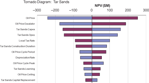
If Roughneck were required to precommit to full-scale Tar Sands development, the program’s value increment would not be favorable enough to be funded, so there would be no reason for preliminary technology development or construction of a pilot plant. Even so, we analyzed this simple precommitment strategy to identify its value drivers and used these insights to develop a more valuable plan. We found that consideration of the business-unit-specific tornado for this strategy (Fig. 11.13) allowed us to create a contingent approach that increased the value of the program substantially. High oil price can make the value increment substantially positive. By the time the pilot plant is finished, Roughneck will have additional information about the long-term level of oil price. This suggested a contingent (or real option) strategy that would build the pilot plant, but only move to full-scale development if the then-current oil price exceeds a threshold.

FIGURE 11.13 Tar sands tornado diagram.

At the time of the analysis of precommitment to full-scale development, the model of oil price was simple: a range of possible oil prices at a fixed time point, and a range for the oil price escalator in subsequent years. We realized that testing contingent strategies against this orderly and predictable model of prices would overstate the value of the information seen at the decision point for full development, and thus overstate the value of the contingent strategy. So we worked with the oil price experts to more appropriately reflect the factors that inform the company’s view of future long-term oil prices: cyclicality (with partially understood period, amplitude, and phase), and volatility. Roughneck experts judged that a simulation that handled these issues properly would have enough noise that the information conferred by observing the value at the time the decision has to be made (10 years in the future) would be informative, but without overstating the value of that information. Hence, we added parameters for these uncertainties, assessed their plausible ranges, and added them to the simulation.

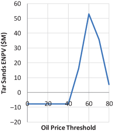
We then simulated strategies that would build the full-scale Tar Sands facility only if the then-current oil price exceeded a threshold. We added a decision column to the strategy table to represent the threshold oil price at which Tar Sands would go forward, and added logic to the model to implement this decision rule. We then created strategies that differed only in the Tar Sands threshold, in order to test thresholds of $40, $50, $60, $70, and $80 dollars per barrel. We simulated these strategies and noted the Tar Sands ENPV value of each option. A threshold of $60/bbl seemed best, improving the program from break-even to ENPV of roughly $50M. See Figure 11.14. As we discuss in the next section, this level of threshold reduces the likelihood of unfavorable investment while still allowing favorable investment to be made.

FIGURE 11.14 Tar sands construction threshold exploits optionality.

11.3.9 S-CURVES (CUMULATIVE PROBABILITY DISTRIBUTIONS)

When a favorable strategy has a big downside, we can use the S-curve of the value measure to understand how much risk we are facing, and how well a proposed response may reduce that risk.

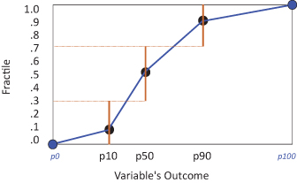
An “S-curve” (or cumulative probability distribution) depicts the probability that value achieved (or any other objective) is at or below any given level, that is, its fractile. In the conventional layout for S-curves, value is on the x-axis, and the cumulative probability is on the y-axis. Hence, in an S-curve, the “upside” is to the right, not up. To chart an S-curve, sort in order from lowest to highest the instantiated values from Monte Carlo simulation and juxtapose these with the position number, going from 1 to N, the total number of values. Then calculate the cumulative probability for each value in the list by dividing its position number by N. An S-curve is a line plot of these value-cumulative probability pairs. S-curves are automatically generated by decision tree and Monte Carlo software.

S-curves are a very useful analytical tool. However, it is important to understand that decision makers and stakeholders may have difficulty understanding the S-curve. In organizations without a culture of using probabilistic decision analysis, it will be important to clearly explain the S-curve. Some decision makers are more comfortable looking at the flying bar charts (next section) or probability density functions, which can show similar information.

Once we see the downside risk of our best alternatives, we look for ways to modify the strategies to mitigate the risk.

If the S-curve for the leading strategy is wholly to the right of the others, it is said to be “stochastically dominant.”⁵ This means that it is more likely to deliver any specified level of value than any other strategy. It also means that the strategy is preferred over the others regardless of risk attitude.

If two S-curves cross over and there is a large downside on the NPV distribution of one, and if the decision maker feels this downside constitutes a substantial risk, this would call into question using ENPV as the decision criterion. In this case, we would need to take risk attitude into account explicitly by assessing a true utility function (see Section 11.4), rather than using ENPV as a surrogate utility function.

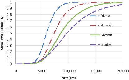
Figure 11.15 shows the S-curves for NPV value for the four RNAS strategies. We found that the strategies’ S-curves did not cross significantly, which meant that there was no risk–value tradeoff to be made. More ambitious strategies generated more upside, but their downsides were not worse. Some decision team members found this counterintuitive, because larger strategies require higher investment. However, for RNAS, the investment was incremental through time, with plenty of feedback, so there was never much investment truly at risk. None of the downsides was viewed as serious enough to call for a utility function to be formulated; so maximizing ENPV was used as the decision criterion.

FIGURE 11.15 RNAS S-curves.

As always, we start by asking the decision team the following questions:

• Do you believe the value profile for each strategy?
• Do you believe how the value profiles change from one strategy to the next?
• Do you affirm the ordering implied by your stated risk attitude (if pertinent)?

Having done so, we ask whether we can enhance the upside or mitigate the downside (reduce the risk) of a leading strategy. On its own, an S-curve gives little guidance where to look for such an enhancement. We should look instead at the tornado diagram (or the “Contribution to Variance” output provided by some Monte Carlo software packages) to identify the biggest drivers of uncertainty in value, which typically are the ones that drive the downside risk.

An S-curve is more useful as a description of a strategy’s potential outcomes than as a spur to creativity. For example, we used business-unit S-curves to understand how an oil price threshold added value to Roughneck Tar Sands strategies.

The S-curves in Figure 11.16 show the value profiles of Tar Sands development, using various thresholds. The wedge between the vertical axis and an S-curve on the right measured the upside, while the wedge between the axis and the curves on the left measured the downside. From $40 to $50 to $60, reductions of downside (from eliminating unfavorable investment) were large, with little reduction to upsides (investment that would have been favorable), and so expected value improved. But past $60 to $70 and $80, there was not so much downside to mitigate, and the reductions of upside predominated, and so expected value decreased.

FIGURE 11.16 Tar sands value-risk profiles.

For a complex decision situation like RNAS Tar Sands, there were too many uncertainties and decision opportunities to be displayed intelligibly as a full decision tree, and representing them all at requisite granularity in the analysis software would require a huge multidimensional data structure. However, once we had made the decision and wanted to show its logic to senior stakeholders, a simplified decision tree was useful. This is discussed in the Chapter 13.

11.3.10 FLYING BAR CHARTS

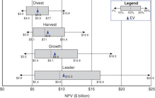
A chart showing S-curves for several different strategies might not be the best way to convey insights to decision makers, particularly if the S-curves cross each other, because the insights are obscured by the detailed information in the chart. Instead, a simpler chart, called a “flying bars” chart,⁶ might be a more effective way to display meaningfully a comparison of the uncertainty and risk in the strategies. The flying bars chart shows only a small subset of the information in an S-curve: a few percentiles plus the EV. Figure 11.17 shows the flying bars chart for the four original RNAS strategies that are displayed as S-curves in Figure 11.15. The ends of each bar in the chart are the P10 and P90 NPVs for the strategy, while the ends of the arrows are the P1 and P99 NPVs. The P50 NPV is shown as a dashed line, and the EV is indicated by a triangular shape. For an even simpler chart, the P1 and P99 arrows and the P50 line may be omitted.

FIGURE 11.17 Flying bars chart for RNAS strategies.

11.4 Risk Attitude

Many decisions can be made using the criterion of maximizing EV. However, if the S-curves for the strategies reveal significant downside risk and if none of the strategies stochastically dominates the others (i.e., has an S-curve that is completely to the right all other S-curves), then the risk attitude of the decision maker must be taken into account explicitly to find the optimal strategy. To do this, we go back to the Five Rules stated in Chapter 3.

The Five Rules together imply the existence of a utility metric. To be consistent with the Five Rules, decisions should be made to maximize the expected value of that utility metric. But the Five Rules do not specify the form of the utility function that maps value outcomes to the utility metric. The characteristics of the utility function depend on the preferences of the decision maker regarding risk-taking, which we call risk attitude. A person who always values an uncertain deal at its expected value is said to be risk neutral. A person who values an uncertain deal at more than its expected value is said to be risk seeking. This person would willingly pay money to increase the level of risk. In professional practice, we almost never encounter a decision maker who is truly risk seeking. A person who values an uncertain deal at less than its expected value is said to be risk averse. This person is willing to give up some value to avoid risk. The degree of a person’s risk aversion can be measured quantitatively.

11.4.1 DELTA PROPERTY

An appealing addition to the Five Rules is called the delta property, which states that if a constant amount of money is added to every outcome of an uncertain deal, the value of the deal increases by that amount. As an example, let us suppose that someone values at $4000 an uncertain deal that offers equal chances of winning $10,000 and winning nothing. How would that person value the uncertain deal if we add $100 to each outcome (i.e., the modified deal offers equal chances of winning $10,100 and $100)? If the delta property applies, the person would value the modified deal at $4100. This seems to make a lot of sense, since the modified deal is equivalent to the original deal (worth $4000) plus a sure $100. Clearly, it is hard to argue against the delta property as long as the delta amount does not significantly change the person’s wealth.

For someone who wants to make decisions consistent with the Five Rules plus the delta property, the utility function must have one of two forms—either linear or exponential (Howard, 1983).

A linear utility function is appropriate for a decision maker who is risk neutral. This person values every uncertain deal at its expected value, regardless of the level of risk. In other words, a risk neutral decision maker is not willing to give up any expected value to avoid risk.

11.4.2 EXPONENTIAL UTILITY

An exponential utility function is appropriate for a person who is risk averse and who wants to be consistent with the Five Rules plus the delta property. The functional form of the exponential utility function is:

(11.1) 

for B > 0 and R > 0.

The essential properties of any utility function are preserved in a linear transformation (i.e., when constants are multiplied and/or added to the function) (R. Howard, 1983). So the parameters A and B in Equation 11.1 are arbitrary. There is only one parameter (R) that matters for an exponential utility function. This parameter is called risk tolerance, and it is expressed in the same units as the value metric, which is usually in monetary units. (The reciprocal of risk tolerance is given the name risk aversion coefficient in the literature.) The larger the risk tolerance, the smaller the degree of risk aversion. An infinitely large risk tolerance indicates risk neutrality.

11.4.3 ASSESSING RISK TOLERANCE

The approximate value of risk tolerance for any decision maker can be assessed via the answer to just one question (see Fig. 11.18): For what amount of value (e.g., money) Q is the decision maker indifferent between having and not having an uncertain deal offering equal chances of winning Q and losing one-half of Q (McNamee & Celona, 2001)? For small values of Q, the downside risk is small so the positive expected value of the uncertain deal (Q/4) makes it look attractive. But for large values of Q, the 50% chance of losing Q/2 makes the deal look too risky to be attractive.

FIGURE 11.18 Assessing risk tolerance.

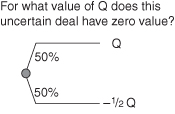
The value of Q that puts this deal on the boundary between attractive and unattractive is a good estimate of the decision maker’s risk tolerance. (The actual risk tolerance is about 4% bigger than Q.)

11.4.4 CALCULATING CERTAIN EQUIVALENTS

Once the value of a decision maker’s risk tolerance has been assessed, it can be used to calculate his or her certain equivalent (CE) for any uncertain deal. The utility metric is calculated for each possible outcome using the utility function. For computational simplicity, the best choice of the two arbitrary parameters for the exponential utility function in Equation 11.1 are A = 0 and B = 1, yielding the utility function:

(11.2) 

The probability-weighted average of the utility metric (i.e., the expected utility) is calculated for the uncertain deal and the certain equivalent is found via the inverse of the utility function:

(11.3) 

where U is the expected utility.

11.4.5 EVALUATING “SMALL” RISKS

Knowing the appropriate value of risk tolerance, we can easily calculate the certain equivalent for any uncertain deal for which the delta property applies.

Consider the chart in Figure 11.19, which shows the calculated certain equivalent and the expected value for uncertain deals of different “sizes.” The deal is a 75% chance of winning an amount Q and a 25% chance of losing that amount Q. The chart shows the EV and CE for different amounts Q expressed as a percentage of the risk tolerance. Note that for deals that are quite “small” relative to the risk tolerance (<10%), the expected value and the certain equivalent are very close. This suggests that for “small” risks, we do not need to calculate the certain equivalent but instead can use the expected value as a very good approximation of it.

FIGURE 11.19 EV and CE versus size of deal.

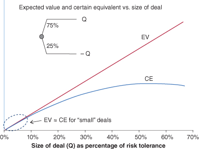
But how do we know if an uncertain deal is “small” enough to use EV rather than CE as the decision criterion? If we have assessed the risk tolerance, we can apply a simple rule of thumb—If the range of outcomes (from best to worst) in a deal does not exceed 5% of the risk tolerance, use the EV; otherwise, calculate the CE. If we have not yet assessed the risk tolerance, we can sometimes make a very rough guess as to what it would be if we were to assess it. One study (McNamee & Celona, 2001) suggests that a company’s risk tolerance is roughly equal to 20% of its market capitalization. If we use this rough estimate along with the rule of thumb stated above, we should feel comfortable using EV as the decision criterion for uncertain deals whose range of outcomes is less than 1% of the company’s market capitalization. However, if in doubt, always check with the decision maker.

11.4.6 GOING BEYOND THE DELTA PROPERTY

Very occasionally, we may encounter a decision situation with a range of possible outcomes so big that the delta property no longer applies. This would be a situation in which at least one of the possible outcomes would significantly change the wealth of the decision maker and thus change his or her attitude toward risk-taking. In such a situation, the utility function would have a different form than the exponential and assessing it would require more than one question.

We believe that the risk preferences of most decision makers would be characterized by decreasing risk aversion as wealth increases. As an illustration, consider an uncertain deal offering equal chances of winning $200,000 and winning nothing. A person with relatively little wealth might prefer to receive a certain $50,000 instead of the uncertain deal because of its substantial risk of paying out nothing. But if that same person suddenly became a multimillionaire, he or she might then prefer the uncertain deal to the certain $50,000 because the expected value of the deal is twice as great.

A particularly interesting form of decreasing risk aversion is called the one-switch rule (Bell, 1988). This rule states that for every pair of alternatives whose ranking depends on wealth, there exists a wealth level such that one of the alternatives is preferred below that level and the other is preferred above it. The rule seems to be quite easy to accept. Consider two uncertain deals: Deal A offers equal chances of winning $100,000 and winning $50,000 (EV = $75,000). Deal B offers equal chances of winning $200,000 and winning nothing (EV = $100,000). We would not be surprised if a decision maker prefers Deal A at low levels of wealth but then switches to preferring Deal B at a higher level of wealth. But we would find it quite surprising if that same decision maker switches back to preferring Deal A at an even higher level of wealth.

The form of utility function that is consistent with the one switch rule is the linear plus exponential:

(11.4) 

for A ≥ 0, B > 0 and C > 0.

11.5 Illustrative Examples

See Table 1.3 for further information on the illustrative examples. The probabilistic analysis of our RNAS is described in Section 11.3. The next sections describe probabilistic analysis for the Geneptin and data center examples.

11.5.1 GENEPTIN EXAMPLE

The Geneptin team conducted probabilistic analysis using an Excel model with Crystal Ball^©. The simulation gave probabilities of 25/50/25 to the P10, P50, and P90 inputs assessed by the experts. The resulting P10-P50-P90 range of NPV and mean (EV) for the two strategic alternatives are shown in the flying bar chart in Figure 11.20.

FIGURE 11.20 Geneptin flying bar chart.

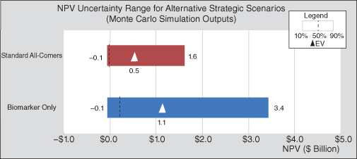
To communicate with stakeholders from multiple functional areas, the DA team members used tools like the waterfall chart in Figure 11.21 to illustrate how much each value driver impacts the value Geneptin generates.

FIGURE 11.21 Geneptin waterfall chart.

11.5.2 DATA CENTER

In the real data center problem, probabilistic analysis was not performed because of tightness in the decision schedule and because some of the key uncertainties were reduced by actions taken by the implementation team.

In a different setting, a decision tree or a Monte Carlo analysis could have been performed on the data center problem. When doing probabilistic analysis for a MODA model, we need to consider if the uncertainties are dependent or independent. If the major uncertainties are the scores and these are independent, we typically use Monte Carlo simulation. If there are major interdependent uncertainties that impact several scores, a decision tree may be a more effective tool (Parnell et al., 2011).

11.6 Summary

There are two important ways to add value: choose correctly among identified strategies and improve upon the selected strategy by increasing the value and/or reducing the risk of the downside consequences. Once we have developed a preliminary version of a composite perspective on what drives value, we undertake a value dialogue with the decision team aimed at verifying the authenticity of the composite perspective, and use it to choose correctly and find even more valuable and less risky strategies.

Of the five dimensions of complexity in a decision situation (value components, alternatives, uncertainty, business units, and time), the most difficult to manage is uncertainty, since it requires more information to analyze and is more difficult to explain to the decision team. There are two main methods to analyze uncertainty: decision trees and simulation. A decision tree sets all but a small number of parameters to fixed values, discretizes the rest, and considers all possible combinations, developing an approximate EV and set of contingent decisions for the problem as structured. The simulation method samples randomly from inputs for all uncertain parameters, giving EV results that can be made arbitrarily close to the true EV answer if a sufficient number of samples is chosen. It gives guidance on construction of contingent decision rules; however, these are more difficult to obtain than with decision trees.

Either way, a large number of scenarios are considered, alongside complexity from the other four dimensions. To manage this complexity and facilitate the value dialogue, we take various two- or three-dimensional slices of value outcomes, while collapsing the other dimensions. While there are various ways to collapse dimensions, the typical approaches are:

• Look at value and value components of each strategy, or look at the delta between two strategies.
• Take EV across uncertainty outcomes.
• Aggregate across business units or opportunities.
• Calculate the PV cash flow across time.
• Aggregate value measures/objectives to utility.

There is a set of analyses that are frequently useful. For each analysis, the value dialogue has two phases:

• Compare the composite perspective with individual perspectives of the decision team, aiming to improve one or the other where they differ.
• Use the improved perspectives to search for ideas that could further improve the actions we can take.

Here are some important analyses and their purposes:

• Value components chart, to show how much of each value component is created by each strategy, and spur thought on how to combine different strategies’ successful approaches
• Cash flow profiles of strategies, to highlight any time tradeoffs and spur thought on timing of costs or benefits.
• Direct tornado for a leading strategy, to identify opportunities for improvement by controlling a key uncertainty.
• Delta tornado of the best strategy versus another leading strategy, to ascertain whether the outcome of any uncertainty could change the decision, to guide information gathering or construction of a contingent strategy.
• S-curves (cumulative probability curves) for strategies’ NPVs, to show whether there is any risk-value tradeoff.

If a promising new strategy is developed, we sometimes need to elicit additional expertise to ascertain its consequences properly, but typically this effort is small compared to the overall analysis effort.

KEY TERMS

Notes

¹If the expert has assessed only P10, P50 and P90, we choose P0 ≡ 2.5*P10 − 1.5*P50 and P100 ≡ 2.5*P90 − 1.5*P50. These formulas for P0 and P100 were chosen so that the resulting fractile curve resembles Gaussian, lognormal and other common distributions. The derivation of the P0 and P100, and their use to generate a distribution that is similar to other well-known distributions is due to Rob Brown. Brown generated a smooth fractile curve by fitting an increasing spline to the five fractiles. Brown–Johnson substitutes piecewise linear.

²On a computer, the Monte Carlo samples are actually generated via well-designed pseudo-random number algorithms whose initial “seed” is usually taken from a hard-to-predict source, such as the system clock.

³The simple calculation of the value of clairvoyance is valid if the decision maker is risk neutral or is risk averse and accepts the delta property (see Section 11.4.1).

⁴Tar sands (also called oil sands) is a combination of clay, sand, water, and bitumen, a heavy black viscous oil. Tar sands are mined and then the oil-rich bitumen is extracted.

⁵Early works also refer to the notion of “deterministic dominance,” which is seen when the 0th percentile of one strategy exceeds the 100th percentile of another. Situation exhibiting such extreme superiority rarely arise, so the term is not often useful in practice.

⁶These charts are commonly called box and whisker charts or stock charts in Excel.

REFERENCES

Asmussen, S. & Glynn, P. (2007). Stochastic Simulation: Algorithms and Analysis. New York: Springer.

Bell, D. (1988). One-switch utility functions and a measure of risk. Management Science, 34(12), 1416–1424.

Bueno De Mesquita, B. (2002). Predicting Politics. Columbus: Ohio State University Press.

Forrester, J. (1961). Industrial Dynamics. Waltham, MA: Pegasus Communications.

Howard, R. (1966). Information value theory. IEE Transactions on Systems Science and Cybernetics, 2(1), 22–26.

Howard, R. (1983). The evolution of decision analysis. In R. Howard & J. Matheson (eds.), The Principles and Applications of Decision Analysis, pp. 5–16. Menlo Park, CA: Strategic Decisions Group.

Keefer, D. (1994). Certainty equivalents for three-point discrete-distribution approximations. Management Science, 40(6), 760–773.

Keeney, R. (1992). Value-Focused Thinking. Cambridge, MA: Harvard University Press.

Lindley, D. (1987). Using expert advice on a skew judgmental distribution. Operations Research, 35(5), 716–721.

Luce, D. & Raiffa, H. (1957). Games and Decisions. New York: John Wiley & Sons.

McNamee, P. & Celona, J. (2001). Decision Analysis for the Professional. Menlo Park, CA: SmartOrg, Inc.

Papayoanou, P. (2010). Game Theory for Business. Sugar Land, TX: Probabilistic Publishing.

Parnell, G.S., Driscoll, P.J., & Henderson, S. (eds.). (2011). Decision-Making, 2nd ed. New York: John Wiley & Sons.

Raiffa, H. (1968). Decision Analysis: Introductory Lectures on Choices Under Uncertainty. Reading, MA: Addison-Welsey Publishing Co.

Robinson, S. (2004). Simulation: The Practice of Model Development and Use. Chichester: John Wiley & Sons.

Smith, J. & Nau, B. (1995). Valuing risky projects: Option pricing theory and decision analysis. Management Science, 41(5), 795–816.