CHAPTER 11
Process Benchmarking With Data Envelopment Analysis
Data envelopment analysis (DEA), introduced by Charnes, Cooper, and Rhodes (1978), is a linear programming method for calculating relative efficiencies of a set of organizations that possess some common functional elements but whose efficiency may vary due to internal differences. One main difference, for instance, might be the management style employed in each organization. In DEA, organizations are referred to as decision-making units (DMUs).
DEA has generated a fair amount of interest in the academic world and among practitioners because it has been applied successfully to assess the efficiency of various organizations in the public and private sectors. The popularity of the technique is evident by the increasing number of articles in scientific journals and the popular press. A search of DEA on the Internet results in hundreds of pages that make reference to this methodology1. Recently, DEA has been used as a tool for benchmarking. This chapter discusses the application of DEA to business process benchmarking. When data envelopment analysis is used for benchmarking processes, the process becomes the decision-making unit. Therefore, the terms DMU and process are used interchangeably throughout this chapter.
DEA considers a process as a black box and analyzes inputs and outputs to determine relative efficiencies. The black-box model (or transformation model) is depicted in Figure 11.1 (see also Section 1.1.2 and Figure 1.1), where possible inputs to and outputs from a process are as follows.
Inputs
- Full-time equivalent (FTE) employees
- Office space
- Regular hours
- Overtime hours
- Operating expenses
- Number of computers
- Number of telephone lines

Outputs
- Cycle time
- Cycle time efficiency
- Throughput rate
- Capacity utilization
- Customer rating
- On-time deliveries
Using the black-box approach, the efficiency of a process can be calculated with a simple ratio when there is a single input and a single output.

However, when a process uses multiple inputs and produces multiple outputs, it becomes more difficult to evaluate its efficiency.
Example 11.1
Suppose labor cost and throughput rate are considered a single input and output of a business process, respectively. The efficiency of two processes, say A and B, can be obtained easily as shown in Table 11.1.
Clearly, process A is more efficient than process B, because A is able to complete 0.75 jobs for every dollar spent in labor, but B can complete only 0.733 jobs per dollar. However, the manager of process B might not agree with this assessment, because that manager might argue that efficiency is more directly affected by office space than it is by direct labor costs. The efficiency assessment in this case might be as shown in Table 11.2.
The new assessment shows that process B is more efficient than process A when office space is considered the single input to this process. More realistically, both inputs should be used to compare the efficiency of processes A and B.
TABLE 11.1 Efficiency Calculation Based on Direct Labor Costs

TABLE 11.2 Efficiency Calculation Based on Office Space

The DEA approach offers a variety of models in which multiple inputs and outputs can be used to compare the efficiency of two or more processes. This chapter is limited in scope to the ratio model, which is based on the following definition of efficiency.

Suppose this definition is used to compare the efficiency of the processes in Example 11.1 by considering that the labor cost is twice as important as the cost of office space. In this case, the efficiency of each process can be calculated as follows.

The chosen weights make process B more efficient than process A, but the manager of process A could certainly argue that a different set of weights might change the outcome of the analysis. The manager’s argument is valid, because the weights were chosen arbitrarily. Even if the weights were chosen prudently, it would be almost impossible to build consensus about these values among all process owners. This is why DEA models are based on the premise that each process should be able to pick its own “best” set of weights. However, the weight values must satisfy the following conditions.
- All weights in the chosen set should be strictly greater than 0.
- The set of weights cannot make any process more than 100 percent efficient.
Suppose the owner of process A in Example 11.1 chooses a weight of 0.25 for labor cost and 0.1 for office area. This set of weights makes process A 100 percent efficient.
However, the set of weights is not “legal” when used to compare the efficiency of process A with the efficiency of process B, because the weights result in an efficiency value for process B that is more than 100 percent.
As seen in this example, the weight values can be “legal” or “illegal,” depending on the processes that are being compared. Also, the efficiency of one process depends on the performance of the other processes that are included in the set. In other words, DEA is a tool for evaluating the relative efficiency of decision-making units; therefore, no conclusions can be drawn regarding the absolute efficiency of a process when applying this technique.
Typical statistical methods are characterized as central tendency approaches because they evaluate processes relative to the performance of an average process. In contrast, DEA is an extreme point method that compares each process with only the “best” processes.
A fundamental assumption in an extreme point method is that if a given process A is capable of producing Out(A) units of output with In(A) units of input, then other processes also should be able to do the same if they were to operate efficiently. Similarly, if process B is capable of producing Out(B) units of output with In(B) units of input, then other processes also should be capable of the same production efficiency. DEA is based on the premise that processes A, B, and others can be combined to form a composite process with composite inputs and composite outputs. Because this composite process does not necessarily exist, it typically is called a virtual process.
The heart of the analysis lies in finding the best virtual process for each real process. If the virtual process is better than the real process by either making more output with the same input or making the same output with less input, then the real process is declared inefficient. The procedure of finding the best virtual process is based on formulating a linear program. Hence, analyzing the efficiency of n processes consists of solving a set of n linear programming problems.
11.1 Graphical Analysis of the Ratio Model
Before describing the linear programming formulation of the ratio model, the ratio model will be examined for the case of a single input and two outputs. This special case can be studied and solved on a two-dimensional graph.
Example 11.2
Suppose one would like to compare the relative efficiency of six processes (labeled A to F) according to their use of a single input (labor hours) and two outputs (throughput rate and customer service rating). The relevant data values are shown in Table 11.3. (For the sake of this illustration, do not consider the relative magnitudes and/or the units of the data values.)
The ratio model can be used to find out which processes are relatively inefficient and also how the inefficient processes could become efficient. In order to answer these questions, first calculate two different ratios: (1) the ratio of throughput with respect to labor and (2) the ratio of customer rating with respect to labor. Table 11.4 shows the values of the independent efficiency ratios, where the first ratio is labeled x and the second ratio is labeled y.
TABLE 11.3 Input and Output Data for Example 11.2

TABLE 11.4 Independent Efficiency Calculations

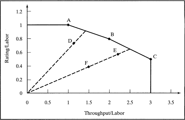
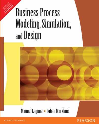
FIGURE 11.2 Efficient Frontier for Example 9.2
The x and y values are used in Table 11.4 to plot the relative position of each process in a two-dimensional coordinate system. The resulting graph is shown in Figure 11.2.
Figure 11.2 shows the efficient frontier of this benchmarking problem. Processes that lie on the efficient frontier are nondominated, but not all nondominated processes are efficient. A non-dominated process is such that no other process can be at least as efficient in all the different performance measures and strictly more efficient in at least one performance measure. The nondominated processes that are in the outer envelope of the graph define the efficient frontier. Under this definition, processes A, B, and C characterize the efficient frontier in Figure 11.2. These also are called the relatively efficient processes. Note that A is better than B and C in terms of the y-ratio, but it is inferior to both of those processes in terms of the x-ratio. Also note that E is a nondominated process that is not efficient, because it does not lie on the efficient frontier.
This graphical analysis has helped answer the question about the relative efficiency of the processes. A, B, and C are relatively efficient processes, and D, E, and F are relatively inefficient. The term relatively efficient or inefficient is used because the efficiency depends on the processes that are used to perform the analysis. In order to clarify this issue, suppose a process G is added with x = 2.5 and y = 1. This addition makes process B relatively inefficient, because the revised envelope moves farther up (i.e., in the direction of the positive y values) relative to the original processes. In the absence of such a process, B is relatively efficient.
11.1.1 EFFICIENCY CALCULATION
Relatively efficient processes (i.e., those on the efficient frontier) are considered to have 100 percent efficiency under the ratio model. What is the relative efficiency value of a process that is relatively inefficient? To answer this question, analyze the situation depicted in Figure 11.3.
This figure shows a relatively inefficient process PO with coordinates (x0, y0) and relatively efficient processes P1 and P2 with coordinates (x1, y1) and (x2, y2), where 
 Because processes P1 and P2 are relatively efficient, input their efficiency value is 100 percent. Also, because the line going from the origin to process P0 intersects the line from process P1 to process P2, these two processes are known as the peer group (or reference set) of process P0.
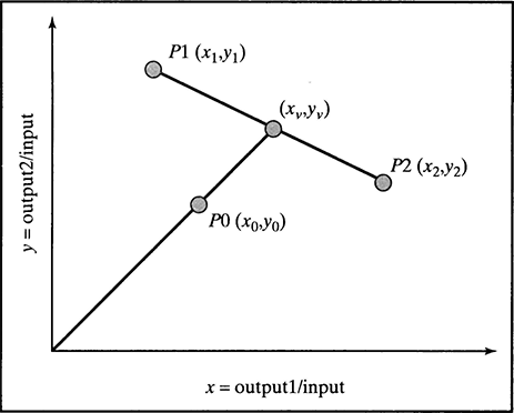
FIGURE 11.3 Projection of a Relatively Inefficient Process
The efficiency associated with process P0 is less than 100 percent, because this process is not on the efficient frontier. The efficiency of process P0 is the distance from the origin to the (x0, y0) point divided by the distance between the origin and the virtual process with coordinates (xv, yv). To calculate the efficiency of process P0, it is necessary to first calculate the coordinates of the virtual (and efficient) process. This can be done using the following equations.

Then the efficiency of process P0 is given by:

To illustrate the use of these equations, consider process D in Tables 11.3 and 11.4 and Figure 11.2. This process is relatively inefficient, and its peer group consists of processes A and B. First, the coordinates of the virtual process corresponding to the real process D can be calculated.

The coordinates of the efficient virtual process allow the calculation of the relative efficiency of process D.

The relative efficiency of process D is 79.5 percent. Process D can become relatively efficient by moving toward the efficient frontier. The movement does not have to be along the line defined by the current position of process D and the origin; in other words, process D does not have to become the virtual process that was defined to measure its relative efficiency. Because process D can become efficient by moving toward the efficiency frontier, process D can become efficient in an infinite number of ways. These multiple possibilities involve a combination of using less input to produce more output or producing more output with the same input.
This analysis shows that DEA is not only able to identify relatively inefficient units, but it also is capable of setting targets for these units so they become relatively efficient. When used in the context of benchmarking processes, DEA identifies the best practice processes and also gives the inefficient processes numerical targets to achieve efficiency relative to their peers.
One can calculate a set of targets for process D in Example 11.2, first based on fixing the labor hours and then fixing the throughput and customer ratings. If the labor hours remain fixed; then process D must increase its output to the following values in order to move to the efficient frontier.
This means that if throughput is increased from 25 to 31.4, customer ratings are increased from 16 to 20.1, and the labor hours remain at 22, process D becomes relatively efficient by moving to the coordinates of its corresponding virtual process on the efficient frontier. The process also can move to the coordinates of the virtual process by using fewer resources to produce the same output. The new input can be calculated as follows.
Therefore, process D becomes relatively efficient if it reduces its input from 22 to 17.5.
11.2 Linear Programming Formulationof the Ratio Model
The ratio model introduced in the previous section is based on the idea of measuring the efficiency of a process by comparing it to a hypothetical process that is a weighted linear combination of other processes. Relative efficiency was measured as the weighted sum of outputs divided by the weighted sum of inputs.
The main assumption in the previous illustrations was that this measure of efficiency requires a common set of weights to be applied across all processes. This assumption immediately raises the question of how such an agreed-upon common set of weights can be obtained. Two kinds of difficulties can arise in obtaining a common set of weights. First, it might simply be difficult to value the inputs or outputs. For example, different processes might choose to organize their operations diffesrently so that the relative values of the different outputs are legitimately different. This perhaps becomes clearer if one considers an attempt to compare the relative efficiency of schools with achievements in music and sports among the outputs. Some schools might legitimately value achievements in sports or music differently to other schools. Therefore, a measure of efficiency that requires a single common set of weights is unsatisfactory.
The DEA model recognizes the legitimacy of the argument that processes might value inputs and outputs differently and therefore adopts different weights to measure efficiency. The model allows each process to adopt a set of weights, which shows it inthe most favorable light in comparison to the other processes.
The DEA ratio model, in particular, is formulated as a sequence of linear programs (one for each process) with the following characteristics.
Maximize the efficiency of one process
Subject to the efficiency of all processes ≤ 1
The variables in the model are the weights assigned to each input and output. A linear programming formulation of the ratio model that finds the best set of weights for a given process p is:

The decision variables in this model are:
wout(j) = the weight assigned to output j
win(i) = the weight assigned to input i
Because there are m inputs and q outputs, the linear program consists of m + q variables. The data are given by the following.
out(j, k) = the amount of output j produced by process k
in(i, k) = the amount of input i used by process k
The linear programming model finds the set of weights that maximizes the weighted output for process p. This maximization is subject to forcing the weighted input for process p to be equal to 1. The efficiency of all units also is restricted to be less than or equal to 1. Therefore, process p will be efficient if a set of weights is found such that the weighted output also is equal to 1. Because all weights must be strictly greater than 0, the last two sets of constraints in the model force the weights to be at least 0.0001.
Using the data in Table 11.3, the linear programming model can be formulated and used to calculate the relative efficiency of process D.
In the formulation of the DEA model for process D, this process is allowed to choose values for the weight variables that will make its efficiency calculation as large as possible. However, these values cannot be 0 and cannot make another process more than 100 percent efficient. The constraint that forces the efficiency of process A to be less than or equal to 1:
is equivalent to:
However, a linear constraint is the standard form for formulating restrictions in a linear programming model.
From solving this problem graphically, it is known that no values for wout(1), wout(2), and win can make process D 100 percent efficient without violating at leas tone of the constraints. (If this is not convincing, give it a try.)
For benchmarking problems with processes that use several inputs and outputs, the DEA models typically are solved using specialized software. These packages provide a friendly way of capturing the problem data, and they automate the task of solving the linear programming problem for each process.
11.3 Excel Add-In for Data Envelopment Analysis
This section describes an add-in to Microsoft Excel that can be used to perform data envelopment analysis. The DEA solver consists of two files: dea.xla and deasolve.dll2. Perform the following steps in order to install the add-in for Microsoft Excel.
- Create a new folder on the hard drive. For example, create the new folder dea inside the Program Files directory.
- Copy the files dea.xla and deasolve.dll onto the dea folder that was just created.
- Open the Microsoft Excel application and select Add-Ins… from the Tools menu.
- Click on the Browse… button and change the directory to the dea folder. Select dea.xla and press OK.
- The Data Envelopment Analysis tool should appear in the list of add-ins. Make sure that the box next to the DEA Add-In is checked and press OK.
The DEA add-in is now available under the Tools menu. The DEA Add-In has two options: New Model and Run Model. The use of the DEA Add-In is illustrated with the data from Example 11.2. (See Table 11.3.) This illustration will start with the creation of a new DEA model as illustrated in Figure 11.4.
The New Model option of the DEA Add-In opens a dialogue window where the following data must be entered.
- Name of the model
- Number of decision-making units (or processes)
- Number of input factors
- Number of output factors
The completed dialogue window for this example appears in Figure 11.5.
After pressing OK on the New Model dialogue window, the DEA Add-In creates two new worksheets: Example.Input and Example.Output. The model data are entered in the corresponding cells for each worksheet. The labels of each table can be modified to fit the description of the current model. Figure 11.6 shows the completed Output sheet for this example. The Input sheet is filled out similarly.

FIGURE 11.4 Creating a New DEA Model
After the Input and Output worksheets have been filled out, the Run Model option of the DEA Add-In can be selected. The Run Model dialogue window appears, displaying the following analysis options.
Efficiency: This output consists of a table displaying the efficiency of each decisionmaking unit (or process in this case) along with the peer group for relatively inefficient processes. A relatively efficient process has no peer group. By default, this is the only output that the DEA Add-In produces.
Best Practice: This is a table that ranks decision-making units according to their average efficiency. It also displays the weight values associated with each inputand output. The average efficiency is obtained by applying the weight values to each decision-making unit. The rationale is that the best practice units are relatively efficient regardless of the set of weights used to measure their performance.The best practice calculations can be used to detect processes that are relatively efficient only due to an uncharacteristic set of weight values.

FIGURE 11.6 Completed Example: Output Worksheet
Targets: For each relatively inefficient process, this worksheet displays a set of target input and output values that can make the process relatively efficient. As mentioned before, theoretically, an infinite number of target values can turna relatively inefficient process into a relatively efficient process. In practice, however, certain values cannot be changed easily. For example, if the location of a process is an input in the analysis, changing this value might not be feasible in practice. More sophisticated analysis can be performed to find target values for some inputs or outputs within specified value ranges while keeping values for other inputs and outputs fixed.
Virtual Outputs: This option creates a worksheet and a chart. The worksheet shows the total weighted output for each process. The total weighted output is 100 for relatively efficient processes. The total output for other processes is equal to their efficiency value. The virtual value for output j and process k is calculated as follows.
where out(j, k) is the value for output j corresponding to process k from the Output worksheet, and wout(j, k) is the weight for output j of process k from the Best Practice worksheet. The Virtual Output chart graphically shows the contribution of each output to the total output of each process. The processes in the chart are ordered by their corresponding efficiency values.
Duals3: This information is relevant only to relatively inefficient processes. The dual values for relatively efficient processes are 0. For the relatively inefficient processes, the dual values that are not 0 correspond to the constraints associated with a peer process. The dual values are used to create a virtual process for a relatively inefficient process. The values in the Target worksheet correspond to the virtual process created with the dual values. Below, we show this calculation using the data from Example 11.2.
After checking all the boxes in the Run Model dialogue window and pressing OK, the DEA Add-In creates six new worksheets:
- Example.Efficiency
- Example.Best Practice
- Example.Target
- Example.Virtual Outputs
- Example.VO Chart
- Example.Dual
Figure 11.7 shows the table in the Example.Efficiency worksheet. As was shown graphically in Figure 11.2, processes A, B, and C are relatively efficient, and the other three processes are relatively inefficient. In Section 11.1.1, the relative efficiency of process D was calculated as 0.795, a value that the DEA Add-In finds by solving the linear programming formulation of the ratio model. Figure 11.2 shows that processes A and B are the peer group of process D, and the DEA Add-In confirms this finding. Likewise, the peer group for processes E and F is confirmed as consisting of processes B and C.

Figure 11.8 shows the table in the Example. Best Practice worksheet. This table shows that process B is robust in terms of its relative efficiency. Regardless of the set of weights, process B yields a relative efficiency equal to 1. If the efficiency of process B is calculated using its chosen weights, 100 percent efficiency is obtained.

FIGURE 11.8 Best Practice Worksheet
In the same way, it can be easily verified that the efficiency of process B is still 1 if any of the set of weights preferred by other processes are used.
Process C has the next-best average efficiency. This process has a relative efficiency of 1 when using its preferred set of weights (8.33333 for labor, 1.78571 for throughput, and 5.95238 for customer ratings). Its average efficiency is not equal to 1 because for some other set of weights, process C is not 100 percent efficient. For example, when applying the set of weights preferred by process A to process C, the following efficiency value is obtained.
Process B not only has the best average efficiency but also appears in all the peer groups for relatively inefficient processes. (See Figure 11.7.) Process C appears in two out of three peer groups, and process A appears in one.
Figure 11.9 shows the target values for the relatively inefficient processes. These targets are calculated using the dual values in the Example.Dual worksheet.
Consider process D. The peer group for this process consists of processes A and B. The corresponding dual values for these processes are 1.0 and 0.5 (given in the Example.Dual worksheet not shown here). A weighted combination of processes A and B creates the virtual process that corresponds to the real process D. The input and outputs for the virtual process are as follows.
Labor = dual(A) × labor(A) + dual(B) × labor(B) = 1 × 10 + 0.5 × 15 = 17.5
Throughout = 1 × 10 + 0.5 × 30 = 25
Ratings = 1 × 10 + 0.5 × 12 = 16
The resulting target for process D is the input-oriented target calculated in Section 11.1.1.

FIGURE 11.9 Target Worksheet

Figures 11.10 and 11.11 show the Virtual Output worksheet and the associated chart. The table consists of one column for the total weighted output and one column for the contribution of each output to the total. There is one row for each process in the set. The total weighted output is simply the numerator of the efficiency calculation in the ratio model. In other words, the total output for a process is the sum of the products of each output times its corresponding weight. The output values are given in the Example.Output worksheet, and the weight values are contained in the Example.Best Practice worksheet.
The weighted throughput and ratings values for process B are calculated as follows.
The bars in the virtual output chart of Figure 11.11 represent the total output for each process. The processes are ordered from maximum to minimum total output. It already has been determined that process B is not only relatively efficient but also represents the best practice process. This process has a balanced total output with almost equal contribution from throughput and customer ratings. In contrast, process A, which is also relatively efficient, obtains most (83.3 percent) of its output from customer ratings. This unbalanced output results in a lower best-practice ranking for process A.
11.4 DEA in Practice
The benefits of applying DEA are well documented. Sherman and Ladino (1995) report their experiences with the application of DEA in a bank. The analysis resulted in a significant improvement in branch productivity and profits while maintaining service quality. The analysis identified more than $6 million of annual expense savings not identifiable with traditional financial and operating ratio analysis. The DEA models were used to compare branches objectively to identify the best-practice branches (those on the efficient frontier), the less-productive branches, and the changes that the less-productive branches needed to make to reach the best-practice level and to improve productivity.

The model used inputs such as number of customer service tellers, office square footage, and total expenses (excluding personnel and rent). The outputs that were considered included number of deposits, withdrawals, loans, new accounts, bank checks, and travelers checks. Out of the 33 branches, the analysis identified that 10 were relatively efficient. The peer groups for the relatively inefficient branches were used to identify the operating characteristics that made the less-productive branches more costly to operate.
11.5 Summary
This book first looked at the issues of process design from a conceptual, high-level view in the first three chapters. Chapter 4 began the move from a high-level to a low-level, detailed examination of processes and flows. This detailed examination led readers through deterministic models for cycle time and capacity analysis in Chapter 5, stochastic queuing models in Chapter 6, and the use of computer simulation for modeling business processes in Section 6.3 and Chapters 7, 8, and 9. Chapter 10 began the ascent to a higher-level view of a process by treating simulation models as black boxes. In the black-box view, the internal details of the simulation model were not of concern; instead, the focus was on finding effective values for input parameters, where effectiveness was measured by retrieving relevant output from the simulation model. Finally, Chapter 11 continued the ascent to an even higher-level view that not only treats a process as a black box but also measures effectiveness with a static set of input and output values. Data envelopment analysis, the technique used in this final chapter, is not concerned with the dynamics of the process but rather with the effective transformation of a chosen set of inputs into outputs.
Data envelopment analysis (DEA) is not well known, even though the technique was introduced more than 25 years ago and is based on mathematical models that originated in the 1950s. This chapter is an attempt to bring DEA to the forefront of the benchmarking techniques. The exploration of DEA as a benchmarking tool goes beyond the ratio model presented in this chapter. Other models have been developed already, and ongoing research continues to uncover innovative ways of applying DEA.
11.6 References
Charnes, A., W. W. Cooper, and E. Rhodes. 1978. Measuring the efficiency of decision making units. European Journal of Operational Research 2(6): 429−444.
Emrouznejad, Ali. 1995−2001. Ali Emrouznejad’s DEA HomePage. Warwick Business School, Coventry CV47AL, UK (www.deazone.com).
Sherman, H. D., and G. Ladino. 1995. Managing bank productivity using data envelopment analysis. Interfaces 25(2): 60−73.
11.7 Discussion Questions and Exercises
- Use the graphical approach to data envelopment analysis and the data in Table 11.5 to determine the efficiency of each process.
- One major concern with the DEA approach is that with a judicious choice of weights, a high proportion of processes in the set will turn out to be efficient and DEA will thus have little discriminatory power. Can this happen when a process has the highest ratio of one of the outputs to one of the inputs, considering all the processes in the analysis? Why or why not?
- Do you think it is possible for a process to appear efficient simply because of its pattern of inputs and outputs and not because of any inherent efficiency? Give a numerical example to illustrate this issue.
- In some applications of DEA, it has been suggested to impose limits on the weight values for all the processes; that is, the application considers that each weight must be between some specified bounds. Under which circumstances would it be necessary to impose such a range?
- Consider the linear programming model for process D shown in Section 11.2. The manager of process D has suggested the use of the following weight values: wout(1) = 0.4, wout(2) = 0.75, and win = l. The manager argues that if each process is allowed to choose weights in order to maximize its efficiency, he should be allowed to use these values, which clearly show that process D is relatively efficient. What is wrong with the manager’s reasoning?
- Warehouse Efficiency: A distribution system for a large grocery chain consists of 25 warehouses. The director of logistics and transportation would like to evaluate the relative efficiency of each warehouse. Warehouses have a fleet of trucks to deliver grocery items to a set of stores within their region. The director has identified five input factors and four output factors than can be used to evaluate the relative efficiency of the warehouses. The input factors are number of trucks, full-time-equivalent employees, warehouse size, operating expenses, and average number of overtime hours per week. The manager of each warehouse uses overtime hours to pay drivers so delivery routes can be completed. The output factors are number of deliveries, percentage of on-time deliveries, truck utilization, and customer ratings. Truck utilization is the percentage of time that a truck is actually delivering goods, which excludes traveling time when the truck is empty. This output measure encourages an efficient use of the fleet by employing routes that minimize total travel time. Store managers within each region give customer ratings to their supplying warehouses (10 is a perfect score). Table 11.6 shows data relevant to this analysis.
- Use data envelopment analysis to identify the relatively efficient warehouses.
- Find the set of less-productive warehouses and identify the percentage of excess resources used by each warehouse in this set.
- Identify the reference set (or peer group) for each inefficient warehouse.
- The director is concerned with the fact that some warehouses might appear relatively efficient by ignoring within their weighing structure all but very small subsets of their inputs and outputs. The director wants to be sure that relative efficiency is not simply the consequence of a totally unrealistic weighing structure. He would like you to construct a cross-efficiency matrix to determine efficient operating practices. (See Table 11.7.) This matrix conveys information on how a warehouse’s relative efficiency is rated by other warehouses. The entry in cell (i, j) shows the relative efficiency of warehouse j with the DEA weights that are optimal for the warehouse i. Then the average efficiency in each column is computed to get a measure of how the warehouse associated with the column is rated by the rest of the warehouses. A high average efficiency identifies good operating practices. The director believes this procedure can enectively discriminate between a warehouse that is a self-evaluator and one that is an evaluator of other warehouses.
TABLE 11.7 Efficiency Matrix Template

- The director also would like to set targets for those warehouses that have been identified as inefficient. Can you recommend some targets for the relatively inefficient warehouses?
- The director is preparing a presentation to discuss the results of this analysis with the warehouse managers. What output data or exhibits would you recommend the director use for this presentation?

