CHAPTER 5
Managing Process Flows
A central idea in process dynamics is the notion of stocks and flows. Stocks are accumulations that are created due to the difference between the inflow to a process and its outflow. Everyone is familiar with stocks and flows. The finished goods inventory of a manufacturing firm is the stock of products in its warehouse. The number of people employed by a business also represents a stock – in this case, of resources. The balance in a checking account is a third example of a form of stock. Stocks are altered by inflows and outflows. For instance, a firm’s inventory increases with the flow of production and decreases with the flow of shipments (and possibly other flows dues to spoilage and shrinkage). The workforce increases via a hiring rate and decreases via the rate of resignations, layoffs, and retirements. The balance of a bank account increases with deposits and decreases with withdrawals (Sterman, 2000).
This chapter uses the notion of stocks and flows in the context of business processes. Three operational variables typically are used to study processes in terms of their stocks and flows: throughput, work-in-process, and cycle time1. Also in this chapter, the relationship among these operational variables will be examined with what is known as Little’s law. The chapter finishes with an application of theory of constraints to capacity analysis.
5.1 Business Processes and Flows
Any business process (i.e., manufacturing or service) can be characterized as a set of activities that transform inputs into outputs (see Chapter 1). There are two main methods for processing inputs. The first, discrete processing, is familiar to most people in manufacturing and service industries. It is the production of goods (e.g., cars, computers, television sets, and so on) or services (e.g., a haircut, a meal, a hotel night, and so on) that are sold in separate, identifiable units.
The second method is nondiscrete or continuous processing, where products are not distinct units and typically involve liquids, powders, or gases. Examples include such products as gasoline, pharmaceuticals, flour, paint, and such continuous processes as the production of textiles and the generation of electricity. Note that ultimately, almost all products from a continuous process become discrete at either the packing stage or the point of sale, as is the case with electrical power.
Most business processes are discrete, where a unit of flow being transformed is often referred to as a flow unit or a job (see Section 1.1.2). Typical jobs consist of customers, orders, bills, or information. Resources perform the transformation activities. As defined in Chapter 1, resources may be capital assets (e.g., real estate, machinery, equipment, or computer systems) or labor (i.e., the organization’s employees and their expertise). A job follows a certain routing within a process, determining the temporal order in which activities are executed. Routing provides information about the activities to be performed, their sequence, the resources needed, and the time standards. Routings are job-dependent in most business processes. In general, a process (architecture) can be characterized in terms of its jobs, activities, resources, routings, and information structure (see also Chapter 1, Section 1.1.2).
Example 5.12
Speedy Tax Services offers low-cost tax preparation services in many locations throughout New England. In order to expedite a client’s tax return efficiently, Speedy’s operations manager has established the following process. Upon entering a tax-preparation location, each client is greeted by a receptionist who asks a series of short questions to determine which type of tax service the client needs. This takes about 5 minutes. Clients are then referred to either a professional tax specialist if their tax return is complicated or a tax preparation associate if the return is relatively simple. The average time for a tax specialist to complete a return is 1 hour, and the average time for an associate to complete a return is 30 minutes. Typically, during the peak of the tax season, an office is staffed with six specialists and three associates, and it is open for 10 hours per day. After the tax returns have been completed, the clients are directed to see a cashier (each location has two cashiers) to pay for having their tax return prepared. This takes about 6 minutes per client to complete. During the peak of the tax season, an average of 100 clients per day come into a location, 70 percent of which require the services of a tax specialist.
This example includes four resource types: receptionist, tax specialists, tax preparation associates, and cashiers. The jobs to be processed are clients seeking help with their tax returns. The routing depends on whether the tax return is considered complicated. The routing also includes an estimate of the processing time at each activity.
As mentioned previously, the purpose of this chapter is to examine processes from a flow perspective. Jobs will be used here as the generic term for “units of flow.” Jobs become process outflow after the completion of the activities in their specified routing. In manufacturing processes, industrial engineers are concerned with the flow of materials. In an order-fulfillment process, the flow of orders is the main focus. A process has three types of flows.
- Divergent flows refine or separate input into several outputs.
- Convergent flows bring several inputs together.
- Linear flows are the result of sequential steps.
One aspect of the process design is to determine the dominant flow in the process. For example, an order-fulfillment process can be designed to separate orders along product lines (or money value), creating separate linear flows. As an alternative, the process may perform a number of initial activities in sequence until the differences in the orders require branching, creating divergent flows.
In manufacturing, material flows have been given the following names based on the shape of the dominant flow (Finch and Luebbe, 1995).
- V-Plant: A process dominated by divergent flows.
- A-Plant: A process dominated by converging flows.
- I-Plant: A process dominated by linear flows.
- T-Plant: A hybrid process that yields a large number of end products in the last few stages.
An important measure of flow dynamics is the flow rate, defined as “number of jobs per unit of time.” Flow rates are not necessarily constant throughout a process over time. The notations Ri(t) and Ro(t) will be used to represent the inflow rates and the outflow rates at a particular time t. More precisely, we define the following.
These definitions will be used to discuss key concepts that are used to model and manage flows.
5.1.1 THROUGHPUT RATE
Inflow rates and outflow rates vary over time, as indicated by the time-dependent notation of Ri(t) and Ro(t). Consider, for example, the inflow and outflow rates per time period t depicted in Figure 5.1.
The inflow rates during the first seven periods of time are larger than the outflow rates. However, during the eighth period (i.e., t = 8), the outflow rate is 10 jobs per unit of time, and the inflow rate is only 4. Using the notation, we have:
If we add all the Ri(t) values and divide the sum by the number of time periods, we can calculate the average inflow rate Ri. Similarly, we can obtain the average outflow rate, denoted by Ro. In a stable process, Ri = Ro. Although the inflow and outflow rates of the process depicted in Figure 5.1 fluctuate considerably through time, the process can be considered stable over the time horizon of 30 periods because Ri = Ro ≈ five jobs per unit of time.
Process stability, however, is defined in terms of an infinite time horizon. In other words, in a stable process, the average inflow rate matches the average outflow rate as the number of periods tends to infinity. Hence, when analyzing stable processes, it is not necessary to differentiate between the average inflow rate and the average outflow rate, because both of them simply represent the average flow rate through the process. The Greek letter λ (lambda) denotes the average flow rate or throughput rate of a stable process.

FIGURE 5.1 Inflow and Outflow Rates per Time Period
In queuing theory, λ typically denotes the average effective arrival rate to the system; that is, the number of arrivals that eventually are served per unit of time (see Chapter 6, Section 6.2). In general, λ is often referred to as the process throughput (and is given in terms of jobs per unit of time).
5.1.2 WORK-IN-PROCESS
If a snapshot of a process is taken at any given point in time, it is likely that a certain number of jobs would be found within the confines of the process. These jobs have not reached any of the exit points of the process, because the transformation that represents the completion of these jobs has not been finished. As discussed in Section 4.2.2, the term work-in-process (WIP) originally was used to denote the inventory within a manufacturing system that is no longer raw material, but also not a finished product.
All jobs within the process boundaries are considered WIP, regardless of whether they are being processed or they are waiting to be processed. As discussed in Chapter 4, batching has significant impact on the amount of WIP in the process. To take advantage of a particular process configuration, managers often prefer to process a large number of jobs before changing the equipment to process something else or before passing the items to the next processing step. Insurance claims, for example, are sometimes processed in batches in the same way that catalog orders from mail order retailers are frequently batched. When an order is called in, the order is placed with a group of orders until the number of orders is considered sufficient to warrant sending them all to the warehouse to be filled and shipped. The accumulation of orders in some situations might increase the time that customers wait for a product because it might increase the amount of time the order spends in the process.
A trend in manufacturing has been to reduce the batch sizes in order to become more responsive to a market where customers expect shorter waiting times (see also Section 4.2.3). The just-in-time (JIT) manufacturing philosophy dictates that production batches should be as small as possible in order to decrease the time each job spends in the process. Thereby each job spends less time waiting for a batch to be completed before it is moved to the next step. However, the key to implementing this philosophy is to reduce the time required to make necessary changes to the equipment to process a different batch of jobs. This time is known as setup or changeover time. When setup time is lengthy, large batches are preferred because this implies fewer changeovers.
For instance, consider a bank that uses a machine to process checks, and suppose that the checks can be wallet size or book size. If changing the setup of the machine from one size to the other requires a considerable amount of time, then the manager in charge of the process might decide to run large batches of each job type to minimize the number of changeovers.
Companies have developed a variety of strategies to reduce changeover time. Better design of processes and parts has resulted in greater standardization of components, fewer components, and fewer changeovers. In addition, better organization and training of workers have made changeovers easier and faster. Improved design of equipment and fixtures also has made the reduction in changeover time possible (Finch and Luebbe, 1995).
For instance, one strategy that is commonly used to reduce setup time is to separate setup into preparation and actual setup. The idea is to do as much as possible (during the preparation) while the machine or process is still operating. Another strategy consists of moving the material closer to the equipment and improving the material handling in general.
Because the inflow rate and the outflow rate vary over time, the work-in-process also fluctuates. We refer to the work-in-process at time t as WIP(t). The up-and-down fluctuation of WIP(t) obeys the following rules:
- WIP(t) increases when Ri(t) > Ro(t). The increase rate is Ri − Ro(t).
- WIP(t) decreases when Ri(t) < Ro(t). The decrease rate is Ro(t) − Ri(t).
Figure 5.2 shows the work-in-process level as observed over a period of time. From the beginning of the observation horizon to the time labeled as t1 the outflow rate is larger than the inflow rate; therefore, the work-in-process is depleted at a rate that is the difference between the two flow rates. That is, the work-in-process decreases at a rate of Ro(t) − Ri(t) during the beginning of the observation period until time t1. During the time period from t1 to t2, the inflow rate is larger than the outflow rate; therefore, the work-in-process increases. The work-in-process stays constant from time t2 to time t3, indicating that the inflow and the outflow rates are equal during this period. In Figure 5.2, we consider that the inflow and outflow rates remain constant between any two consecutive time periods (e.g., between t1 and t2 or t2 and t3). For some processes, these time periods may be small. In the supermarket industry, for example, changes in the inflow and outflow rates are monitored every 15 minutes. These data are transformed into valuable information to make operational decisions, such as those related to labor scheduling.
The average work-in-process is also of interest. To calculate the average WIP, we add the number of jobs in the process during each period of time and divide the sum by the number of periods in the observed time horizon. We will use WIP to denote the average (or expected) number of jobs in the process3. The dashed line in Figure 5.2 represents the average work-in-process during the observed period.
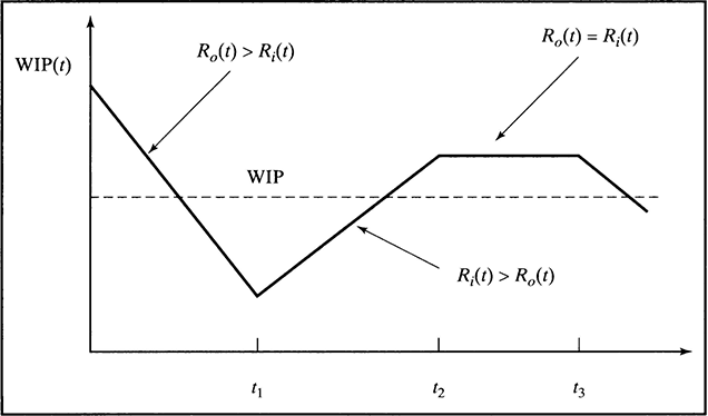
FIGURE 5.2 Work-in-Process Level over Time
5.1.3 CYCLE TIME
Cycle time (also known as throughput time) is one of the most important measures of performance of a business process. This value is frequently the main focus when comparing the performance of alternative process designs. The cycle time is the time that it takes to complete an individual job from start to finish. In other words, it is the time that it takes for a job to go from the entry point to the exit point of a process. This is the time that a customer experiences. For example, the cycle time at a bank may be the time that elapses from the instant a customer enters the facility until the same customer leaves. In an Internet ordering process, cycle time may be the time elapsed from the time a customer places an order until the order is received at home. Because jobs follow different routings in a process, the cycle time can be considerably different from job to job. For example, some jobs might have a routing through a set of activities performed by resources with large capacity and, therefore, would not have to wait to be processed, resulting in shorter cycle times. On the other hand, long cycle times can be the result of jobs having to compete for scarce resources.
The cycle time of any given job is the difference between its departure time from the process and its arrival time to the process. If a customer joins a queue in the post office at 7:43 A.M. and leaves at 7:59 A.M., the customer’s cycle time is 16 minutes. The average cycle time (CT) is the sum of the individual cycle times associated with a set of jobs divided by the total number of jobs4. The cycle time depends not only on the arrival rate of jobs in a given time period but also on the routing and the availability of resources.
Because the cycle time is the total time a job spends in the process, the cycle time includes the time associated with value-adding and non-value-adding activities. The cycle time typically includes:
- Processing time,
- Inspection time,
- Transportation time,
- Storage time,
- Waiting time (planned and unplanned delay time).
Processing time is often related to value-adding activities. However, in many cases, the processing time is only a small fraction of the cycle time. Cycle time analysis is a valuable tool for identifying opportunities to improve process performance. For example, if an insurance company finds out that it takes 100 days (on average) to process a new commercial account and that the actual processing time is only about 2 days, then there might be an opportunity for a significant process improvement with respect to cycle time.
5.1.4 LITTLE’S LAW
A fundamental relationship between throughput, work-in-process, and cycle time is known as Little’s law. J. D. C. Little proposed a proof for this formula in connection with queuing theory (Little, 1961). The relationship, which has been shown to hold for a wide class of queuing situations, is:
The formula states that the average number of jobs in the process is proportional to the average time that a job spends in the process, where the factor of proportionality is the average arrival rate. Little’s law refers to the average (or expected) behavior of a process. The formula indicates that if two of the three operational measures can be managed (that is, their values are determined by conscious managerial decisions), the value of the third measure is also completely determined. Three basic relationships can be inferred from Little’s law.
- Work-in-process increases if the throughput rate or the cycle time increases.
- The throughput rate increases if work-in-process increases or cycle time decreases.
- Cycle time increases if work-in-process increases or the throughput rate decreases.
These relationships must be interpreted carefully. For example, is it true that in an order-fulfillment process, more work-in-process inventory results in an increase of cycle time? Most people would argue that higher levels of inventory (either of finished product or of work-in-process) should result in a shorter cycle time, because the order can be filled faster when the product is finished (or in the process to be finished) than when it has to be produced from scratch. Is Little’s law contradicting common sense? The answer is no. A closer examination of the order-fulfillment process reveals that there are, in fact, two work-in-process inventories: one associated with purchasing orders and the other with products. In this case, Little’s law applies only to the work-in-process inventory of orders and not to the inventory of products. Now it is reasonable to state that if the number of orders in the pipeline (i.e., the work-in-process inventory of orders) increases, the cycle time experienced by the customer also increases.
Finally, some companies use a performance measure known as inventory turns or turnover ratio. If WIP is the number of jobs in a process at any point in time, then the turnover ratio indicates how often the WIP is replaced in its entirety by a new set of jobs. The turnover ratio is simply the reciprocal of the cycle time; that is:
Example 5.2
An insurance company processes an average of 12,000 claims per year. Management has found that on average, at any one time, 600 applications are at various stages of processing (e.g., waiting for additional information from the customer, in transit from the branch office to the main office, waiting for an authorization, and so on). If it is assumed that a year includes 50 working weeks, how many weeks (on the average) does processing a claim take?

Little’s law indicates that the average cycle time for this claim process is 2.5 weeks. Suppose management does not consider this cycle time acceptable (because customers have been complaining that the company takes too long to process their claims). What options does management have to reduce the cycle time to, say, 1 week? According to Little’s law, in order to reduce the cycle time, either the work-in-process must be reduced or the throughput rate must be increased.
A process redesign project is conducted, and it is found that most claims experience long, unplanned delays (e.g., waiting for more information). The new process is able to minimize or eliminate most of the unplanned delays, reducing the average work-in-process by half. The cycle time for the redesigned process is then:
5.2 Cycle Time and Capacity Analysis
In this section, the concepts of cycle time, throughput, and work-in-process inventory are used along with Little’s law to analyze the capacity of processes. A process is still viewed as a set of activities that transforms inputs into outputs. Jobs are routed through a process, and resources perform the activities. The routing of jobs and the possibility of rework affect cycle time, and the amount of resources and their capabilities affect process capacity.
5.2.1 CYCLE TIME ANALYSIS
Cycle time analysis refers to the task of calculating the average cycle time for an entire process or a process segment. The cycle time calculation assumes that the time to complete each activity is available. The activity times are average values and include waiting time (planned and unplanned delays). Flow diagrams are used to analyze cycle times, assuming that only one type of job is being processed. In the simplest case, a process may consist of a sequence of activities with a single path from an entry point to an exit point. In this case, the cycle time is simply the sum of the activity times. However, not all processes have such a trivial configuration. Therefore, the cycle time analysis needs to be considered in the presence of rework, multiple paths, and parallel activities.
Rework
An important consideration when analyzing cycle times relates to the possibility of rework. Many processes use control activities to monitor the quality of the work. These control activities (or inspection points) often use specified criteria to allow a job to continue processing. That is, the inspection points act as an accept/reject mechanism. The rejected jobs are sent back for further processing, affecting the average cycle time and ultimately the capacity of the process (as will be discussed in the next section).
Example 5.3
Figure 5.3 shows the effect of rework on the average cycle time of a process segment. In this example, it is assumed that each activity (i.e., receiving the request and filling out parts I and II of the order form) requires 10 minutes (as indicated by the number between parentheses) and that the inspection (the decision symbol labeled “Errors?”) is done in 4 minutes on the average. The jobs are processed sequentially through the first three activities, and then the jobs are inspected for errors. The inspection rejects an average of 25 percent of the jobs. Rejected jobs must be reworked through the last two activities associated with filling in the information in the order form.
Without the rework, the cycle time of this process segment from the entry point (i.e., receiving the request) to the exit point (out of the inspection activity) is 34 minutes; that is, the sum of the activity times and the inspection time. Because 25 percent of the jobs are rejected and must be processed through the activities that fill out the order form as well as being inspected once more, the cycle time increases by 6 minutes (24 × 0.25) to a total of 40 minutes on the average. In this case, the assumption is that jobs are rejected only one time.

If it is assumed that the rejection percentage after the inspection in a rework loop is given by r, and that the sum of the times of activities within the loop (including inspection) is given by T, then the following general formula can be used to calculate the cycle time from the entry point to the exit point of the rework loop.
This formula assumes that the rework is done only once. That is, it assumes that the probability of an error after the first rejection goes down to zero. If the probability of making an error after an inspection remains the same, then the cycle time through the rework loop can be calculated as follows.

In Example 5.3, the average cycle time for the entire process would be calculated as follows, taking into consideration that the probability of an error remains at 25 percent regardless of the number of times the job has been inspected:
Multiple Paths
In addition to rework, a process might include routings that create separate paths for jobs after specified decision points. For example, a process might have a decision point that splits jobs into “fast track” and “normal track.” In this case, a percentage must be given to indicate the fraction of jobs that follow each path.
Example 5.4
Figure 5.4 shows a flowchart of the process for Speedy Tax Services described in Example 5.1. All clients are received by the receptionist, after which a decision is made to send a fraction of the clients to a professional tax specialist and the remaining clients to a tax preparation associate. On the average, 70 percent of the clients have complicated tax returns and need to work with a professional tax specialist. The remaining 30 percent of the clients have simple tax returns and can be helped by tax preparation associates. The numbers between parentheses associated with each activity indicate the activity time (in minutes). With this information, the average cycle time associated with this process can be calculated. In this case, the cycle time represents the average time that it takes for a client to complete his or her tax return and pay for the service.
The cycle time calculation in Figure 5.4 represents the sum of the contribution of each activity time to the total. All clients are received by a receptionist, so the contribution of this activity to the total cycle time is 5 minutes. Similarly, the contribution of the last activity to the cycle time is 6 minutes, given that all clients must pay before leaving the facility. The contribution of the other two activities in the process is weighted by the percentage of clients that are routed through each of the two paths.

A general formula can be derived for a process with multiple paths. Assume that m paths originate from a decision point. Also assume that the probability that a job follows path i is pi and that the sum of activity times in path i is Ti. Then the average cycle time across all paths is given by:
Parallel Activities
Cycle time analysis also should contemplate routings in which activities are performed in parallel. For example, a technician in a hospital can set up the X-ray machine for a particular type of shot (as required by a physician), while the patient prepares (e.g., undresses). These two activities occur in parallel, because it is not necessary for the technician to wait until the patient is ready before starting to set up the X-ray machine. Because one of these activities will require less time, the other has to wait for further processing. Typically, the patient will finish first and will wait to be called for the X ray. The contribution to the cycle time is then given by the maximum time from all the parallel activities.
Example 5.5
Figure 5.5 depicts a process with five activities. The first activity consists of opening an envelope and splitting its contents into three different items: application, references, and credit history. Each of these items is processed in parallel, and a decision is made regarding this request after the parallel activities have been completed. The numbers between parentheses in Figure 5.5 are activity times in minutes.
The cycle time calculation in Figure 5.5 results in a total of 40 minutes for the process under consideration. This is the sum of 5 minutes for the first activity, 20 minutes for checking the credit history (which is the parallel activity with the longest time), and 15 minutes for making a decision. Note that the flow diagram in Figure 5.5 has no decision point after the first activity, because all the jobs are split in the same way; that is, the routing of all the jobs is the same and includes the parallel processing of the “checking” activities. Note also that these are considered inspection activities, and therefore the square is used to represent them in the flowchart in Figure 5.5.

The general formula for process segments with parallel activities is a simplification of the one associated with multiple paths. Because there is no decision point when the jobs are split, it is not necessary to account for probability values. It is assumed that Ti is the total time of the activities in path i (after the split) and that the process splits into m parallel paths. Then the cycle time for the process segment with parallel paths is given by:
Example 5.6
Before concluding this section, let us apply the aforementioned principles for cycle time analysis to a small process. Assume that a process has been described and that the flow diagram in Figure 5.6 was drawn appropriately from these descriptions. The numbers in paranthesis shown in Figure 5.6 are activity times in minutes. The process consists of nine activities. A decision point is included after activity A, because only 30 percent of the jobs are required to go through activity B. A rework loop sends jobs back from the inspection point I to activity D. This loop assumes that the reworked jobs are examined a second time and that they always pass the inspection; that is, jobs are reworked only one time. The process has two parallel activities, F and G, before the last activity is performed.
The cycle time calculation that corresponds to the process in Figure 5.6 starts with the time for activity A. Next, the contribution of 6 minutes (i.e., 0.3 × 20) from activity B is added. This is followed by the time of activity C (23 minutes) and the contribution of the activities in the rework loop. Note that the times within the rework loop are added, including the inspection time, and multiplied by 110 percent. This operation accounts for the 10 percent of jobs that are sent back after inspection. Finally, the contribution of the parallel activities is calculated as the maximum time between activity F and G, followed by the activity time for H. The average cycle time for this process is determined to be 92.5 minutes.

After calculating the cycle time of a process, the analyst should calculate what is known as the cycle time efficiency. Assuming that all processing times are value adding, the cycle time efficiency indicates the percentage of time, from the actual cycle time, that is spent performing value-adding work. Mathematically, the cycle time efficiency is expressed as follows.
Process time also is referred to as the theoretical cycle time, because theoretically a job can be completed in that time (that is, if no waiting would occur). To calculate the process time, replace activity time with the processing time (i.e., the activity time minus the waiting time). It should be recognized that the cycle time efficiency calculated here is conceptually the same as the efficiency calculation in Chapter 4, which was connected with line balancing.
Example 5.7
Table 5.1 shows the time values associated with the activities in Example 5.6. The time values are broken down into processing time and waiting time. The activity time is the sum of these two values.
Using the processing times in Table 5.1 and the flow diagram in Figure 5.6, the process time ( or theoretical cycle time) can be calculated as follows.
The cycle time efficiency can now be found as follows.
This means that less than one third of the actual cycle time is spent in processing, and the rest of the time is spent waiting.
TABLE 5.1 Activity Times for Example 5.7

Redesign projects in several industries (e.g., insurance, hospitals, and banking) indicate that it is not unusual to find cycle time efficiencies of less than 5 percent. This occurs, for example, in applications for a new insurance policy, where the process time is typically 7 minutes and the cycle time is normally 72 hours.
5.2.2 CAPACITY ANALYSIS
Capacity analysis complements the information obtained from a cycle time analysis when studying flows in a process. Flowcharts are important also for analyzing capacity, because the first step in the methodology consists of estimating the number of jobs that flow through each activity. This step is necessary because resources (or pools of resources) perform the activities in the process, and their availability limits the overall capacity. The number of jobs flowing through each activity is determined by the configuration of the process, which may include, as in the case of the cycle time analysis, rework, multiple paths, and parallel activities.
Rework
When a process or process segment has a rework loop, the number of jobs flowing through each activity varies according to the rejection rate.
Example 5.8
Figure 5.7 depicts a process with a rework loop. Requests are processed through three activities and then inspected for errors. Suppose 100 requests are received. Because an average of 25 percent of the requests are rejected, the second and third activities, which are inside the rework loop, end up processing 125 jobs in the long run. This is assuming that rejected requests always pass inspection the second time.

FIGURE 5.7 Number of Requests Flowing Through Each Activity in a Process with Rework
Next, a general formula is derived for calculating the number of jobs per activity in a rework loop. Assume that n jobs enter the rework loop and that the probability of rejecting a job at the inspection station is r. The number of jobs flowing through each activity in the loop, including the inspection station, is given by the following equation.
When the rejection rate stays the same regardless of the number of times that a job has been reworked and inspected, then the number of jobs that are processed by activities inside the rework loop is given by the following equation.
According to this formula, the activities inside the rework loop in Example 5.8 (see Figure 5.7) process 133.33 requests on the average.
Multiple Paths
The job routings in a process may include decision points that create multiple paths. The flow through each path varies according to the frequency with which each path is selected (as indicated in the decision point).
Example 5.9
Figure 5.8 shows a flowchart of the process for Speedy Tax Services described in Example 5.1, which contains multiple paths. Assume that 100 clients enter the process, and we want to calculate the number of clients that are processed at each activity on the average.
Because 30 percent of the clients have simple tax returns, about 30 clients out of 100 are helped by tax preparation associates. On the average, the remaining 70 clients are helped by professional tax specialists. It is important to note that all 100 clients must pay for the services rendered, so they are routed through the cashiers.

FIGURE 5.8 Number of Clients Flowing Through Each Activity in a Process with Multiple Paths
To derive a general formula for the number of jobs in each path, assume that the probability that a job follows path i is pi. Also assume that n jobs enter the decision point. Then, the number of jobs in path i is given by the following equation.
Parallel Activities
When jobs split into parallel activities, the number of jobs flowing through each activity remains the same as the number of jobs that enter the process (or process segment).
Example 5.10
Figure 5.9 shows a process with five activities, three of which are performed in parallel. Assuming that 100 applications are received, all activities experience the same load of 100 applications, as shown in Figure 5.9.

FIGURE 5.9 Number of Applications Flowing Through Each Activity in a Process with Parallel Activities
In this case, no general formula is necessary, because the number of jobs remains the same after a split into parallel activities or paths. The next step in analyzing capacity is to determine the capacity of each resource or pool of resources. This calculation is illustrated using the process of Example 5.6, whose flowchart is depicted in Figure 5.6.
Example 5.11
For each activity in the process, the processing time, the type of resource required, and the number of jobs processed through each activity must be known. This information is summarized in Table 5.2.
The available resources of each type also must be known. Table 5.2 indicates that there are three types of resources, labeled Rl, R2, and R3. Assume that there are two units of resource Rl, two units of resource R2, and one unit of resource R3.
TABLE 5.2 Resource Capacity Data for Example 5.11

TABLE 5.3 Pool Capacity Calculation for Example 5.11

The resource unit and pool capacity can now be calculated as follows. For each resource type, find the unit load. To calculate the unit load for a given resource, first multiply the processing time by the number of jobs for each activity for which the resource is required, and then add the products. This is illustrated in the second column of Table 5.3. The unit capacity for each resource is the reciprocal of the unit load and indicates the number of jobs that each unit of resource can complete per unit of time. This is shown in the third column of Table 5.3.
Finally, to find the pool capacity associated with each resource type, multiply the number of resource units (i.e., the resource availability) by the unit capacity. The values corresponding to resources Rl, R2, and R3 are shown in column 5 of Table 5.3 (labeled Pool Capacity).
The pool capacities in Table 5.3 indicate that resource R2 is the bottleneck of the process, because this resource type has the smallest pool capacity. The pool capacity of R2 is 0.13 jobs per minute or 7.8 jobs per hour, compared to 0.36 jobs per minute or 21.6 jobs per hour for Rl and 0.17 jobs per minute or 10.2 jobs per hour for R3.
It is important to realize that the bottleneck of a process refers to a resource or resource pool and not to an activity. In other words, capacity is not associated with activities but with resources. Also note that because the slowest resource pool limits the throughput rate of the process, the process capacity is determined by the capacity of the bottleneck. Therefore, the capacity of the process depicted in Figure 5.6 is 7.8 jobs per hour.
The process capacity, as previously calculated, is based on processing times instead of activity times. Because processing times do not include waiting time, the process capacity calculation is a value that can be achieved only in theory. That is, if jobs are processed without any delays (either planned or unplanned), the process can achieve its theoretical capacity of 7.8 jobs per hour. In all likelihood, however, the process actual throughput rate (or actual capacity) will not match the theoretical process capacity; therefore, a measure of efficiency can be calculated. The measure in this case is known as the capacity utilization, and it is defined as follows.

With this mathematical relationship, the capacity utilization can be calculated for each resource type in a process.
Example 5.12
Assume that the throughput rate of the process in Example 5.11 is six jobs per hour. This additional piece of information gives the following capacity utilization values for each resource in the process.

Similar to the way the capacity of the process is related to the capacity of the bottleneck resource, the capacity utilization of the process is related to the capacity utilization at the bottleneck. Thus, based on the calculations in Example 5.12 the capacity utilization of the process in Example 5.11 is 76.9 percent.
5.3 Managing Cycle Time and Capacity
The analysis of cycle time and capacity provides process managers with valuable information about the performance of the process. This information, however, is wasted if managers do not translate it into action. Through cycle time analysis, managers and process designers can find out the cycle time efficiency of the process and discover, for example, that the waiting time in the process is excessive for a desired level of customer service. This section discusses ways to reduce cycle time and strategies to increase capacity.
5.3.1 CYCLE TIME REDUCTION
Process cycle time can be reduced in five fundamental ways.
- Eliminate activities.
- Reduce waiting time.
- Eliminate rework.
- Perform activities in parallel.
- Move processing time to a noncritical activity.
The first thing that analysts of business processes should consider is the elimination of activities. As discussed in earlier chapters, most of the activities in a process do not add value to the customer; therefore, they should be considered for elimination. Non-value-adding activities, such as those discussed in Chapter 1, increase the cycle time but are not essential to the process.
If an activity cannot be eliminated, then eliminating or minimizing the waiting time reduces the activity time. Recall that the activity time is the sum of the processing time and the waiting time. It is worth investigating ways to speed up the processing of jobs at an activity, but larger time reductions are generally easier to achieve when waiting time is eliminated. Waiting time can be reduced, for example, by decreasing batch sizes and set up times. Also, improved job scheduling typically results in less waiting and better utilization of resources.
Example 5.3 shows that rework loops add a significant amount of time to the process cycle time. As shown in that example, the cycle time when the activities are performed “right” the first time, and thus eliminating the need for the rework loop, is 85 percent (or 34/40) of the original cycle time. If the jobs always pass inspection, the inspection activity also can be eliminated, reducing the cycle time to 30 minutes. This represents a 25 percent reduction from the original design.
Changing a process design to perform activities in parallel has an immediate impact on the process cycle time. This was discussed in Chapter 4, where the notion of combining activities was introduced. (Recall that the combination of activities is the cornerstone of the process design principle known as case management, as described in Chapter 3.) Mathematically, the reduction of cycle time from a serial process configuration to a parallel process configuration is the difference between the sum of the activity times and the maximum of the activity times. To illustrate, suppose that the “checking” activities in Figure 5.5 were performed in series instead of in parallel. The average cycle time for completing one application becomes:
The cycle time with parallel processing was calculated to be 40 minutes. The difference of 32 minutes also can be calculated as follows.
Finally, cycle time decreases when some work content (or processing time) is shifted from a critical activity to a noncritical activity. In a process with parallel processing (i.e., with a set of activities performed in parallel), the longest path (in terms of time) is referred to as the critical path. The length of the critical path corresponds to the cycle time of the process.
Example 5.13
Consider, for instance, the activities depicted in Figure 5.5. This process has three paths.
| Path | Length |
|---|---|
| Receive → Check Application → Decide | 5 + 14 + 15 = 34 minutes |
| Receive → Check Credit → Decide | 5 + 20 + 15 = 40 minutes |
| Receive → Check References → Decide | 5 + 18 + 15 = 38 minutes |
The longest path is the second one with a length of 40 minutes.
Then the critical activities are Receive, Check Credit, and Decide, and the path length of 40 minutes matches the cycle time calculated in Figure 5.5.
Example 5.14
Figure 5.10 depicts a process with six activities. In this process, activities C and D are performed in parallel along with activity E. Assume that the numbers between parentheses are activity times. The process has two paths.
| Path | Length |
|---|---|
| A→ B→ C→ D→ F | 10 + 20 + 15 + 5 + 10 = 60 minutes |
| A → B → E → F | 10 + 20 + 12 + 10 = 52 minutes |

FIGURE 5.10 Original Process in Example 5.14
The critical activities in the original process are A, B, C, D, and F. These activities belong to the critical path. In order to reduce cycle time, a redesigned process might move some work from a critical activity to a noncritical activity. In this case, activity E is the only noncritical activity. Suppose it is possible to move 4 minutes of work from activity C to activity E. This change effectively reduces the cycle time by 4 minutes, making both paths critical. That is, both paths of activities in the process now have the same length of 56 minutes; therefore, all the activities in the process have become critical. Note also that in the following calculation of the cycle time, both of the time values compared in the “max” function equal 16 minutes.
We next examine ways to increase process capacity.
5.3.2 INCREASING PROCESS CAPACITY
Section 5.2.2 examined the direct relationship between process capacity and the capacity of the bottleneck resource. Given this relationship, it is reasonable to conclude that making the bottleneck resource faster results in an increase of process capacity. Capacity of the process can be increased in two fundamental ways.
- Add resource availability at the bottleneck.
- Reduce the workload at the bottleneck.
Adding resources to the bottleneck might mean additional investment in equipment and labor or additional working hours (i.e., overtime). In other words, the available resources at the bottleneck can be increased with either more workers or with the same workers working more hours.
The approach of reducing workload at the bottleneck is more closely linked to the notion of process redesign. The reduction consists of either shifting activities from the bottleneck to a different resource pool or reducing the time of the activities currently assigned to the bottleneck. Shifting activities from one resource pool to another requires cross training so that workers in a nonbottleneck resource pool can perform new activities.
One must be careful when considering redesign strategies with the goal of reducing cycle time and increasing process capacity. Specifically, the decision must take into consideration the availability of resources and the assignment of activities to each resource pool.
Example 5.15
Assume that five resource types are associated with the process in Figure 5.10. Also assume that each type of resource has only one available unit. Finally, assume that activities A, B, C, and D are assigned to resources Rl, R2, R3, and R4, respectively, and that activities E and F areassigned to resource R5. Given these assignments and assuming, for simplicitly, that for all activities the processing times equals the activity times in Figure 5.10, the theoretical capacity of the original process can be calculated as shown in Table 5.4.
TABLE 5.4 Capacity of the Original Process

The bottleneck is resource R5 with a capacity of 2.7 jobs per hour, which also becomes the process capacity. The cycle time for this process was calculated to be 60 minutes.
If the process is modified in such a way that 4 minutes of work are transferred from activity C to activity E, then, as shown in Example 5.14, the cycle time is reduced to 56 minutes. Does the process capacity change as a result of this process modification? Table 5.5 shows the process capacity calculations associated with the modified process.
TABLE 5.5 Capacity of the Modified Process

The calculations in Table 5.5 indicate that the process capacity decreases as a result of the decision to transfer units from a critical activity to a noncritical activity associated with the bottleneck resource R5. At first glance, this result seems to contradict Little’s law, which specifies that the throughput rate increases when cycle time decreases. In this case, cycle timedecreased from 60 minutes to 56 minutes, and the process capacity (measured in units of throughput) decreased from 2.7 jobs/hour to 2.3 jobs/hour.
The change in the level of work-in-process explains this apparent contradiction. Although it is true that a shorter cycle time should increase the throughput rate, this holds only if the work-in-process remains unchanged. In this example, the decision to move processing time from activity C to activity E decreases cycle time and throughput rate, and as a result also decreases the work-in-process.
5.4 Theory of Constraints
Bottlenecks affect the efficiency of processes because they limit throughput, and in many cases they also inhibit the achievement of value-based goals, such as quality, speed, cost, and flexibility. Bottlenecks often are responsible for the differences between what operation managers promise and what they deliver to internal and external customers (Melnyk and Swink, 2002). Due to the importance of bottlenecks, it is not sufficient to be able to identify their existence. That is, locating the bottlenecks in a process is just part of managing flows; the other part deals with increasing process efficiency despite these limitations. This section introduces a technique for managing bottlenecks that is known as theory of constraints.
Theory of constraints (TOC) provides a broad theoretical framework for managing flows. It emphasizes the need for identifying bottlenecks (or constraints) within a process, the entire firm, or even the business context. For example, an organization’s information system represents a constraint if the order-entry function takes longer to prepare an order for release than the transformation process needs to make the product. Other constraints could be associated with resources that perform activities in areas such as marketing, product design and development, or purchasing. All of these constraints limit throughput and, therefore, affect the efficiency of the system.
As mentioned in Chapter 4, TOC draws extensively from the work of Eli Goldratt, an Israeli physicist. TOC leads to an operating philosophy that in some ways is similar to just-in-time5. TOC assumes that the goal of a business organization is to make money. To achieve this goal, the company must focus on throughput, inventory, and operating expenses. In order to increase profit, a company must increase throughput and decrease inventory and operating expenses. Then, companies must identify operations policies that translate into actions that move these variables in the right directions. However, these policies have to live within a set of relevant constraints.
Theory of constraints gets its name from the concept that a constraint is anything that prevents a system from achieving higher levels of performance relative to its goal (Vonderembse and White, 1994). Consider the following situations where decisions must be made in constrained settings.
Example 5.16
A company produces products A and B using the same process. The unit profit for product A is $80, and the market demand is 100 units per week. The unit profit for product B is $50, and the market demand is 200 units per week. The process requires 0.4 hours to produce one unit of A and 0.2 hours to produce one unit of B. The process is available 60 hours per week. Because of this constraint, the process is unable to meet the entire demand for both products. Consequently, the company must decide how many products of each type to make. This situation is generally known as the product-mix problem.
If the objective of the company is to maximize total profit, one would be inclined to recommend the largest possible production of A, because this product has the largest profit margin. This production plan can be evaluated as follows. First, calculate the maximum number of units of A that can be produced in 60 hours of work.
Although 150 units can be produced per week, the market demands only 100. Therefore, the production plan would recommend 100 units of A. Because producing 100 units of A requires 40 hours of process time (i.e., 0.4 × 100), then 20 hours are still available to produce product B. This process time translates into 100 units of product B (i.e., 20/0.2). The total profit associated with this production plan is:
Is this the best production plan? That is, does this production plan maximize weekly profits? To answer this question, first examine an alternative plan. If the company first attempts to meet the demand for product B, then the required process time would be 40 hours (i.e., 200 × 0.2). This would leave 20 hours to produce product A, resulting in 50 units (i.e., 20/0.4). The total profit associated with this plan would be:
The alternative plan increases total profit by $1,000 per week. This example shows that when constraints are present, decisions cannot be made using simplistic rules. In this case, we attempted to solve the problem by simply maximizing the production of the product with the largest profit margin. This solution, however, takes into consideration neither the production constraints nor the market demand constraints.
Example 5.17
A department store chain has hired an advertising firm to determine the types and amounts of advertising it should have for its stores. The three types of advertising available are radio and television commercials and newspaper ads. The retail chain desires to know the number of each type of advertisement it should pursue in order to maximize exposure. It has been estimated that each ad or commercial will reach the potential audience shown in Table 5.6. This table also shows the cost associated with each type of advertisement.
TABLE 5.6 Advertising Data

In order to make a decision, the company must consider the following constraints.
- The budget limit for advertisement is $100,000.
- The television station has time available for four commercials.
- The radio station has time available for 10 commercials.
- The newspaper has space available for seven ads.
- The advertising agency has time and staff available for producing no more than a total of 15 commercials and/or ads.
The company would like to know how many and what kinds of commercials and ads to produce in order to maximize total exposure. If one follows the simple criterion of choosing advertising by its exposure potential, one would try to maximize TV commercials, then radio commercials, and finally newspaper ads. This would result in four TV commercials ($60,000), six radio commercials ($36,000) and one newspaper ad ($4,000). The cost of the campaign would be $100,000 with an estimated exposure of 161,000 people. This problem, however, can be formulated as an integer programming6 model and optimally solved, for instance, with Microsoft Excel’s Solver. The optimal solution to this problem calls for two TV commercials, nine radio commercials, and four newspaper ads for a total cost of $100,000 and a total exposure of 184,000 people.
This example shows, once again, that simplistic solutions to constrained problems can lead to inferior process performance. In this case, a more comprehensive solution method is able to increase by 14 percent the total exposure that can be achieved with a fixed amount of money.
Examples 5.16 and 5.17 include constraints associated with production, demand, and capacity. In general, constraints fall into three broad categories.
Resource constraint: A resource within or outside the organization, such as capacity, that limits performance.
Market constraint: A limit in the market demand that is less than the organization’s capacity.
Policy constraint: Any policy that limits performance, such as a policy that forbids the use of overtime.
In Examples 5.16 and 5.17, the limit in the process hours and the budget for advertising can be identified as resource constraints. An external resource constraint is the limit on the number of ads or commercials the advertising agency is able to produce for the discount stores. The market constraint in Example 5.16 is characterized by a limit on the weekly demand for each product. One possible policy constraint in Example 5.17 might be to insist on a plan whereby the number of TV commercials is greater than the number of newspaper ads.
TOC proposes a series of steps that can be followed to deal with any type of constraint (Vonderembse and White, 1994).
- Identify the system’s constraints.
- Determine how to exploit the system constraints.
- Subordinate everything else to the decisions made in step 2.
- Elevate the constraints so a higher performance level can be reached.
- If the constraints are eliminated in step 4, go back to step 1. Do not let inertia become the new constraint.
Example 5.18
We now apply the first three steps of this methodology to a process with nine activities and three resource types. Three types of jobs must be processed, with each job following a different processing path. The routing for each job, the weekly demand, and the estimated profit margins are shown in Table 5.7.
To make the analysis for this example simple, assume that activities 1, 2, and 3 require 10 minutes and that the other activities require 5 minutes of processing for each job. Also, assume that activities 1, 2, and 3 are performed by resource X; activities 4, 5, and 6 are performed by resource Y; and activities 7, 8, and 9 are performed by resource Z. Finally, assume that 2,400 minutes of each resource are available per week.
- Identify the system’s constraints. This problem has two types of constraints: a resource constraint and a market constraint. The resource constraint is given by the limit on the processing time per week. The market constraint is given by the limit on the demand for each job. Next, identify which one of these two types of constraints is restricting the performance of the process. Table 5.8 shows the resource utilization calculations if the process were to meet the market demands. That is, these calculations assume that 50 A jobs, 100 B jobs, and 60 C jobs will be processed per week.
The requirement calculations in Table 5.8 reflect the total time needed by each job type per resource. For example, resource Y performs activities 4, 5, and 6. Because 50 A jobs are routed through activity 4 and the activity time is 5 minutes, this requires 5 × 50 = 250 minutes of resource Y per week. Then 100 B jobs are routed through activities 5 and 6, adding 10 × 100 = 1,000 minutes to resource Y. Finally, 60 C jobs are routed through activities 4, 5, and 6, resulting in 15 × 60 = 900 additional minutes of resource Y. Hence, the process requires 2,150 minutes of resource Y per week. Because 2,400 minutes are available, the utilization of resource Y is 2,150/2,400 = 90 percent. The utilization of resources X and Z are obtained in the same manner.
TABLE 5.7 Job Data for Example 5.17

TABLE 5.8 Utilization Calculations for Example 5.17

In order to meet market demand, resource X is required at more than 100% utilization, so clearly the process is constrained by this resource.
- Determine how to exploit the system's constraint. Next, determine how resource X can be utilized most effectively. Let us consider three different rules to process jobs, and for each rule, calculate the total weekly profit.
- 2.1 Rank jobs based on profit margin. This rule would recommend processing jobs in the order given by B, C, and A.
- 2.2 Rank jobs based on their profit contribution per direct labor hour. These contributions are calculated as the ratio of profit and total direct labor. For example, job A has a contribution of $1.33 per direct labor minute, because its profit margin of $20 is divided by the total labor of 15 minutes (i.e., $20/15 = $1.33). Similarly, the contributions of B and C are $1.50 and $1.20, respectively. These calculations yield the processing order of B, A, and C.
- 2.3 Rank jobs based on their contribution per minute of the constraint. These contributions are calculated as the ratio of profit and direct labor in resource X (i.e., the bottleneck). For example, job B has a contribution of $2.50 per direct labor minute in resource X, because its profit margin of $75 is divided by the total labor of 30 minutes in resource X (i.e., $75/30 = $2.50). Similarly, the contribution of C is $3.00. The contribution of A in this case is irrelevant, because A jobs are not routed through any activities requiring the bottleneck resource X. The rank is then C and B, with A as a “free” job with respect to the constraint.
- Subordinate everything else to the decisions made in step 2. This step involves calculating the number of jobs of each type to be processed, the utilization of each resource, and the total weekly profit. These calculations depend on the ranking rule used in step 2, so the results of using each of the proposed rules are shown as follows.
- 3.1 Start by calculating the maximum number of jobs of each type that can be completed using ranking rule 2.1. The maximum number of B jobs is 80 per week, which is the maximum that resource X can complete (i.e., 2,400/30 = 80). If 80 B jobs are processed, then no C jobs can be processed, because no capacity is left in resource X. However, type A jobs can be processed, because they don’t use resource X. These jobs use resources Y and Z. Resource Y does not represent a constraint, because its maximum utilization is 90 percent (as shown in Table 5.8). After processing B jobs, 1,600 minutes are left in resource Z (i.e., 2,400 − 800). Each A job requires 10 minutes of resource Z, so a maximum of 1,600/10 = 160 A jobs can be processed. Given that the demand is 50 A jobs per week, the entire demand can be satisfied. The utilization of each resource according to this plan is shown in Table 5.9.
The total profit of this processing plan is $75 × 80 + $20 54 × 50 = $7,000.
- 3.2 The ranking according to rule 2.2 is B, A, and C. Because A does not require resource X, the resulting processing plan is the same as the one for rule 2.1 (see Table 5.9). The total profit is also $7,000.
- 3.3 For the ranking determined by rule 2.3, first calculate the maximum number of C jobs that can be processed through the bottleneck. C jobs require 20 minutes of resource X, so a total of 120 C jobs can be processed per week (i.e., 2,400/20 = 120). This allows for the entire demand of 60 C jobs to be satisfied. Now, subtract the capacity from the bottleneck and calculate the maximum number of B jobs that can be processed with the remaining capacity. This yields 1,200/30 = 40 B jobs. Finally, the number of A jobs that can be processed is calculated. A jobs are “free” with respect to resource X but require 10 minutes of processing in resource Z. The updated capacity of resource Z is 1,300 minutes (after subtracting 400 minutes for B jobs and 900 minutes for C jobs); therefore, the entire demand of A jobs can be satisfied. The utilization of the resulting plan is given in Table 5.10.
TABLE 5.10 Utilization for Ranking Rule 2.3

The total profit of this processing plan is $20 54 × 50 + $75 54 × 40 + $60 54 × 60 = $7,600.
- 3.1 Start by calculating the maximum number of jobs of each type that can be completed using ranking rule 2.1. The maximum number of B jobs is 80 per week, which is the maximum that resource X can complete (i.e., 2,400/30 = 80). If 80 B jobs are processed, then no C jobs can be processed, because no capacity is left in resource X. However, type A jobs can be processed, because they don’t use resource X. These jobs use resources Y and Z. Resource Y does not represent a constraint, because its maximum utilization is 90 percent (as shown in Table 5.8). After processing B jobs, 1,600 minutes are left in resource Z (i.e., 2,400 − 800). Each A job requires 10 minutes of resource Z, so a maximum of 1,600/10 = 160 A jobs can be processed. Given that the demand is 50 A jobs per week, the entire demand can be satisfied. The utilization of each resource according to this plan is shown in Table 5.9.

Rule 2.3 yields superior results in constrained processes where the goal is selecting the mix of products or services that maximizes total profit. Therefore, it is not necessary to apply rules 2.1 and 2.2 in these situations, because their limitations have been shown by way of the previous example. The application of rule 2.3 to the production and marketing examples (Examples 5.16 and 5.17) presented earlier in this section is left as exercises.
5.5 Summary
This chapter has discussed two important aspects in the modeling and design of business processes: cycle time analysis and capacity analysis. Cycle time analysis represents the customer perspective because most customers are concerned with the time that they will have to wait until their jobs are completed. Market demands are such that business processes must be able to compete in speed in addition to quality and other dimensions of customer service.
On the other hand, operations managers are concerned with the efficient utilization of resources. Capacity analysis represents this point of view. Competitive processes are effective at balancing customer service and resource utilization. The techniques for managing flow discussed in this chapter are relevant in the search for the right balance.
5.6 References
Anupindi, R., S. Chopra, S. D. Deshmukh, J. A. Van Mieghem, and E. Zemel. 1999. Managing business process flows. Upper Saddle River, NJ: Prentice Hall.
Finch, B. J., and R. L. Luebbe. 1995. Operations management: Competing in a changing environment. Fort Worth, TX: Dryden Press.
Little, J. D. C. 1961. A proof of the queuing formula L = λW. Operations Research 9: 383–387.
Melnyk, S., and M. Swink. 2002. Value-driven operations management: An integrated modular approach. New York: McGraw Hill/Irwin.
Sterman, J. D. 2000. Business dynamics: Systems thinking and modeling for a complex world. Boston: Irwin McGraw-Hill.
Vonderembse, M. A., and G. P. White. 1994. Operations management: Concepts, methods, and strategies. Ontario: John Wiley & Sons Canada Ltd.
5.7 Discussion Questions and Exercises
- Explain in your own words the different types of flows in a process.
- What is the relationship between work-in-process and the input and output rates over time?
- A Burger King processes on average 1,200 customers per day (over the course of 15 hours). At any given time, 60 customers are in the store. Customers may be waiting to place an order, placing an order, waiting for the order to be ready, eating, and so on. What is the average time that a customer spends in the store?
- A branch office of the University Federal Credit Union processes 3,000 loan applications per year. On the average, loan applications are processed in 2 weeks. Assuming 50 weeks per year, how many loan applications can be found in the various stages of processing within the bank at any given time?
- In Exercise 3, it is mentioned that at any given time, one can find 60 customers in the store. How often can the manager of the store expect that the entire group of 60 customers would be entirely replaced?
- The process of designing and implementing a Web site for commercial use can be described as follows. First, the customer and the Web design team have an informational meeting for half a business day. If the first meeting is successful, the customer and the Web design team meet again for a full day to work on the storyboard of the site. If the first meeting is not successful, then the process is over, which means the customer will look for another Web designer. After the storyboard is completed, the site design begins; immediately after that, the site is developed. The design of the site typically takes 10 business days. The development of the site requires 2 business days. While the site is being designed and developed, the contents are prepared. It takes 5 business days to complete an initial draft of the contents. After the initial draft is completed, a decision is made to have a marketing team review the initial draft. Experience shows that about 60 percent of the time the marketing review is needed, and 40 percent of the time the final version of the contents is prepared without the marketing review. The marketing review requires 3 business days, and the preparation of the final version requires 4 business days. The contents are then put into the site. This activity is referred to as building. (Note that before the building can be done, the development of the site and the contents must be completed.) Building the site takes about 3 business days. After the site is built, a review activity is completed to check that all links and graphics are working correctly. The review activity typically is completed in 1 business day. The final activity is the approval of the site, which is done in half a business day. About 20 percent of the time, the sites are not approved. When a site is rejected, it is sent back to the building activity. When the site is approved, the design process is finished.
- Draw a flowchart of this process.
- Calculate the cycle time.
- Consider the process flowchart in Figure 5.11.

FIGURE 5.11 Flowchart of the Business Process for Exercise 7
The estimated waiting time and processing time for each activity in the process are shown in Table 5.11. All times are given in minutes.
TABLE 5.11 Time Data for Exercise 7

- Calculate the average cycle time for this process.
- Calculate the cycle time efficiency.
- For the process in Exercise 7, assume that the resources in Table 5.12 are needed in each activity.
TABLE 5.12 Resource Assignment for Exercise 8

Also assume that there are two units of R1, three units of R2, two units of R3, and two units of R4.
- Calculate the theoretical process capacity and identify the bottleneck.
- If the actual throughput has been observed to be 6 jobs per hour, what is the capacity utilization?
- For the process flowchart in Figure 5.12, where the numbers between parentheses are the estimated activity times (in minutes), calculate the average cycle time.
- Assume that the processing times (in minutes) for the activities in Exercise 9 are estimated as shown in Table 5.13. Calculate the cycle time efficiency.
TABLE 5.13 Processing Times for Exercise 10

- Assume that four resource types are needed to perform the activities in the process of Exercises 9 and 10. The resource type needed by each activity is shown in Table 5.14.
TABLE 5.14 Resource Assignment for Exercise 11

- Three teams (T1, T2, and T3) work in the process depicted in Figure 5.13, where the numbers in each activity indicate processing times in minutes. Calculate the capacity utilization of the process assuming that the throughput is one job per hour.

FIGURE 5.13 Flowchart for Exercise 12
- Consider the business process depicted in Figure 5.14 and the time values (in minutes) in Table 5.15. Use cycle time efficiency to compare this process with a redesigned version where the rework in activity G has been eliminated and activities D, E, and F have been merged into one with processing time of 10 minutes and zero waiting time.

FIGURE 5.14 Flowchart for Exercise 13
TABLE 5.15 Data for Exercise 13

- Nine people work in the process depicted in Figure 5.15.The numbers next to each activity are processing times in minutes. Table 5.16 shows the assignment of workers to activities.
- Calculate the capacity of the process in jobs per hour.
- Management is considering adding one worker to the process, but this would increase the operational cost by $23 per hour. Management knows that increasing the process capacity by one job per hour adds $30 per hour to the bottom line. Based on this information, would you recommend adding a worker, and if so, with whom should the new person work?
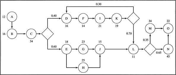
FIGURE 5.15 Flowchart for Exercise 14
TABLE 5.16 Data for Exercise 14

- A reengineering team has studied a process and has developed the flowchart in Figure 5.16. The team also has determined that the expected waiting and processing times (in minutes) corresponding to each activity in the process are as shown in Table 5.17.
- Calculate the average cycle time for this process.
- Calculate the cycle time efficiency.
- A process design team is analyzing the capacity of a process. The team has developed the flowchart in Figure 5.17. The numbers between parentheses indicate the processing times in minutes, and the labels above or below each activity indicate the resource type (i.e, R1 = resource 1). The process has one unit of resource R1, two units of resource R2, and three units of resource R3. Assume that a reworked job has the same chance to pass inspection as a regular job.
TABLE 5.17 Data for Exercise 15

- Calculate the theoretical process capacity and identify the bottleneck.
- If the actual throughput rate of the process is one job per hour, what is the capacity utilization?

FIGURE 5.17 Flowchart for Exercise 16
- Use the theory of constraints and the data in Tables 5.18 and 5.19 to determine how many units of each job type should be completed per week in order to maximize profits. Consider that the availability is 5,500 minutes for resource R1, 3,000 minutes for resource R2, and 8,000 minutes for resource R3.
TABLE 5.18 Routing, Demand, and Profit Data for Exercise 17

TABLE 5.19 Processing Times and Resource Assignments for Exercise 17

- An order-fulfillment process has demand for three order types during the next 4 weeks, as shown in Table 5.20. The assignment of activities to workers and processing time for each activity are shown in Table 5.21. All workers have 40 hours per week available to work on this process. Use the TOC principles to find the number of orders of each type that should be processed to maximize total profit.
TABLE 5.20 Data for Exercise 18

TABLE 5.21 Data for Exercise 18


