CHAPTER 8
Modeling And Simulating Business Process
Chapter 7 introduced the basic elements of Extend and showed how to use them to build a simple queuing model. The model was then expanded to add more than one server and a labor pool. These basic elements can be used to model simple processes, but in some cases they are not sufficient to model realistic business processes consisting of a potentially large set of activities, resource types, and complex job routings and information structures. This chapter explores additional Extend tools with the goal of modeling and simulating business processes found in practice. Recall that the process-flow analysis in Chapter 5 considered that activity times were deterministic (i.e., the times were certain and there was no variation). However, in practical settings, the processing times typically are not deterministic; therefore, process performance must be assessed taking into consideration the variability in the process. In general, three types of variability are relevant in business processes: (1) variation in the arrival of jobs, (2) variation in the processing time of each activity, and (3) variation in the availability of resources. Along with variability, these simulation models will add other realistic elements of business processes that the basic analysis tools of Chapters 4, 5, and 6 cannot easily incorporate.
The best way to learn the material discussed in this chapter is to read it while using Extend and to look at the simulation models found on the CD that accompanies this book. For convenience, all the models used for illustration purposes have been included in the CD. The simulation models in the CD are named Figurexx.xx.mox; xx.xx corresponds to the figure number in the book. For instance, the first model that is discussed in this chapter is the one that appears in Figure 8.2. Its corresponding file is Figure08.02.mox.
8.1 General Modeling Concepts
All simulation models share five general concepts:
- Selection of time units
- Length of a run
- Number of runs
- Model verification
- Model validation
8.1.1 SELECTION OF TIME UNITS
Although Extend allows models to be built with generic time units, it is generally more practical to establish a default time unit. To establish the default time unit in the model, select Run > Simulation Setup… and change the global time units in the Time Units tab. The parameter values also can be selected to convert hours into days and days into years on this tab. Once a global time unit is selected, all time-based parameters in the blocks in the model will be set to the selected time unit. The selected global time unit becomes the default time unit throughout the model. Note that it is possible to use other time units within a block. For example, the global time unit might be set to hours, but a processing time for an activity could be given in minutes. Extend will make the right conversions to establish a single time unit during the simulation run. If the global time units are changed from hours to minutes, all parameters set to the default time units also will change from hours to minutes. The default time unit is marked with an asterisk (*) in the dialogue window of a block.
In some cases, it might not be desirable to leave a parameter set to the default time unit, because a global change in the model could introduce an error. For example, suppose the processing time of an activity is 2 hours. If the global time unit is hours and the processing time is set to the default time unit, the model will be correct as long as the global time unit is not changed. However, if the global time unit is changed to days, then the processing time of the activity will be 2 days instead of 2 hours. To avoid this, use a local time unit for the block and set it to 2 hours (without the asterisk), indicating that the time units will not be affected by changes to the global time unit.
8.1.2 LENGTH OF A RUN AND NUMBER OF RUNS
Another important consideration when building a model is the length of a run and the number of runs. The selection of end time and number of runs in the Discrete Event tab of the Simulation Setup dialogue typically depends on the following four factors.
- Whether the process is terminating (has a natural end point) or nonterminating (has no obvious end point).
- The period of interest (i.e., the portion of time being modeled).
- The modeling objectives (e.g., estimating performance or exploring alternative designs).
- The method in which samples for statistical analysis are obtained (e.g., from running multiple short simulations or analyzing portions of a long one).
Some processes have an obvious termination point. In these terminating processes, there is a point in time when no more useful data will be obtained by running the simulation any longer. Most service processes have a point at which activities end. Setting the end time at 8 hours, for example, can safely simulate a walk-in customer service center that is opened 8 hours per day. Customers will not wait overnight at the queue, so the process is emptied before the beginning of a new day (i.e., the beginning of a new simulation run). Because terminating processes typically do not reach a steady state (see Section 9.5.2), the purpose of the analysis usually is to identify trends and look for changes rather than to obtain long-run statistics, such as average performance. In the customer service center, it would be more relevant to identify peaks and valleys for the activity level than to calculate averages. Basing decisions on average utilization in this case could obscure transient problems caused by multiple periods of understaffing.
Because the initial conditions in terminating processes affect results, it is important for these conditions to be realistic and representative of the actual process. An initial condition for the customer service center example might establish the number of people waiting in line when the doors are opened in the morning. If the actual process starts empty, then no initial conditions need to be set in the simulation model. This might be the case for a movie theater at the beginning of each day. Terminating processes are simulated using multiple runs, whereby each run represents a natural breaking point for the process (e.g., each run might represent a working day). The selection of a given random seed affects the output data obtained from a set of runs. The random seed can be changed in the Random Numbers tab of the Simulation Setup dialogue.
The length of the simulation is usually not an issue when dealing with terminating processes because of their natural end point. For example, the simulation of a bank branch that is open to the customers from 9 A.M. until 4 P.M. could be set to end after 7 hours. However, sometimes a particular period of operation of a terminating process might be of interest; therefore, the starting and ending of the simulation could be adjusted to collect data for this period of interest. In the bank example, a period between 11 A.M. and 2 P.M. might be of interest and therefore simulated a number of times to collect relevant data.
Nonterminating processes do not have a natural or obvious end time. Models of nonterminating processes are often referred to as steady-state processes, because they tend to reach steady state when run for a long period of time. (See Section 9.5.1.) Some service operations such as a 24-hour grocery store, emergency rooms, and special call centers are nonterminating processes. Many business processes are also nonterminating, because the work-in-process remains in the process from one day to the next. For example, an order-fulfillment process that does not complete an order in a given day might finish the processing during the next working day. Hence, business processes that do not “clear out” at the end of a working day can be considered nonterminating. In order to simulate 30 working days of a nonterminating business process, the end time is set to 30*8 = 240 hours, considering 8-hour working days. Thus, a single run of 240 hours of a nonterminating process corresponds to 30 runs of 8 hours of a terminating process. Note that the initial conditions for each day in a nonterminating process depend on the final state of the process at the end of the previous day. On the other hand, the initial conditions at the beginning of each day in a terminating process are typically the same from one run to the next.
One of the important considerations when simulating nonterminating processes is the determination of the warm-up period. This is the period between the beginning of the simulation (when the process is initially empty) and the time when the process operates at a normal or steady-state level. If data are collected during the warm-up period, measures of performance will be biased. A realistic picture of the steady-state performance of a process is obtained when data are collected after the warm-up period. Another way of minimizing the effect of the warm-up period is to run the simulation model for an extended period of time. In this way, the data collected after the warm-up period will “swamp” the bias caused by the initial conditions. To obtain multiple samples for statistical analysis, a nonterminating process can be run several times (with different seeds for the random number generator). As is the case with terminating processes, the greater the number of samples is, the higher the statistical confidence is.
In contrast with terminating processes, determining the length of the run in nonterminating processes can be difficult. Theoretically, a nonterminating process can run indefinitely. In practice, the length of the run is related to the time the process requires to reach steady state. Also, the length of the run should be such that all the events that are possible in a simulation happen at least once. For example, a model might include an event that simulates a machine breaking down; therefore, the length of the run should be such that this event happens at least once so its effects can be analyzed.
8.1.3 MODEL VERIFICATION
Model verification is the process of debugging a model to ensure that every portion operates as expected (i.e., that the model behaves as expected given the logic implemented). One way of verifying that the model is correct is to use an incremental building technique. This means that the model is built in stages and run at each stage to verify that it behaves as expected. Another technique is to reduce the model to a simple case for which the outcome can be easily predicted. This simplification can be obtained as follows.
- Remove all the variability to make the model deterministic.
- Run the deterministic model twice to verify that the same results are obtained.
- For processes with several job types, run the model using one job type at a time.
- Reduce the size of the labor pool (e.g., to one worker).
- Uncouple interacting parts of the model to see how they run on their own.
Other techniques for verification include accounting for all the items in the model and adding animation. After the model is verified, it needs to be validated.
8.1.4 MODEL VALIDATION
Model validation refers to determining whether the model represents the real process accurately. A valid model is a reasonably accurate representation of the real processes that conforms to the model’s intended purpose. During validation, the analyst needs to be sure that comparisons against a real process are made using the same metrics (i.e., that measures of performance are calculated in the same manner). Determining whether the model makes sense is often part of validating a model. The analyst also can ask someone familiar with the process to observe the model in operation and approve its behavior. Simulation results also can be compared with historical data to validate a model. If enough historical data are available (for example, arrival and processing times), these data can be used to simulate the past and validate that the model resembles the actual process under the same conditions.
8.2 Items and Values
Within an Extend simulation model, an item is a process element that is being tracked or used. For example, items being tracked (transient entities) could be jobs, telephone calls, patients, or data packets. Items being used (resident entities) could be workers, fax machines, or computers. Items are individual entities and can have unique properties (for example, a rush order versus a normal order) that are specified by their attributes and priorities. An item can only be in one place at a time within the simulation model. Items flow in a process and change states when events occur. For example, a server could change from idle to busy when a customer arrives.
Values provide information about items and the state of the simulated process. Values can be used to generate output data such as the waiting time in a queue or the actual processing time of an activity. These values will be referred to as output values. Output values include statistics such as the average queue length and the average utilization of a resource. There are also state values, which indicate the state of the process. For example, the number of customers waiting in line at a given time indicates the state of the system. Most blocks in Extend include connectors that can be used to track output or state values.
8.2.1 GENERATING ITEMS
The simulation of a business process typically starts with a job entering the process. Arrivals are generally random, because in most situations that don’t deal with scheduled appointments, it would be difficult (or even impossible) to predict when the next job will arrive. Most of the time, all the analyst can hope for is to be able to assign a pattern (a probability distribution function) to the time elapsed between one arrival and the next. The Import block from the Generators submenu of the BPR library or the Generator block from the Discrete Event library is the most common method used for generating random arrivals in Extend. The focus here will be on how to use the Import block. The dialogue window of this block contains a pop-up menu with several probability distribution choices. Figure 8.1 shows the dialogue of the Import block set to generate one item every 6 minutes (on average) using an exponential distribution; that is, the interarrival times are exponentially distributed with a mean of 6 minutes.
Other probability distributions (uniform, triangular, or normal) can be used to model the interarrival times with an Import block. The selection of a distribution depends on the business process under study and the outcome of a statistical analysis of input data (as described in Chapter 9). In the Import block dialogue, parameters of the chosen distribution are assigned consecutive numbers. For example, the exponential distribution has only one parameter, the mean; therefore, this parameter is labeled number one (l). The normal distribution has two parameters, the mean and the standard deviation, so the mean is parameter number 1 and the standard deviation is parameter number 2. The connectors labeled 1 and 2 at the bottom of the Import block are used to set the values for the distribution parameters from outside of the block.
In addition to specifying the pattern of interarrival times, one can specify the number of items to be generated per arrival by the Import block. (See the # of Items(V) box in Figure 8.1.) The typical item value V is 1, meaning that one item is generated per arrival. However, suppose a process receives jobs in batches of 10 every 2 hours (with no variation). To model this situation with an Import block, change the Distribution to constant, make the constant value equal to 2, and change the time units to hours. In addition, change the # of items (i.e., the V value) to 10. This means that the Import block will generate an item with a V value of 10 every 2 hours. When an item with V = 10 arrives to a resource-type block or a queue, the item is split into 10 individual items with V = 1.

FIGURE 8.1 Import Block Dialogue Showing Exponential Interarrival Times with Mean of 6 Minutes
In some practical settings, the rate of arrivals (or the mean time between arrivals) changes during the simulation. For example, the rate of customers arriving to a dry cleaner is larger in the morning and evening than during the day. Changes can be modeled in the interarrival times with an Input Data block from the Inputs/Outputs submenu of the Generic library. (See Figure 8.2.)
Suppose that in the dialogue of the Import block, the exponential distribution is chosen to model the time between job arrivals. The mean of the distribution is labeled (1) Mean = in the Import block. When the output of the Input Data block is connected to the 1 input connector of the Import block, the mean of the distribution overriding the value in the Import block dialogue is changed. This allows one to dynamically change the average time between arrivals. Suppose that the time between arrivals at a dry cleaner is 30 seconds between 8 A.M. and 9 A.M. and between 5 P.M. and 6 P.M.; the rest of the day it is 5 minutes. If the simulation model is such that each run represents a 10-hour working day from 8 A.M. until 6 P.M., then the Input Data dialogue in Figure 8.3 can be used to model the changes in the mean interarrival time. It is assumed that the Import block uses minutes as the time unit and that the probability distribution is set to exponential.

FIGURE 8.2 Input Data Block Used to Change the First Parameter of the Interarrival Time Distribution in theImport Block

FIGURE 8.3 Input Data Block Dialogue for Dry Cleaner Example
The dialogue in Figure 8.3 shows that the mean interarrival time is half of a minute (or 30 seconds) during the first and last hour of a 10-hour simulation. The mean interarrival time is 5 minutes the rest of the time. Note that the time units in the Import block must be set to minutes, but the time units in the Input Data block are hours. In other words, the time unit of the Time column in the dialogue of Figure 8.3 is hours, and the time unit in the Y Output column is minutes.
Instead of generating arrivals at random times, some models require the generation of arrivals at specific times. This generation of arrivals is referred to as scheduled arrivals. The Program block (see Figure 8.4) from the Generators submenu of the Discrete Event library can be used to schedule item arrivals to occur at given times. For example, suppose that an order-fulfillment process receives 500 orders per week and almost all of the orders are received on Tuesday. Also suppose that the time unit of the simulation is days and that the model is set up to run for 1 week. Then the arrival times are entered in the Output Time column, and the number of orders is entered in the Value column of the Program block, as shown in Figure 8.4.

FIGURE 8.4 Program Block (and Dialogue Window) Connected to a Stack Block for the Order Fulfillment Example
In the Program block, the actual arrival time is entered in the Output Time column instead of the interarrival time, as done in the Import block. The order-fulfillment example has five arrival events (one for each day of the week), and the item values range from 40 to 300. The table in Figure 8.4 indicates that 40 orders are received on Monday, 300 on Tuesday, and so forth. To avoid “losing” items in the simulation, follow a Program block with a Stack block (from the Queues submenu of the BPR library). Like in the case of the Import block, the Program block generates items with values greater than 1 as a batch of items arriving at the same time. When the batched itemgoes to the Stack block, it becomes multiple copies of itself. For example, as each order item is input from the Program block to the Stack block, it will become 40, 300, or 50 orders, depending on the given value.
8.2.2 ASSIGNING ATTRIBUTES TO ITEMS
Attributes play an important role in business process simulations. An attribute is a quality or characteristic of an item that stays with it as it moves through a model. Each attribute consists of a name and a numeric value. The name identifies some characteristic of the item (such as Order Type), and a number specifies the value of the attribute (for example, 2). It is possible to define multiple attributes for any item flowing through the simulation model. The easiest way to set item attributes is to use the Import block (although this also can be done in the Operation, Repository, Labor Pool, and Program blocks). The Discrete Event library also has two separate blocks for assigning attributes: Set Attribute and Set Attribute (5). In the Attribute tab of these blocks, it is possible to either select an attribute from the pop-up menu or create a new attribute. After an attribute has been selected or a new one has been created, the value of the attribute is entered in the box labeled Attr. Value =. Extend also provides a way of dynamically changing the values of up to three attributes using the Operation block. However, the dynamic modification of attributes is beyond the scope of this book.
Attributes are commonly used to specify the amount of processing time required, routing instructions, or item types. For example, an Operation block could use attribute values to determine the amount of operation time needed for an item. Attributes are used to specify things like “item needs final check” or “send item unchecked.” In this case, depending on the value of the attribute, the item is sent to an Operation block for the final check or the activity is skipped. The use of attributes will be illustrated in the context of routing in Section 8.4. In the Discrete Event library, the Get Attribute block reads the value of a given attribute for every job passing through it. The attribute value is then made available through one of the value connectors of this block. This can be useful in modeling business processes with complex logic and information structures.
8.2.3 PRIORITIZING ITEMS
Priorities are used to specify the importance of an item. When comparing two priority values, Extend assigns top priority to the smallest value (including negative values). Priorities can be set in different ways within an Extend model; however, if the Import block is used to generate arrivals, the easiest is to set the item’s priority in the Attributes tab. Also, the Set Priority block in the Discrete Event library assigns priorities to items passing through it. Priorities are useful when the processing of jobs does not have to follow a first-in-first-out discipline. For example, priorities can be used to model a situation in which a worker examines the pending jobs and chooses the most urgent one to be processed next. In Extend, items can have only one priority.
The Stack block in the Queues submenu of the BPR library allows the order in which items will be released from the queue to be set. The default order is first-in-first-out. Choosing Priority from the pop-up menu of the Queue tab causes the Stack block to choose the next item based on priority value. (See Figure 8.5.)

For an item to be ranked by priority, other items must be in the group at the same time. In other words, items will be sorted by their priority value in a Stack block only if they have to wait there with other items.
8.3 Queuing
Reducing non-value-added time is one of the most important goals in process design. Quantifying the amount of unplanned delays (such as waiting time) is critical when designing new processes or redesigning existing processes. Statistics such as average and maximum waiting time represent useful information for making decisions with respect to changes in a process under study. In order to collect waiting time and queue length data, queues need to be added to the simulation model. The Stack block in the Queues submenu of the BPR library provides different types of queues or waiting lines.
The Stack block has several predefined queuing disciplines, as shown in Figure 8.5. The FIFO option models a first-in-first-out or first-come-first-served queue. The LIFO option models a last-in-first-out queue. The Priority option checks the items’ priorities and picks the item with the highest priority (the smallest priority value) to be released first. If all the items in the queue have the same priority, then a FIFO discipline is used. The Reneging option can be used to specify how long an item will wait before it reneges, or prematurely leaves. An item will wait in the queue in a FIFO order until its renege time (the maximum amount of time the item is allowed to spend in the queue) has elapsed. At that point, it will exit through the lower (renege) output connector.
8.3.1 BLOCKING
Queues are used to avoid blocking. Blocking occurs when an item is finished processing but is prevented from leaving the block because the next activity is not ready to pick it up (or the next resource block is full). Blocking can occur in serial processes where activities are preceded by queues. For example, consider two activities in a serial process, where activity B follows activity A. Suppose this process has two workers, one who performs activity A and one who performs activity B, and the workers don’t have an In Box, or queue. If activity A is completed while activity B is still in process, the worker performing activity A is blocked, because that person cannot pass on the item until the other worker completes activity B. Adding a queue to activity B eliminates the blocking problems because completed items go from activity A to the queue from which the worker performing activity B picks them.
8.3.2 BALKING
In service operations, customers sometimes enter a facility, look at the long line, and immediately leave. As discussed in Chapter 6, this is called balking. A Decision(2) block from the Routing submenu of the BPR library can be used to model balking. Figure 8.6 shows a process with one queue and balking. Customers are generated at the Import block with an exponentially distributed interarrival time (mean = 1 minute) and go to the Decision(2) block to check on the length of the queue. The length of the queue is passed from the L connector of the Stack block to the Decisio1n(2) block. The current length is used to decide whether the customer will leave or stay. In Figure 8.6, if the length of the queue is five or more, the customer leaves. If the customer leaves, he or she goes to the Export block. If the customer stays, he or she joins the queue (that is, the Stack block) and eventually is served in the Operation block, which has a constant processing time of 1.5 minutes.
The model in Figure 8.6 has two Export blocks to keep track of the number of customers served versus the number of balking customers. The Decision(2) block employs the logic shown in Figure 8.7, which sends customers to the YesPath if QLength is greater than or equal to 5.
In this case, Qlength is the variable name given to the input of the first connector at the bottom of the Decision(2) block. The names Path, YesPath, and NoPath are system variables from Extend.
8.3.3 RENEGING
Another important queuing phenomenon is reneging. Reneging occurs when an item that is already in the queue leaves before it is released for processing. An example of reneging is a caller hanging up before being helped after being put on hold. Figure 8.8 shows a model that simulates this situation. Suppose the customer hangs up if the waiting time reaches 5 minutes. The Import block in Figure 8.8 generates calls with interarrival times exponentially distributed with a mean of 3 minutes. It is assumed that the processing time of a call is uniformly distributed between 2 minutes and 5 minutes. (The duration of the call is modeled with an Input Random Number block from the Inputs/Outputs submenu of the Generic library.)

FIGURE 8.6 Model of a Single Server with a Queue, Where Customers Balk if the Line Reaches a Specified Number of Customers

FIGURE 8.7 Dialogue Window of the Decision(2) Block of Figure 8.6
In the model in Figure 8.8, the Stack block (labeled Calls on Hold) is of the reneging type. To set the stack type, Reneging was chosen in the Type of Stack pop-up menu in the Queue tab of the Stack block. The Renege Time is set to 5 minutes, as shown in Figure 8.9.

FIGURE 8.8 Model of a Single Server with a Queue, Where Customers Hang Up After Being on Hold for a Specified Amount of Time

In this example, a call waits on hold until one of the two representatives is available to answer the call. The Transaction block (labeled Helping Customers) from the Activities submenu of the BPR library is used to model the two customer service representatives. The maximum number of transactions in the Activity tab of the Transaction block is set to 2. The Stack block uses the waiting time of the calls on hold to decide whether to release a call to the Transaction block through the upper output connector or to the Export block through the lower output connector.
The renege time can be adjusted dynamically using the R input connector of the Stack block. Although this model uses an Export block to count the number of lost calls, this is not necessary because the Stack block keeps track of the number of reneges and displays it in the Results tab. Because items that renege leave the Stack block through the output connector on the lower right, these items can be rerouted back to the original line or to other activities in the process.
8.3.4 PRIORITY QUEUES
As discussed in Section 8.2.3, when a block downstream can accept an item, a priority queue searches through its contents and releases the item with the highest priority (i.e., the item with the smallest priority value). The Stack block can be set to operate as a priority queue by selecting Priority in the Type of Stack pop-up menu.
Consider the following situation. Patients arrive at a hospital admissions counter, and 20 percent of the time they cannot be admitted because they need to fill out additional forms. After they fill out additional forms, they come back to the counter to complete the admissions process. Patients returning to the counter are given higher priority and can go to the front of the line. To model this situation, generate arriving patients and set their priority to 2. This is done in the Import block from the Generators submenu of the BPR library. In the Attributes tab of the Import block, the priority of the items being generated can be set to a value of 2. In this way, priority 1 can be used for patients who return to the line after filling out the additional forms. Figure 8.10 shows a simulation model of this simple admissions process.

FIGURE 8.10 Admissions Process with a Priority Queue That Allows Patients to Go in Front of the Line After Filling Out Additional Forms
The model in Figure 8.10 shows that a Select DE Output block from the Routing submenu of the Discrete Event library is used to simulate the percentage of patients needing to fill out the additional forms. In the Select Output tab of the dialogue window of the Select DE Output block, the Do Not Use Select Connector box should be checked. Also, Route Items by Probability should be selected, and a probability value of 0.2 should be used for the top output. The dialogue window of the Select DE Output block is the same as the one shown in Figure 7.23.
It is assumed that the clerk gives the forms to the patients, and after a constant time (simulated with the Transaction block labeled Filling Out Additional Forms), the priority of the patients is changed and they are sent back to the queue. The dialogue of the Stack block that models the priority queue is shown in Figure 8.11.

FIGURE 8.11 Dialogue Window of the Stack Block in Figure 8.10
The Set Priority block from the Attributes submenu of the Discrete Event library is used to change the priority of the patients from 2 to 1. After the priority is changed, patients who return to the queue have higher priority than patients who just arrived. As mentioned earlier, Extend uses a FIFO queue discipline when all the items in a queue have identical priority values.
8.4 Routing
When modeling business processes, it is common to encounter situations where jobs come from different sources or follow different paths. For example, Figure 8.10 shows that the clerk’s line receives newly arriving patients and patients who completed additional paper work. In other words, the Stack block that simulates the queue receives patients from two different sources: the Import block that simulates the patients arriving to the hospital, and the Transaction block simulating the patients filling out additional forms. The patients coming from these two sources are merged into one stream with the Merge block; however, the patients remain as individual items and retain their unique identity.
The Merge block in the Routing submenu of the BPR library can merge items from up to three separate sources. Another example of merging items from different sources occurs when telephone orders and mail orders are directed to an order-entry department. Also, the Merge block can be used to simulate workers returning to a labor pool from different parts of a process. (Resources and labor pools are discussed in Section 8.7.)
Chapter 5 introduced two types of routing: multiple paths and parallel activities. This chapter will now discuss how to simulate these routing conditions with Extend.
8.4.1 MULTIPLE PATHS
Jobs do not usually arrive, join a queue, get completed in a single step, and leave. If this were true, every process could be simulated with an Import block (to generate arrivals), a Stack block (to simulate a queue), an Operation block (for the service activity), and an Export block (for jobs leaving after the completion of a single activity). Real-world business processes call for routing jobs for processing, checking, approval, and numerous other activities. The simulation models must be capable of routing jobs based on a probability value, logical and tactical decisions, or job characteristics.
Probabilistic routing occurs when a job follows a path a specified percentage of the time. For example, Figure 8.10 shows a model in which 20 percent of the time hospital patients cannot be admitted because they need to fill out an additional form. A rework loop shares this characteristic. That is, after an inspection (or control) activity, jobs are sent back for rework with a specified probability. In Figure 8.10, a Select DE Output block from the Routing submenu of the Discrete Event library was used to model a probabilistic routing with two paths. To model probabilistic routing with up to five possible paths, a Decision(5) block and a Random Input block are needed. Suppose a job follows one of three possible paths (labeled 1, 2, and 3) with probabilities 0.2, 0.3, and 0.5, as shown in Figure 8.12.
This situation is simulated by first generating jobs with an Import block and then adding a Decision(5) block to probabilistically route each job, as illustrated in Figure 8.13.
In the Input Random Number block, an Empirical table is chosen from the Distribution pop-up menu. The values in the Empirical table reflect the probability that a job follows each path, as shown in Table 8.1. Therefore, the path number is probabilistically determined in the Input Random Number block and is sent to the first connector of the Decision(5) block.


FIGURE 8.13 An Illustration of Probabilistic Routing with Extend
The Decision(5) block is set to read the path number from the Input Random Number block and use this number to route the current job to one of the three paths. The name of the first connector is specified as PathNum, and the value is used in the routing logic box to force the selection of each path according to the given path number.
if (PathNum == 1) Path = Pathl;
if (PathNum == 2) Path = Path2;
if (PathNum == 3) Path = Path3;
Although the default path names Pathl, Path2, and Path3 are used in this example, the Decision(5) block allows the path names to be changed to ones that are more descriptive in terms of the process being modeled. Also, the paths in this example simply consist of an Export block that counts the number of jobs routed in each direction. In a real process, the paths would consist of multiple activities and possibly even a merging point later in the process.
In addition to probabilistic routing, business process models often include tactical routing. This type of routing relates to the selection of paths based on a decision that typically depends on the state of the system. For example, suppose one wants to model the checkout lines at a supermarket where customers choose to join the shortest line. Figure 8.14 shows an Extend model of this tactical decision.
TABLE 8.1 Empirical Probability Table in Input Random Number Block

The Import block in Figure 8.14 generates the customers arriving to the cashiers. Each cashier is modeled with an Operation block and the independent lines with Stack blocks. The model connects the L (queue length) connector from each Stack block to a Max & Min block from the Math submenu of the Generic library. This block calculates the maximum and the minimum of up to five inputs. The Max and the Min output connectors give the maximum and the minimum values, respectively. The Con connector tells which of the inputs generated the largest or the smallest value. The equation in the Decision(5) block dialogue decides the routing based on the value provided by the Max & Min block:
if(MinQ == 1) Path = Line1;
if(MinQ == 2) Path = Line2;
if(MinQ == 3) Path = Line3;

FIGURE 8.14 Illustration of Tactical Routing with Customers Choosing the Shortest Line
MinQ is the name assigned to the first input connector in the Decision(5) block. The Line1, Line2, and Line3 names are the labels used for each path. If the lines have the same number of customers, the incoming customer joins the first line. This is why even when the cashiers work at the same speed, the first cashier ends up serving more customers than the other two. (See the Export blocks in Figure 8.14.) This could be corrected with additional logic that randomly assigns a customer to a queue when all queues have the same length.
8.4.2 PARALLEL PATHS
Some business processes are designed in such a way that two or more activities are performed in parallel. For example, in an order-fulfillment process, the activities associated with preparing an invoice can be performed while the order is being assembled, as depicted in Figure 8.15.
In Figure 8.15, the order is not shipped until the invoice is ready and the order has been assembled. To model parallel paths with Extend, use the Operation, Reverse block in the Batching submenu of the BPR library. This block separates an incoming item into multiple copies and outputs them one at a time. For each output connector (up to a total of three), the number of copies to be created can be specified. Figure 8.16 shows the Operation, Reverse block along with its dialogue.
The dialogue in Figure 8.16 shows that the Operation, Reverse block is set to create two copies of the input item. One copy will be sent through the top output connector, and the other copy will be sent through the bottom connector. After the activities in each parallel path are completed, an Operations block from the Activities submenu of the BPR library is used to batch the corresponding items into one. This block batches items from up to three inputs into a single item. In the dialogue of this block, it is possible to specify the number of items required from each input to create a single output item. All required inputs must be available before the output item is released. Figure .8.17 shows the dialogue for the Operation block.
Each input connector that is used must have a quantity of items strictly greater than zero specified in the dialogue. Figure 8.17 shows that an item from the top input connector and an item from the bottom input connector are needed to create a single output item.
Figure 8.18 shows the “skeleton” (without timing information) of an Extend model for the order-fulfillment process depicted in Figure 8.15. Orders are generated with the Import block and are sent to the Operation block labeled Receiving Order. The Operation, Reverse block creates two copies of the order and sends one to Prepare Invoice and another one to Assemble Order. After both of these activities are completed, the activity Shipping Order is performed.

FIGURE 8.15 Parallel Activities in on Order-Fulfillment Process


FIGURE 8.17 Operation Block That Batches Two Items
Parallel paths can consist of more than one activity each. In the model in Figure 8.18, each parallel path consists of one activity, but the same modeling principles applied to paths with multiple activities. That is, an Operation, Reverse block is needed to create copies of the job, and then an Operation block is needed to transform the multiple copies into one.

FIGURE 8.18 Extend Model of the Order-Fulfillment Proces in Figure 8.15
8.5 Processing Time
One of the key tasks when creating simulations of business processes is modeling the processing time of activities. In Extend, the Operation block or the Transaction block is used to model activities. The main difference between these two blocks is that the Operation block can process only one item at a time, and the Transaction block can process several items at a time (up to a specified limit). Section 7.5 showed how the Transaction block can be used to model processes where multiple servers perform the same activity.
Activities, such as those modeled with the Operation and Transaction blocks, involve a processing time or delay that represents the amount of time it takes to perform the specified task. The Decision(2) and the Decision(5) blocks also include a processing time that is used to model the time to make a decision. Processing time can be static or vary dynamically depending on model conditions. The time can be random, scheduled based on the time of the day, depend on the item being processed, or be affected by any combination of these factors.
The easiest way of setting the processing time is to choose a value in the dialogue of the corresponding block. This, however, is useful only when the processing time is known and does not change throughout the simulation. In other words, it is useful when the processing time is deterministic and constant. For example, if the task of typing an invoice always takes 5 minutes, the value 5 is entered as the processing time in the dialogue of the activity block. On the other hand, if the processing time is not deterministic and constant, the D connector of activity or decision blocks is used to dynamically change the processing time (as shown in Section 7.4).
When the processing time is fixed (i.e., deterministic and constant) but one wants to have the ability to change it from run to run without having to open the corresponding dialogue, a Slider can be added to the model. A Slider, shown in Figure 8.19, is a control that makes simulation models more user friendly.
To add a Slider, select it from Model > Controls. Then click on the maximum and minimum values to change them appropriately. By default, these values are set to zero and one. Next, the middle output connector is connected to the D connector of an activity or decision block. The processing time can now be set by moving the Slider to the desired level. The Slider in Figure 8.19 sets the processing time for the Operation block at 17 time units.
In some situations, the processing time depends on the time of the day. For example, a worker might take longer to perform a task at the end of the day. The Input Data block from the Inputs/Outputs submenu of the Generic library can be used to model this situation. The Input Data block is connected to the D connector of an activity block (e.g., a Transaction block) as illustrated in Figure 8.20, which also shows the dialogue of the Input Data block.

The dialogue in Figure 8.20 shows that the activity is performed in 10 minutes during the first 6 hours of operation and in 12 minutes during the second 6 hours. Note that the time in the Y Output column is given in minutes (because the processing time in the Transaction block is set to minutes), but the values in the Time column are given in hours (which is the time unit used as the default for the entire simulation model).

FIGURE 8.20 Input Data Block to Model Variable Processing Time

One of the most common ways of modeling processing times is using a probability distribution. Random processing times that follow a known or empirical probability distribution can be simulated with an Input Random Number block from the Inputs/Outputs submenu of the Generic library (as illustrated in Section 7.4). The output of this block is simply connected to the D connector of the activity block, and the processing time is drawn from the specified probability distribution function.
Finally, an attribute can be used to assign the processing time for a job. Section 8.2.2 discussed how to assign attributes to items. An Import block can be used to assign an attribute to an item in such a way that the attribute value represents the processing time. The attribute name is then identified in the dialogue of the activity block, as shown in Figure 8.21.
In the dialogue of Figure 8.21, it is assumed that the processing time was stored in the attribute named ProcTime when the item was generated with the Import block.
8.6 Batching
In many business processes, paperwork and people coming from different sources are temporarily or permanently batched. For example, memos, invoices, and requestsmight originate from several parts of the process. The batched items move through the process together. For instance, in an office that handles real estate acquisitions, the requests, bids, and real estate analysis come together in an early step and travel as a single item through the rest of the process.
Batching allows multiple items from several sources to be joined as one for simulation purposes. In Section 8.4.2, the Operation block was used to batch items belonging to the same job that were previously split to be processed in parallel paths. Another way of modeling batching with Extend is with the Batch block from the Batching submenu of the Discrete Event library. The Batch block accumulates items from each source to a specified level and then releases a single item that represents the batch. Figure 8.22 shows the Batch block and its dialogue window.

In Figure 8.22, the single item is not produced as the output of the Batch block until an item from the top input connector (a) and an item from the bottom input connector (b) are both available.
Batching is used to accomplish two slightly different tasks: kitting and binding. Kitting occurs when a specified number of items are physically put together and then released as a single item. This is most common when simulating the assembly of different kinds of paperwork into a single package. The batched item may or may not be unbatched at some later point in the process. Typically, the batched item remains that way through the rest of the process. For example, a kit can be formed of an original order, a sales person’s memo, and a release form from the warehouse. This kit is then stored as a single item after the order is shipped.
Binding items is used to reflect situations where one item is required to be associated temporarily with one or more items to flow together through a portion of the process. Items that are batched for this purpose are typically separated from each other later in the simulation. This type of batching or binding is common when simulating labor movement, as shown in Section 7.6. For example, in a customer service process, the customer is coupled with a customer service representative and possibly some paperwork. These items are batched until the service is completed, at which point the customer, the customer service representative, and the paperwork are unbatched so they can follow different paths for the remainder of the process.
When batching workers with paperwork (such as a request or an order), the Preserve Uniqueness box in the Batch block should be checked so that the worker and the paperwork preserve their identity after the unbatching. Suppose a purchasing agent is merged with a purchase order. The purchase order comes into a Batch block as the top input and the purchasing agent comes in as the middle input. Figure 8.23 shows the dialogue of the Batch block with the Preserve Uniqueness box checked. The discussion of a labor pool will be extended in Section 8.7.

When a worker is batched with another item, such as a request or an order, the binding is temporary and the items are unbatched at some point in the process. The unbatching allows the worker to return to a labor pool and the paperwork to continue the appropriate routing through the rest of the process. The Unbatch block in the Routing submenu of the Discrete Event library is used for unbatching items. When dealing with binding, it is important to unbatch items using the same output connectors used when the items were batched in the Batch block. If this is not done, items could be routed the wrong way. For example, the job could get sent to the labor pool and the worker to the remaining processing steps. Figure 8.24 illustrates how to batch and unbatch correctly. In this figure, a nurse is batched with a patient through the c connector of a Batch block and later unbatched and sent back to the labor pool through the c connector of the Unbatch block. The number of items that the Unbatch block outputs should be the same as the number of items batched with a Batch block. The Output boxes in the Unbatch block are used to specify the number of items routed through each output connector for every item that enters the block, as shown in Figure 8.25.
In Figure 8.25, it is assumed that the Unbatch block is being used to separate items that are required to preserve their own identity, such as a worker and a document. As discussed in Section 8.4.2, unbatching also can be used to duplicate an item into several clones of itself. We saw that this can be done with the Operation, Reverse block even if the item has not been batched previously; for example, an order that is received is entered into a computer and printed in triplicate. The printout can be unbatched to represent a packing slip, an invoice, and a shipping copy.
8.7 Resources
Most business processes require resources to perform activities. For example, a customer service representative is the resource used to perform the activities associated with assisting customers. In other words, resources are the entities that provide service to the items that enter a simulation model. In Extend, resources can be modeled explicitly using a resource block or implicitly using an activity block. Activity blocks can represent the resource and the activity the resource is performing. For example, in Figure 7.5, an Operation block was used to represent the team and the underwriting activity. Later a labor pool was used as a source of underwriting teams for the model. (See Figure 7.22.)


FIGURE 8.25 Unbatching Items with an Unbatch Block
The explicit modeling of resources provides the flexibility of tying up resources for several activities. For example, suppose a nurse must accompany a patient through several activities in a hospital admissions process. The model can include a Labor Pool block to simulate the availability of nurses. When a nurse leaves the Labor Pool block and is batched with a patient, the nurse returns to the labor pool only after performing all the activities as required by the process. Figure 8.24 shows a simple Extend model that simulates the arrival of patients and a single operation (triage) that requires a nurse. Patients wait in a waiting area (modeled with the Stack block) until the next nurse is available. After the activity is completed, the nurse returns to the Labor Pool block and the patient exits this part of the process through the Export block.
The Discrete Event library of Extend provides an alternative way of modeling resources with three blocks: Resource Pool, Queue Resource Pool, and Release Resource Pool. Although this alternative way has advantages in some situations over the batching procedure explained previously, the modeling of resources with these blocks is beyond the scope of this book.
8.8 Activity-Based Costing
Many companies use activity-based costing (ABC) as the foundation for business process redesign. The ABC concept is that every enterprise consists of resources, activities, and cost objects. Activities are defined by decomposing each business process into individual tasks. Then the cost of all resources consumed by each activity and the cost of all activities consumed by each product or cost object are tracked (Nyamekye, 2000).
Activity-based costing is a method for identifying and tracking the operational costs directly associated with processing jobs. Typically, this approach focuses on some unit of output such as a completed order or service in an attempt to determine its total cost as precisely as possible. The total cost is based on fixed and variable costs of the inputs necessary to produce the specified output. ABC is used to identify, quantify, and analyze the various cost drivers (such as labor, materials, administrative overhead, and rework) and determine which ones are candidates for reduction.
When a simulation modeled is built, the outputs as well as the resources needed to create such outputs are fully identified. Adding ABC to the model entails entering the costing information into the appropriate block dialogues. Blocks that generate items (e.g., the Import block) or resources (e.g., the Labor Pool block) and blocks that process items (e.g., the Operation and Transaction blocks) have tabs in their dialogues for specifying cost data. These tabs allow one to enter variable cost per unit of time and fixed cost per item or use. Figure 8.26 shows the Cost tab of the Import block dialogue.

FIGURE 8.26 Cost Tab of the Import Block
After the cost information has been entered, Extend keeps track of the cost automatically as the items enter the process, flow through the activities in their routing, and exit. When considering ABC in a simulation model, every item is categorized as either a cost accumulator or a resource. Cost accumulators are the items (or jobs) being processed. Jobs accumulate cost as they wait, get processed, or use resources. For example, suppose one wants to determine the cost of receiving crates at a warehouse. As each shipment arrives, a labor resource is required to unpack crates and stock the contents on the appropriate shelves. In this case, crates are being processed; therefore, they become the cost accumulators. A crate accumulates cost while waiting and while being processed. For example, it might take an employee approximately 30 minutes to unpack a crate. Figure 8.27 shows a model where processing time and the hourly wage are used to calculate the cost of this process.
The calculated cost is then added to the accumulated cost for each crate. More cost is added to the accumulated total as a crate flows through the receiving process. In this case, the crates are generated with an Import block and their cost information is established in the Cost tab of this block. Resources do not accumulate cost, but their cost information is used to calculate the cost that is added to the total of the cost accumulator. For example, suppose the hourly wage of the employees unpacking crates is $9.75. When an employee is batched with a crate, the hourly rate along with the processing time (the time required to unpack the crate) is used to add cost to the total associated with the crate. If a given crate requires 25 minutes to be unpacked, the accumulated cost of the crate is increased by $9.75 × (25/60) = $4.06.
As mentioned previously, Extend has two types of costs: the fixed cost (cost per use or per item) and the variable cost (the cost per unit of time). Cost accumulators have their own fixed and variable costs. The Cost tab in Figure 8.26 shows that the variable cost of a crate is $0.15 per hour. This is the rate charge per hour of waiting. Also, a $3.59 docking fee is charged per crate. This is a fixed cost that is charged per item (i.e., per crate) entering the process.
The Cost tab of resource-type blocks (such as a Labor Pool block) allows the cost per unit of time (e.g., an hourly rate) and the cost per use of the resource (i.e., the fixed cost) to be specified. The cost per time unit is used to calculate and assign a time-base cost to the cost accumulator during the time it uses the resource. The cost per use, on the other hand, is a one-time cost assigned to the cost accumulator for the use of the resource (a fixed service charge). When using a labor pool to model resources and adding ABC, be sure that the Release Cost Resources option is selected in the Unbatch block. This option is at the bottom of the Unbatch tab. Because the cost accumulators and the resources are batched, the unbatching operation needs to release the resources and modify the accumulation of cost before the items can continue with further processing.

FIGURE 8.27 Model to Accumulate Cost per Unpacked Crate
Cost information also can be defined for activities. For instance, within the Cost tab of activity-type blocks (such as an Operation block or a Transaction block), variable and fixed costs can be defined. These cost drivers allow resources to be modeled implicitly (i.e., without a labor pool and the batching method) as done in Figures 7.14 and 7.20.
Cost data are accumulated in two blocks: the Cost by Item block and the Cost Stats block, both from the Statistics submenu of the Discrete Event library. These blocks were introduced in Section 7.3 and used in Section 7.8. Basically, the Cost by Item block collects cost data of items passing through the block. The block must be placed in the model in such a way that the items of interest pass through it at a time when the accumulated cost has the value one wants to track. The Cost Stats collects data for all costing blocks such as an Operation or a Labor Pool block. Figure 8.27 shows the process of receiving and unpacking crates with a Cost Collection block for the crates. The Cost by Item block is placed immediately after the completion of the unpacking activity. Figure 8.28 shows the dialogue of the Cost by Item block after a 40-hour simulation. A total of 79 crates were unpacked during the 40 hours, and the Cost by Item block indicates that the average cost of unpacking a crate is $9.38.

FIGURE 8.28 Dialogue of the Cost by Item Block of the Simulation Model in Figure 8.27
8.9 Cycle Time Analysis
One of the most important measures of process performance is cycle time. In addition to total cycle time (i.e., the time required by an item to go from the beginning to the end of the process), in some cases it might be desirable to calculate the time needed to go from one part of the process to another. In other words, it might be of value to know the cycle time of some process segments in addition to knowing the cycle time for the entire process. In both cases, Extend provides a way of adding cycle time analysis to a simulation model.
The Timer block in the Information submenu of the Discrete Event library is used to calculate the cycle time of individual items. The block is placed at the point where the timing should start. The items enter the block through the input connector. The output connector should send the items out to the rest of the activities in the model. The sensor input is connected to the output of a block that is the ending point for the process or process segment for which the cycle time is being calculated. Figure 8.29 shows a process with two operations and a Timer block before the first operation.
The model has two Stack blocks, where items wait to be processed. The cycle time is measured from the time items arrive and join the first queue to the time the items leave after completing the second operation. The D connector in the Timer block is used to read the individual cycle time values for each item. The Histogram block in the Plotter library is used to create a histogram of the cycle time values for all items. The M connector is used to plot the average cycle time versus the simulation time. This is done using the Plotter Discrete Event block in the Plotter library. Both of these plotters are shown connected to the Timer block in Figure 8.29, and the resulting plots after a 10-hour simulation run are shown in Figure 8.30.
The plots in Figure 8.30 show that the average cycle time seems to be converging to a value between 4.5 and 5 minutes. This needs to be verified through a longer simulation run so that the effects of the warm-up period of the first 150 simulation minutes are minimized. The histogram shows that most of the jobs were completed in 4.3 minutes or less.

FIGURE 8.29 Two Operations in Series with a Timer Block to Measure Cycle Time

8.10 Model Documentation and Enhancements
Section 7.7 discussed the use of simple animation within Extend. Other forms of documenting and enhancing a model are adding text, using named connections, adding controls such as a slider or a meter, and displaying results. Text can be added with the Text tool. Also, the Text menu allows the size and font to be modified, and the Color tool allows the text color to be changed. Named connections are helpful because as the model grows, more connecting lines might intersect and make the model less readable. Named connections were introduced in the model in Figure 7.22. The idea is simple: A text box is created with the name of the connection, and then the box is duplicated (Edit > Duplicate) and an output connector is connected to one copy of the text box and the corresponding input connector is connected to the other copy of the text box.
Extend has three special blocks that can be used to add interactive control directly to the model. These blocks can be chosen with the Controls command in the Model menu. These blocks are used to add interactive control directly to the model. They are used to control other blocks and show values during the execution of the simulation. The controls are Slider, Switch, and Meter. A Slider resembles those typical of stereo systems. A Slider is used in Figure 8.19 to set the processing time of an operation. The maximum and minimum are set by selecting the numbers at the top and the bottom of the Slider and typing the desired values. The output of the Slider can be changed by dragging the level indicator up or down. Figure 8.31 shows the Slider connected to an Input Random Number block that is set to generate a random number from an exponential distribution. The Slider is used to change the mean (parameter 1) of the exponential distribution modeled with the Input Random Number block.
The maximum and minimum values also can be output by connecting their corresponding output connector. The middle connector outputs the current level indicated in the Slider’s arrow.

The Switch control has two inputs and one output and looks like a standard light switch. This control typically is used in connection with blocks that have true-false inputs. The use of this control is beyond the scope of this book, but a detailed description can be found in the Extend user’s manual.
The Meter can be used to show values that vary between a specified maximum and minimum. The maximum and minimum values are set through the Meter’s dialogue or through the top and bottom connectors. The Meter is useful when one wants to monitor a particular value with known maximum and minimum (e.g., the utilization of a certain resource) and there is no interest in saving these values using a plotter block. Figure 8.32 shows a Meter connected to the utilization output of a Labor Pool block.
This chapter has shown how to use the connectors from blocks such as the Timer and the Stack to display results graphically. The results connectors associated with these blocks are connected to plotters such as the Histogram and the Plotter Discrete Event to create graphical displays during the simulation. Another easy way of displaying results during the execution of the simulation is by cloning. Suppose one wants to display the average waiting time in a Stack block as it is updated during the simulation. Open the dialogue of the Stack block and click on the Results tab. Then click on the Clone Layer tool (see Figure 8.33), highlight the Average Wait text and value box, and drag them to the place in the model where they are to be displayed.
The Clone Layer tool creates a copy of the chosen items and allows them to be placed in the model to enhance documentation and animation.
Chapter 7 and the first 10 sections of this chapter have introduced Extend blocks and functionality that are relevant to building simulation models of business processes. This chapter concludes with two process design cases that make use of many of the concepts that have been discussed so far.

FIGURE 8.32 Meter Connected to the Utilization Output of Labor Pool Block

8.11 Process Design Case: Software Support
This section shows how a simulation model can be used to analyze and improve the efficiency of a relatively simple business process. The setting for this process is a call center that handles requests for software support1.
The manager of a software support organization that provides phone and e-mail help to users wants to use simulation to explain why the productivity of the group is less than he thinks it should be. His goal is to redesign the support processes so that time to completion for problem resolution is reduced. The facilitator working with the manager would like to use this goal to define parameters by which the process can be measured. The facilitator knows that establishing a goal early in a modeling effort will allow her to determine the attributes of the process that will have to be investigated. In addition, this also will help in the task of interviewing process participants.
Before interviewing the process participants, the facilitator asked for any documentation about the process that was available. The documentation of the process and the flowcharts treat phone and e-mail support as separate processes. (See Figure 8.34.) However, the reality is that in addition to reviewing and solving problems that have been submitted in writing, support personnel also have to answer phone calls. In fact, answering the telephone, or real-time response, was given priority over providing e-mail help. The support personnel have suggested to management that one person should handle all the phone calls, and the others should handle problems submitted via e-mail. The request has been ignored, because management has concluded that: (1) There is time to perform both activities, and (2) with three support personnel, if one only takes phone calls, a 33 percent reduction in problem-solving productivity will result.
In an effort to better understand the interaction between the e-mail software support system and the phone call process, the facilitator has collected data and made the following assumptions.
- Requests for software support arrive at a rate of about 18 per hour (with interarrival times governed by an exponential distribution). Two-thirds of the requests are e-mails and one-third are phone calls.
- E-mails require an average of 12 minutes each to resolve. It can be assumed that the actual time varies according to a normal distribution with mean of 12 minutes and standard deviation of 2 minutes.

FIGURE 8.34 Documented Software Support Process
- The majority of the phone calls require only 8 minutes to resolve. Specifically, it can be assumed that the time to serve a phone call follows a discrete probability distribution where 50 percent of the calls require 8 minutes, 20 percent require 12 minutes, 20 percent require 17 minutes, and 10 percent require 20 minutes.
Given this information, the manager of the group has concluded that he is correct in his assumption that with a little extra effort, support personnel can handle e-mails as well as phone calls. His logic is the following: 96 e-mails (12 e-mails/hour × 8 hours) at 12 minutes each require 1,152 minutes, and 48 phone calls (6 calls/hour × 8 hours) at an average of 8 minutes each require 384 minutes. That totals 1,536 minutes, or 3 working days of 8 hours and 32 minutes. He reasons that his personnel are professionals and will work the required extra 32 minutes.
8.11.1 MODELING, ANALYSIS, AND RECOMMENDATIONS
First, one should take a closer look at the manager’s reasoning. The manager has based his calculations on the assumption that it takes an average of 8 minutes to resolve problems reported by phone. Although half (50 percent) of the calls require 8 minutes, the average call requires 11.8 minutes (8 × 0.5 + 12 × 0.2 + 17 × 0.2 + 20 × 0.1). Furthermore, the probability is fairly large (30 percent) that a phone call will require 17 or more minutes, which more than doubles what the manager is using for his calculations. He also is ignoring the variability of the arrivals of requests for technical support.
The manager is concerned with the group’s productivity, which he most likely defines as the ratio of resolved problems to total requests. In addition to this, he would like to reduce the time needed to resolve software problems. Controlling the time to resolve a problem might be difficult, so the reduction in cycle time must come from reductions in waiting time. This is particularly important when handling phone calls because customers are generally irritated when they have to spend a long time on hold.
The process currently in use can be analyzed by modeling the work of one of the support people. To do this, adjust the arrival rates of e-mails and phone calls to represent what a single support person observes. According to the aforementioned arrival rates, the interarrival times are 5 and 10 minutes for e-mails and phone calls, respectively. If three support people are working, each of them experiences interarrival times of 15 and 30 minutes for e-mails and phone calls, respectively.
Figure 8.35 shows a simulation of one support person in the actual process. Two Import blocks are used to model the arrivals of e-mails and phone calls separately. E-mails are set to arrive one every 15 minutes, and phone calls are set to arrive one every 30 minutes. Both interarrival times are set to follow an exponential distribution in the Import blocks. When an e-mail or a phone call is generated with the Import block, the corresponding processing time also is generated with an Input Random Number block and assigned as an attribute. The Input Random Number block for e-mails is set to the Normal distribution with mean 12 and standard deviation of 2 minutes. The Input Random Number block for phone calls is set to an Empirical distribution with values as specified previously. In the Attribute tab of the Import block, create new attributes EmailTime to store the processing time of an e-mail and CallTime to store the processing time of a phone call.
After an e-mail or a phone call is generated, it is sent to a Stack block that is set to use the FIFO queuing discipline. The Operation blocks labeled Resolve model the time it takes to resolve a technical problem reported via mail or with a phone call. The Measurement block from the Attributes submenu of the BPR library is used to read the CallTime attribute of a phone call that is about to be served. (This is a phone call that goes from the Stack block to the Operation block in the Phone Support process.) This time is then passed to the S connector of the Operation block in the E-Mail Support process. The S connector is used to specify the duration of an Operation shutdown.

The model in Figure 8.35 shows that after one run of 8 hours, the number of e-mails in the queue of one of the support people is 11. No phone calls are waiting to be answered.
The documented process, which is also the implementation proposed by the support personnel, is modeled as shown in Figure 8.36.
In this model, requests are generated and routed independently. Both queues are FIFO, and the Transaction blocks are set to a maximum of two items for the e-mail support and one item for the phone support.
Table 8.2 summarizes the performance of both systems with three software engineers (one to answer phone calls exclusively in the documented process) when simulating 30 days of operation (240 hours of operation). Times are given in minutes.
It is clear that neither the documented process nor the actual process is able to handle the volume of requests with three people. The utilization values show that the volume of work is unreasonably large considering the current level of resources. The average waiting time is somewhat reasonable for phone calls arriving to the actual process due to the priority system that is in place. When a dedicated server is used for phone call requests, the average waiting time explodes to more than 17 hours.
Based on the results in Table 8.2, one may conclude that both processes need additional staff. After simulating both processes with five people (two dedicated to phone calls in the documented process), the summary statistics in Table 8.3 were found over a 30-day run.
The results in Table 8.3 indicate that both processes are now stable. The actual process performs better when considering the maximum waiting time of the phone calls. The documented process works better when considering all the other waiting time values. The manager can now use this information to make a decision regarding the final configuration of the process, and the support people can use this information to show that they need additional help.
TABLE 8.2 Performance Comparison with Three Engineers

TABLE 8.3 Performance Comparison with Five Engineers

8.12 Process Design Case: Hospital Admissions
The admissions process of a hospital is described next2. This process has to deal with routing several types of patients and managing several types of resources. The main performance measure of interest is cycle time. Three types of patients are processed by the admissions function, as indicated in Table 8.4.
Service times in the admissions office vary according to patient type as given in Table 8.4. On arrival to admitting, a person waits in line if the two admissions officers are busy. When idle, an admissions officer selects a patient who is to be admitted before those who are only to be preadmitted. From those who are being admitted (Types 1 and 2), Type 1 patients are given higher priority.
Type 1 Process. After filling out various forms in the admitting office, Type 1 patients are taken to their floors by an orderly. Three orderlies are available to escort patients to the nursing units. Patients are not allowed to go to their floor on their own as a matter of policy. If all the orderlies are busy, patients wait in the lobby. After patients have been escorted to a floor, they are considered beyond the admitting process. The travel time between the admitting desk and a floor is uniformly distributed between 3 and 8 minutes. There is an 80 percent probability that the orderly and the patient have to wait 10 minutes at the nursing unit for the arrival of the paperwork from the admitting desk. It takes 3 minutes for the orderly to return to the admitting room.
Type 2 Process. After finishing the paperwork at the admitting office, patients walk to the laboratory for blood and urine tests. These patients are ambulatory and as a result require no escorts. After arriving at the lab, they wait in line at the registration desk. One person is in charge of the registration desk. The service time at the registration desk follows a Gamma distribution with a scale parameter of 2.5, a shape parameter of 1.6, and a location of 1. This service time includes copying information from the admission forms onto lab forms. The lab technicians use the lab forms to perform the indicated tests. After registration, patients go to the lab waiting room until they are called by one of the two lab technicians. The time spent drawing a lab specimen follows an Erlang distribution with a mean of 5 minutes, a k value of 2, and a location of 1. After the samples are drawn, patients walk back to the admitting office. Upon return to the admitting office, they are processed as normal Type 1 patients. The travel time between the admitting office and the lab is uniformly distributed between 2 and 5 minutes.
Type 3 Process. These patients follow the same procedure as Type 2 patients. The registration desk in the laboratory does not assign priorities to either Type 2 or Type 3 patients. After the samples are drawn, these patients leave the hospital.
TABLE 8.4 Data for Three Types of Patients

Arrivals and Office Hours. The time between arrivals to the admitting office is exponentially distributed with a mean of 15 minutes. Before 10 A.M., the probability of a Type 1 arrival is 90 percent and the probability of a Type 2 arrival is 10 percent. No preadmissions (Type 3) are scheduled until 10 A.M. because of the heavy morning workload in the lab. After 10 A.M., the probability of a Type 1 arrival is 50 percent, and the probabilities are 10 percent and 40 percent for Type 2 and 3 arrivals, respectively. The admitting office is open from 7:00 A.M. until 5:00 P.M. At 4:00 P.M., incoming admissions are sent to the outpatient desk for processing. However, Type 2 patients returning from the lab are accepted until 5:00 P.M., which is when both admitting officers go home and the office is closed.
A graphical representation of the admitting process is shown in Figure 8.37. Travel times are indicated, as well as waiting lines. All queues are infinite and FIFO ranked except where noted. Activity and travel times are given in minutes.
Figure 8.38 shows the Extend simulation model of the current process. In this model, the cycle times are recorded for each patient type using a Timer block. The model also uses four hierarchical blocks. Hierarchical blocks contain process segments and make simulation models more readable. To make a hierarchical block, highlight the process segment and then choose Model > Make Selection Hierarchical.
The first hierarchical block, labeled Arrivals, consists of an Import block and ancillary blocks that model the arrivals of three different types of patients. (See Figure 8.39.) Because the probability of arrivals changes depending on the time of the day, the model uses the System Variable block (set at the Current time) from the Inputs/Outputs submenu of the Generic library to switch between the two Input Random Number blocks labeled Before 10 A.M. and After 10 A.M. The actual switch is performed with a Select Input block from the Decisions submenu of the Generic library. The type of patient value (1, 2, or 3) is entered as a priority in the Import block and then assigned as an attribute. The attribute is used to identify the patient type and to sort the cycle time values in the Timer block properly. The priority is used to sort the patients in the admissions queue.
The current time from an additional System Variable block is used to determine whether a patient has arrived on or before 4 P.M. If the patient arrives after 4 P.M., he or she is sent to the outpatient desk, modeled with an Export block. Otherwise, the patient is routed to the admitting officers through the named connector Con1 Out.

FIGURE 8.37 Schematic Representation of the Hospital Admissions Process


FIGURE 8.39 Arrivals Block from the Admissions Model of Figure 8.38
The Timer block after the Arrivals block is used to record the arrival time of all patients. The sensor of this block is connected to the output of the Merge block at the end of the process. The Merge block at the end joins the flow of the three different types of patients before sending a single stream to the final Export block that counts the total number of patients served.
The second hierarchical block is labeled Admissions and models the activities associated with the admitting officers, as shown in Figure 8.40. Patients form a line until an admitting officer becomes available. The Stack block (labeled Queue) is set to follow a Priority queue discipline, where the highest priority is 1 and the lowest is 3. A labor pool is used to simulate the availability of admitting officers. Three combinations of a Transaction block and an Input Random Number block are used to model the time required at the admissions desk by each patient type. A Decision(5) block from the Routing submenu of the BPR library is used to route patients according to their type. An Unbatch block is used to unbatch officers and patients so the patients can continue their routing through the process and the officers can return to the Labor Pool block. Type 2 and 3 patients are sent to the lab through the named connector Con2Out, and Type 1 patients along with returning Type 2 patients (whose priority value has been changed to 1.5) are sent to the rooms through the named connector Con3Out.
The hierarchical block labeled Reg and Lab consists of the registration and test lab activities, as shown in Figure 8.41. Patients form a line at the registration desk and then wait for a lab technician. After the tests are completed, Type 3 patients leave the process and Type 2 patients return to admissions. When Type 2 patients return to admissions, the model uses a Transaction block to simulate the time to walk back. Also, a Set Priority block from the Attribute submenu of the Discrete Event library is used to change the priority of these patients from 2 to 1.5. The purpose of this change is to identify that these Type 2 patients have already completed the lab tests and are ready to be admitted.
The final hierarchical block is labeled Rooms and consists of the activities related to orderlies taking patients to their rooms, as shown in Figure 8.42. The Batch block is used to batch an orderly and a patient so they walk together to the room, where they might need to wait for paperwork to arrive. After the patient arrives at his or her room, the orderlies walk back to admissions (which is modeled with a path from the Transaction block labeled Walk Back to the Labor Pool block). The Unbatch block is used to unbatch orderlies and patients. Patients leave this process segment through the Con1Out named connector.
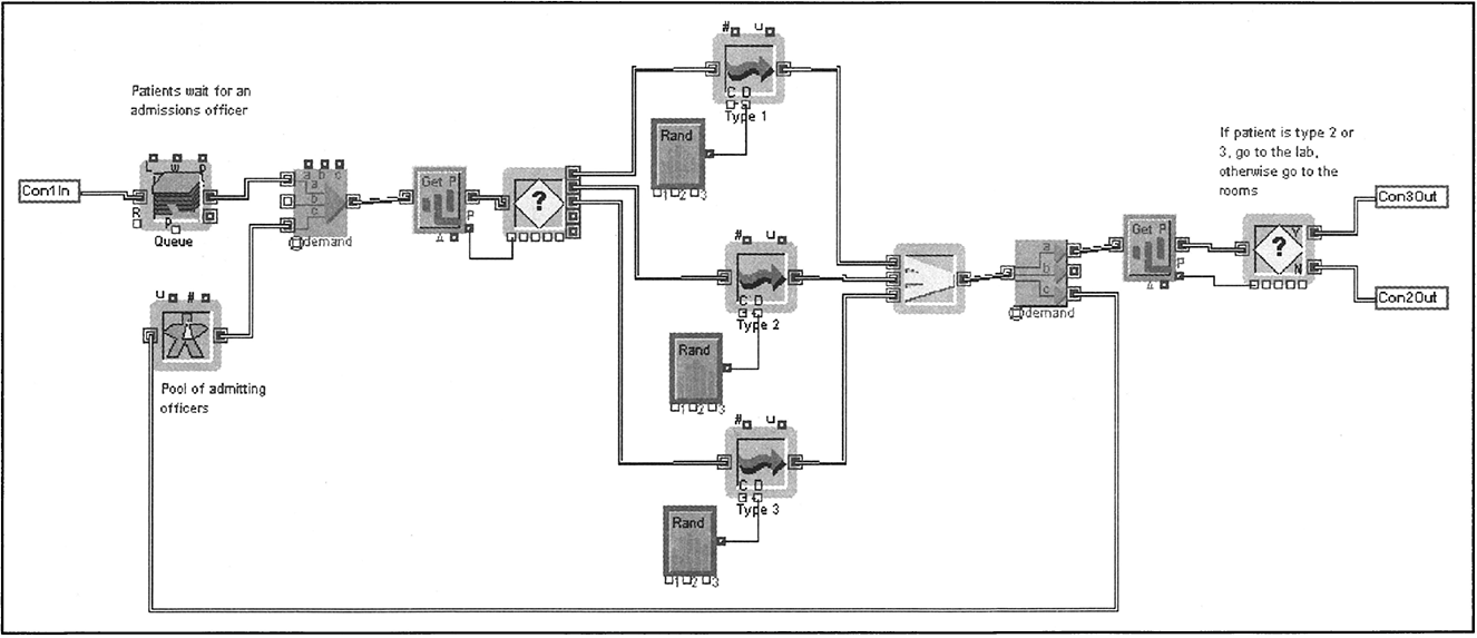
FIGURE 8.40 Admissions Block from the Admissions Model of Figure 8.38

FIGURE 8.41 Registration and Lab Block from the Admissions Model of Figure 8.38

FIGURE 8.42 Rooms Block from the Admissions Model of Figure 8.38

Table 8.5 summarizes the cycle time information for 10 days of operation of the hospital admissions process. The first column identifies the statistic. The second through the fourth columns identify the cycle time statistical value for each patient type. All values are given in minutes.
Table 8.5 indicates that all patients experience fairly long cycle times. On the average, a patient seeking admission will require approximately 2 hours to complete the process. If the patient has been preadmitted, the average time is about 40 minutes. The time values associated with Type 3 patients are all very long, with a maximum of almost 5 hours. The dispersion of the cycle time values for Type 3 patients is the largest, as indicated by the standard deviation. A frequency distribution of the cycle times for Type 1 patients, shown in Figure 8.43, revels that 75 percent of Type 1 patients experience a cycle time longer than 30 minutes. It is assumed that the hospital would like to minimize the number of Type 1 patients who experience unreasonably long cycle times, because this would discourage future patients from following the preadmission process. In other words, a patient would prefer to seek admission directly as a Type 2 patient instead of going through preadmission first as a Type 3 patient and then returning to be admitted as a Type 1 patient.
It might be possible to decrease the cycle time by adding more staff to the admissions desk, because the admitting officers have the highest average utilization of 64 percent. However, it seems more promising to explore the potential for improvement by redesigning the process instead of taking the simple approach of adding more staff.

FIGURE 8.43 Histogram of Cycle Times for Type 1 Patients
The process design project can begin with the formulation of a vision statement. A vision statement for this process might include a reference to improving service as measured by the cycle time that each patient type experiences: for instance:
The hospital admissions process will preadmit patients in an average of less than 30 minutes and never more than 45 minutes and admit patients who have been previously preadmitted in an average of less than 15 minutes and never more than 30 minutes.
The case for action in this situation might focus on the need to improve customer service in the highly competitive health care business. The following redesign opportunities are identified.
- All information about a patient can be captured at the admissions desk and distributed to the rest of the hospital via a local area network.
- All paperwork and information gathering can take place during preadmission. Therefore, the service time for Type 1 patients in the admissions desk can be minimized.
- The registration desk at the lab is unnecessary.
- It is unnecessary for patients to wait for paperwork at the nurses’ station.
- Type 2 patients could walk from the lab to the lobby to wait for an orderly instead of going back to the admissions desk.
A model of the redesigned process is depicted in Figure 8.44. The features of this model are as follows.
- The lab registration desk has been eliminated, and the person working this desk has been reassigned to the admissions desk. Patients (Types 2 and 3) are instructed to go directly to a lab technician for service. The lab technicians can access all the information about a patient from a computer terminal. The processing time at the lab remains unchanged.
- Preadmission now includes all the paperwork and information gathering necessary to admit a patient. This reduces the service time required by Type 1 patients. It is assumed that their new service time at the admissions desk is normally distributed with a mean of 5 minutes and a standard deviation of 0.5 minutes. Also, the processing times for Type 2 and Type 3 patients are reduced due to more effective (electronic) data handling. Their new processing times at the admissions desk are assumed to be 10 minutes less than the original ones.
- Type 2 patients are not required to go back to the admissions desk after completing the lab tests. Instead, they walk directly from the lab to the lobby, where they wait for an orderly to take them to their floor.
- Patients do not have to wait for paperwork at the nurses’ station. All information is available through the local area network.
Table 8.6 summarizes the results of simulating 10 days of operation of the redesigned process. The cycle time statistics show the improvement achieved with the redesigned process.
The new process is better than the original in terms of the specified (technical) measure of performance. The cycle time statistics approximate the goals specified in the vision statement. Although average max and min values are informative, a better picture of the current situation is obtained with a cumulative frequency percentage chart. Table 8.7 shows the cumulative frequency associated with the cycle times of Type 1 patients. Note that fewer than 2 percent of the Type 1 patients experience more than 14 minutes of cycle time under the new design.


TABLE 8.7 Frequency Distribution of Cycle Times for Type 1 Patients

A common managerial concern is the trade-off between customer service and the cost of installing the new local area network. One possible cost-savings strategy is to reduce the staff by operating with two admissions officers as in the original system. The cycle time statistics must be recomputed to figure out how close they are to the numerical goals specified in the vision statement.
8.13 Summary
This chapter introduced a number of modeling concepts to take advantage of the power of discrete-event simulation. Focus was placed on Extend features that are linked directly with the modeling of business processes. The chapter showed how to translate static representation of processes (flowcharts) into dynamic simulation models. In particular, it showed how to model multiple and parallel paths, priority queues, blocking, balking, and reneging. Another main goal of this chapter was to show how to conduct cycle time analysis using the Timer block to collect cycle time data. This analysis is an expansion of the one conducted in Chapter 5, where the processing times were considered deterministic. The Labor Pool block was used to perform capacity analysis and identify bottlenecks. This also represents an extension of the analysis introduced in Chapter 5 for the deterministic case.
The chapter concludes with two case studies that illustrate how simulation can be used to improve processes. The exercises that follow in Section 8.15 reinforce the modeling concepts and Extend features introduced in this and the previous chapter. Therefore, it is a good idea to be familiar with the material in both chapters before attempting to work on some of the more elaborate problems, such as those labeled as projects.
8.14 References
Imagine That Inc. 2003. Extend User’s Guide, version 6.www.imaginethatinc.com.
Nyamekye, K. 2000. New tool for business process re-engineering. IIE Solutions 32(3): 36-41.
8.15 Discussion Questions and Exercises
- Measuring Cycle Times of Different Types of Jobs—Three types of jobs arrive to a process at a rate of four jobs per hour. The interarrival times are exponentially distributed. The arrivals are not equally likely for each job type. Typically, 40 percent of the jobs are type I,35 percent are type II, and 25 percent are type III. It can be assumed that all of the processing times are exponentially distributed; however, the mean times depend on the job type. Table 8.8 shows the mean processing time for the activities associated with each job type. (All times are given in minutes.)
A flowchart of the process is depicted in Figure 8.45. Note that type I jobs are routed through activities B and C, and job types II and III are routed through activities D and E.
The percentage of rework also depends on the job type. About 5 percent of the type I jobs are reworked, about 4 percent of the type II jobs are reworked, and about 6 percent of the type III jobs are reworked. In terms of resources, the process has three types of workers. Five superworkers can handle any job; therefore, managers employ them to work on activities A, F, or G. Three type I specialists can handle only type I jobs; therefore, management employs them to work on activities B and C. Finally, three type II and III specialists can handle only type II and type III jobs; therefore, management employs them to work on activities D and E.
- Develop a simulation model for this process.
- Run the simulation for 250 hours to generate approximately 1,000 job arrivals and collect data on cycle times for each job type separately.
- Assess the performance of the process based on your analysis in part b.
- Investigating the Effect of Pooling Resources—Three types of jobs arrive to a process at a rate that randomly varies between two and five jobs per hour; that is, the interarrival times are governed by a uniform distribution with mean equal to three and a half jobs per hour. The process is currently configured in a way such that each arrival is sent to a team of specialists according to the type of job. Each team consists of three members. A team performs three activities in order to complete each job, and any team member can work on any of the three activities (A, B, or C). Figure 8.46 shows a flowchart of the process.
TABLE 8.8 Mean Processing Times for Three Different Job Types


FIGURE 8.45 Measuring Cycle Times of Different Types of Jobs
The arrivals are not equally likely for each job type. Typically, 30 percent of the jobs are type 1,35 percent are type 2, and 35 percent are type 3. Processing times (in minutes) associated with the activities depend on the job type and are summarized in Table 8.9.
Management is concerned with the current performance of the process and is considering cross training the teams so team members can work on any job type.
- Develop a simulation model of this process that can be used to model one day of operation; that is, one run of the model will consist of 8 hours of operation.
- Use your model to assess performance with the following measures: cycle times, resource utilization, and overtime (the time needed to finish all jobs after the process closes). Simulate 10 days of operation to collect data for your analysis.
- Assume that the teams are cross trained and that all nine people can perform any of the activities in the process. Compare this design with the original process using the measures in part b.
- Investigating the Effect of Rework Rates—A proposed business process consists of five serial workstations. One case worker is positioned in each workstation. The processing times at each workstation are exponentially distributed with mean values of 11, 10, 11, 11, and 12 minutes, respectively. The interarrival times are uniformly distributed between 13 and 15 minutes. The workstations have an unlimited queuing capacity, and it is assumed that the downstream transfer time is negligible. The unique aspect of this process is that between workstations 2 and 5, it is possible that the job will need to be reprocessed by the workstation immediately preceding the current one. For example, after workstation 3, it is possible that the job will be sent back to the queue in workstation 2. When this occurs, the transfer requires 3 minutes. The probability of rework remains the same regardless of the number of times a job is sent back for reprocessing. The rework probability is considered to be the same for all workstations and is currently estimated to be between,5 percent and 10 percent.

FIGURE 8.46 Investigating the Effect of Pooling Resources
TABLE 8.9 Probability Distributions for Processing Times
 (Mean, Standard Deviation)
- Develop a simulation model of this process that is capable of running 10,000 minutes of operation.
- Run 10,000 minutes of operation for rework probabilities of 5 percent, 6 percent, 7 percent, 8 percent, 9 percent, and 10 percent. Collect cycle time data for each run.
- Construct a plot of the average cycle time (y-axis) versus the rework probability (x-axis). Also construct a plot of the maximum cycle time versus the rework probability.
- Assume that the processing times are constant. Rerun the simulation six times with the rework probabilities in part b.
- Construct plots of average cycle time and maximum cycle time versus the rework probability. Compare these plots with the ones obtained in part c.
- Assessing Process Performance—The process of insuring a property consists of four main activities: review and distribution, underwriting, rating, and policy writing. Four clerks, three underwriting teams, eight raters, and five writers perform these activities in sequence. The time to perform each activity is exponentially distributed with an average of 40 minutes, 30 minutes, 70 minutes, and 55 minutes, respectively. On the average, a total of 40 requests per day are received. Interarrival times are exponentially distributed. A flowchart of the process is depicted in Figure 8.47.
- Develop a simulation model of this process. The model should simulate 10 days of operation. Assume that work-in-process at the end of each day becomes the beginning work-in-process for the next day.
- Add data collection to calculate the following measures: resource utilization, waiting time, length of the queues, work-in-process at the end of each day, and average daily throughput (given in requests per day).
- Assess the performance of the process with the data collected in part b.
- Variable Resource Availability—Travelers arrive at the main entrance door of an airline terminal according to an exponential interarrival time distribution with a mean of 1.6 minutes. The travel time from the entrance to the check-in is distributed uniformly between 2 and 3 minutes. At the check-in counter, travelers wait in a single line until one of five agents is available to serve them. The check-in time follows a normal distribution with a mean of 7 minutes and a standard deviation of 2 minutes. Upon completion of their check-in, travelers walk to their gates.
- Create a simulation model of the check-in process.
- Run the simulation for 16 hours and collect cycle time and cycle time efficiency for each traveler. Plot a frequency distribution of these values. Create a line plot of the cycle time versus the clock and the cycle time efficiency versus the clock. Also analyze queue information.
- Assume that the 16 hours are divided into two 8-hour shifts. Agent breaks are staggered, starting at 90 minutes into each shift. Each agent is given one 15-minute break. Agent lunch breaks (30 minutes) are also staggered, starting 3.5 hours into each shift. Compare the results of this model to the results without agent breaks. Use cycle time and queue data to make the comparison.
- Multiple Queues—The order-fulfillment process of an entrepreneurial catalog business operates as follows. Orders arrive with exponential interarrival times with a mean of 10 minutes. A single clerk accepts and checks the orders and processes payment. These activities require a random time that is uniformly distributed between 8 and 10 minutes. Upon completion of these activities, orders are assigned randomly to one of two stock persons, who retrieve the orders from the warehouse. The time to retrieve an order randomly varies between 16 and 20 minutes. The stock persons retrieve only their assigned orders.

FIGURE 8.47 Assessing Process Performance
- Develop a simulation model that is capable of running 5,000 minutes of this process.
- Assess the performance of the process using measures such as cycle time, queue statistics, and resource utilization.
- A manager points out that the assignment of orders should not be made at random. Instead, the manager suggests that the next order should be assigned to the stock person with the shortest queue. He also suggests breaking ties arbitrarily. Follow these recommendations and change your model accordingly. Compare the performance of this process with the original.
- A bright young “reengineer” recommends that the company eliminate the assignment of an order to a specific stock person and allow both stock persons to select their next order from a single queue. Modify your model to simulate this suggestion. Compare the performance with the previous two configurations.
- Priority Queues—A business process consists of six activities, as shown in the flowchart of Figure 8.48. The activity times are normally distributed with mean values of 15, 10, 8, 8, 13, and 7, respectively, for activities A through F. Similarly, the standard deviations are 3, 2.5, 2, 3, 3.5, and 2.
Jobs arrive every 10 minutes on the average, with actual interarrival times following an exponential distribution. Caseworkers process the jobs. Two caseworkers can perform activities A and B. Five caseworkers can perform activities C, D, E, and F. Activity C requires two caseworkers per job, and the other activities require only one caseworker per job.
When jobs arrive, they are assigned a due time, which is calculated as follows.
Due time = arrival time + random number between 30 and 50- Develop a simulation model for this process.
- Simulate the arrival of 200 jobs (i.e., simulate the process for approximately 2,000 minutes), and collect data on the tardiness for each completed job. (Hint: Consider using the Max & Min block from the Math submenu of the Generic library to calculate tardiness. This block calculates the maximum and minimum value of up to five inputs.)
- Change the queues so jobs with the earliest completion time are given priority. Compare the process performance with the process that uses a FIFO queuing discipline. (Note that Priority queues can be used to model a priority queuing discipline. Because the item with the smallest priority value is processed first, consider assigning the due date as priority in the Import block and then choose Priority in the Stack block that simulates the queue.)
- Figure 8.49 shows the flowchart of a business process that receives an average of one job every 10 minutes with a standard deviation of 2.5 minutes. The actual interarrival times approximately follow a normal distribution. The processing times are exponentially distributed with the mean values (in minutes) shown in Table 8.10. Three teams work in this process. The teams are assigned to activities as shown in Table 8.11.
- Create a simulation model of this process.
- Simulate the process for 10 working days, where each working day consists of 8 hours.

FIGURE 8.48 Priority Queues
TABLE 8.10 Mean Values for Exercise 8

TABLE 8.11 Activity Assignments for Exercise 8

- Assess the performance of the process considering waiting times, the utilization of the teams, and the work-in-process (WIP) at the end of the 10-day period.
- Add cycle time data collection and evaluate process performance considering the distribution of cycle times.
- Refer to the grocery store described in problem 8 in Chapter 7 to answer the following questions.
- To make the model more realistic, Safeway also wants to include the time customers spend in the store walking around and picking up their groceries. Empirical investigation has shown that there are basically two types of customers, and they need to be treated somewhat differently.
Type 1: The light shopper who buys only a few items (fewer than 15)
- About 60 percent of the customers arriving to the store.
- The shopping time follows a triangular distribution with a most likely value of 5 minutes, a minimum value of 2 minutes, and a maximum value of 8 minutes.
- The service times for these customers at the checkout counter are exponentially distributed with a mean of 15 seconds.
Type 2: The heavy shopper who buys several items (more than 15)
- Represents about 40 percent of the arriving customers.
- The shopping time is triangularly distributed with a most likely value of 10 minutes, a minimum value of 5 minutes, and a maximum value of 15 minutes.
- The service times for these customers at the checkout counter are exponentially distributed with a mean of 52 seconds.
The total arrival process to the store is still a Poisson process with a mean of three customers per minute. As for the queue configuration, Safeway feels that the setup in b with one line for each checkout is better for psychological reasons; one long line might deter customers from entering the store.
Modify the simulation model developed for problem 8 in Chapter 7 to incorporate the realistic elements described previously. Analyze the performance of the current process using the performance measures discussed in problem 8 of Chapter 7 as well as the following additional measures:
- The time spent shopping (average and standard deviation).
- The number of customers (average and standard deviation).
- The separate cycle times for heavy and light shoppers (average and standard deviation).
- To improve the service for the light shoppers, Safeway is thinking about dedicating one of the checkout counters to this customer group. In other words, only light shoppers are allowed to use checkout 1. The other checkout (checkout 2) will handle heavy and light shoppers. However, empirical interviews indicate that no light shopper will choose the regular lane unless at least two more shoppers are waiting in line at the express lane. How does this design change affect the cycle times for the two customer groups and for the average customer?
- To make the model more realistic, Safeway also wants to include the time customers spend in the store walking around and picking up their groceries. Empirical investigation has shown that there are basically two types of customers, and they need to be treated somewhat differently.

8.16 Modeling, Simulation, and Design Projects
8.16.1 CREDIT APPLICATIONS
The management of a mortgage company has decided with limited information that the company can save money if it reduces its staff. Before downsizing, management asks you to model the credit application process to provide reassurance that service will not be severely affected by the reduction in staff.
The mortgage company currently employs three loan agents, two of whom perform an initial review of credit applications and a third who performs a second review of the applications that fail the initial review. The second review is performed as an attempt to correct the deficiencies by contacting the originating party. The process has the following characteristics.
- Approximately four to eight credit applications (and most likely six) arrive every hour.
- It takes 12 to 16 minutes to complete the first review.
- About 20 percent of the applications fail the first review.
- It takes 25 to 35 minutes to complete the second review.
- About 50 percent of the applications fail the second review.
Your task is to compare the performance of the current process with the performance of the process using two loan agents. For the downsized process, management wants the two remaining loan agents to work in either of the two reviewing steps; that is, the loan agents are not assigned to the first or second review step, but rather they are to perform initial or second reviews as needed.
Questions
- Create a simulation model of the current process. Use the triangular distribution to model the arrivals of credit applications and the uniform distribution for the reviewing times.
- Simulate the process for 5 working days (40 hours), and collect the following data: utilization of loan agents, waiting time, and cycle time.
- Modify the model to simulate the downsized process. Repeat question 2 for the new model. Compare the performance of the two processes by analyzing the data collected during the simulation runs.
8.16.2 X-RAY PROCESS3
The Valley of Hope Hospital wishes to improve the service level in its X-ray operation. Patients have identified the total required time as the major service level issue in this process. Management, on the other hand, is concerned with utilization of available resources. Management has created a process improvement team to study this problem. The process might be redesigned as a result of the team’s recommendations.
The team has identified as the entry point to the process the instant a patient leaves the physician’s office en route to the X-ray lab. The exit point has been defined as the instant at which the patient and the completed X ray enter the physician’s office. The team has identified 12 activities in the current process, as shown in Table 8.12. The times are given in minutes. Figure 8.50 shows a flowchart of the process. Further study reveals the information in Table 8.13 concerning resource usage in the X-ray process.
The team also has analyzed the arrival and service times in the process and has determined the following. The interarrival time is exponentially distributed with a mean time of 8 minutes. The times associated with transportation activities can be considered constant. All other activity times are exponentially distributed.
TABLE 8.12 Activities in the X-Ray Process

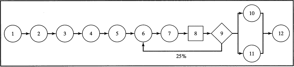
FIGURE 8.50 Flowchart for X-Ray Process

Questions
- Develop a simulation model of this process.
- Simulate 10 days of operation and compute the cycle time and resource utilization statistics. Assume a working day has 8 hours.
- Assess the performance of the process using the values calculated in question 2.
- The hospital is willing to allocate up to $2,000 per day for labor associated with the X-ray process. The hourly salaries for each labor resource are shown in Table 8.13. Management also is considering adding two more facilities, which can be a combination of X-ray labs, dark rooms, or changing rooms. Find the best configuration for the current process, assuming that management would like to minimize the maximum cycle time. The number of facilities of each type and the corresponding staffing levels define a configuration.
8.16.3 ADOPTION PROCESS IN A HUMANE SOCIETY
The purpose of this project is to redesign the pet adoption process of a Humane Society. One of the main goals of the project is the development of a simulation model of the process. The adoptions department of the Humane Society would like to use this model as a tool for evaluating the effect of proposed changes to the current pet adoption process. Management considers that the model significantly reduces the risks associated with this redesign project, because a number of what-if scenarios can be tested before implementing any changes. Furthermore, management believes that the model can help them obtain buy-in from the employees directly involved in the process.
The modeling process consists of the following steps.
- Flowcharting and analysis of the current process.
- Simulation modeling and validation.
- Performance analysis of the current process.
- Discussion of different options for redesigning the current process.
- Development of several scenarios.
- Modeling and testing of scenarios.
- Selection of final proposed process.
A task force is created to understand the current process. After several meetings of the task force, the current process is summarized as follows.
Patrons arrive to the Humane Society and look for a place to park. The arrival rate is about 10 patrons per hour, and the interarrival times follow an exponential distribution. If a patron finds the parking lot full, he or she leaves. If the parking lot is not full, the patron parks the car and enters the building (between 2 and 5 uniformly distributed minutes). Patrons then walk through the kennels (between 10 and 45 uniformly distributed minutes) and may decide to leave if they don’t find a suitable pet. About 15 percent of patrons leave at this point. If a patron finds a suitable pet, then he or she finds out what to do next to start the adoption process (between 1 and 5 uniformly distributed minutes). Patrons then count the number of people in the waiting area. (This includes people filling out the sign-in form and people waiting for a counselor.) If a patron finds fewer than 10 people in the waiting area, then he or she proceeds to sign in. If 10 people or more are in the waiting area, the patron leaves with a 70 percent probability. It takes a patron Normal(5,1) minutes to fill out the sign-in form. After signing in, patrons wait to be called to the counter to meet with a counselor. Counseling takes between 10 and 60 minutes, and 20 percent of the time patrons also must talk to a supervisor after counseling, an activity that takes Normal(15,2) minutes. After finishing counseling (or talking to the supervisor), patrons decide to stay and continue with the adoption process or leave. About 35 percent of the patrons leave at this stage of the adoption process. If a patron decides to stay, he or she must wait for a kennel technician. After a brief conversation with a kennel technician (between 2 and 5 uniformly distributed minutes), the patron and the technician visit the animals and explore options (between 5 and 45 uniformly distributed minutes). After visiting the animals, about 15 percent of the patrons decide to leave. Those who stay work with the technician to check on holds, which takes Normal(15, 3) minutes. This is necessary because some of the animals are held for people who have visited them at the Humane Society and currently are considering adoption. If there are holds (10 percent of the time), the patron is asked to return later. If there are no holds, the patron receives instructions from the kennel technician, Normal(10,2) minutes, and walks (between 1 and 2 uniformly distributed minutes) to meet with a counselor. A counselor and the patron fill out the adoption contract (between 10 and 45 uniformly distributed minutes). After the contract is signed, the health of the animal is checked (5 exponentially distributed minutes). After the health check is complete, the patron walks to the car with his or her pet and leaves (between 2 and 5 uniformly distributed minutes).
Note: A processing time given as a range of numbers is assumed to follow a uniform distribution. For example, if the time is between 10 and 45 minutes, the actual time follows a uniform distribution with a minimum value of 10 minutes and a maximum value of 45 minutes. Also, a processing time of Normal(15,3) minutes means that the actual time follows a normal distribution with a mean of 15 minutes and a standard deviation of 3 minutes.
The current process operates 10 hours per day and utilizes the following resources:
30 parking spaces
8 counselors
1 supervisor
5 kennel technicians
1 veterinarian
It is assumed that the process is empty when the doors open every morning. Also, the doors are closed after 10 hours, but personnel stay until the last patron leaves the building. Working time beyond 10 hours is considered overtime.
PART I
- Draw a flowchart of the current process.
- Create a simulation model of the current process.
- Run 30 days of operation (using 55 for the Random Seed Number).
- Analyze the performance of the system according to cycle time, resource utilization, ratio of number of adoptions per number of arrivals, and daily overtime.
The report for Part I of this project consists of an executive summary with the objectives and main findings. The supporting materials should include a flowchart of the current process, a printout of the simulation model (i.e., an annotated task network), and the following charts and tables:
- A frequency distribution of the cycle times observed during the 30-day simulation.
- A table of daily resource utilization with five columns, one for each resource, and 30 rows, one for each day. Three additional rows should contain the minimum, the average, and the maximum utilization for each resource type.
- A table with 30 rows, one for each day, and two columns, one for the daily ratio of number of adoptions per number of arrivals and one for the daily overtime. Three additional rows should contain the minimum, the average, and the maximum overtime and the adoption ratio.
PART II
- Discuss different options for redesigning the current process. For example, consider eliminating activities or performing some activities in parallel.
- Develop a redesign scenario.
- Model a redesigned process.
- Predict the performance of the redesigned process in terms of cycle time, resource utilization, ratio of adoptions to patron arrivals, and daily overtime.
The report for Part II of this project consists of an executive summary with objectives, methodology, main findings, and recommendations. The supporting materials should be the same as in the report for Part I.
8.16.4 INTERNET ORDERING PROCESS
The management of a software company wants to study the performance of the company’s Web order processing. The interarrival times of orders are exponentially distributed with a mean of 7 minutes. The orders arrive in the form of e-mail. Upon arrival, a clerk looks for the buyer’s name in the company’s database. The time required to look for a name in the database is uniformly distributed between 20 and 45 seconds. If the buyer is not in the database, the clerk enters the buyer’s information, which includes name, address, phone number, and e-mail address. The time required to enter the buyer’s information in the database is uniformly distributed between 10 and 30 seconds. Approximately 60 percent of the time, the buyer’s name is not in the database. Some orders are for an upgrade of the software, and the others are from first-time buyers. For all practical purposes, it takes no time to figure out whether an order is for an upgrade or from a first-time buyer. Approximately 30 percent of the orders are for upgrades. If the order is for an upgrade, then the clerk simply enters a code in the electronic purchase order (PO), created when the buyer’s name was entered or found in the database. (This code is later e-mailed to the customer, so he or she can download an upgrade from the company’s Web site.) Entering the code requires an exponentially distributed time with a mean of 2 minutes, because the clerk needs to verify the customer’s current software version and platform. After entering the code, the electronic PO goes to accounting.
When the order is from a first-time buyer, the clerk checks whether the buyer wants the CD version with printed documentation or whether he or she prefers to download the software from the company’s Web site. This requires an exponentially distributed time with a mean of 1 minute because sometimes this information has been misplaced. About 70 percent of the buyers prefer the CD version. When the CD version is preferred, the clerk needs to retrieve it from the storage room. This activity requires a normally distributed time with a mean of 5 minutes and a standard deviation of 1. The clerk then prepares the software for shipping, which takes between 3 and 6 minutes (uniform distribution). If the buyer prefers to download the software, the clerk enters an appropriate code in the electronic PO. Entering the code requires an exponentially distributed time with a mean of 1 minute, because a computer program sometimes is slow at generating a license for each customer.
Purchase orders for upgrades and first-time buyers go to accounting after a clerk has either entered a code for downloading or prepared the CD version for shipping. Accounting personnel charge the purchase to a credit card (Exponential distribution with a mean of 2 minutes) and prepare the invoice (Normal distribution with a mean of 1 minute and a standard deviation of 12 seconds). Finally, the accounting personnel mail the software or e-mail the access code with the invoice. This activity requires a uniformly distributed time between 45 and 90 seconds.
Currently, the company employs two people for this process: one clerk for the initial processing and one person in charge of the accounting. However, management is considering adding one person to the process and would like to use simulation to determine where to add this new employee to obtain the maximum customer service benefit.
Questions
- The first task is to understand this process, so you should develop a flowchart. This chart should be the first exhibit in your written report.
- Using the flowchart as a guideline, develop a simulation model of this process. Because only two resource types are in this process (the clerks and the accounting personnel), your model should have only two queues. Include an exhibit consisting of the simulation model.
- Set the random seed value to 34 in the Simulation Setup of the Run menu. Run the model for 15 working days and collect the waiting time at the queues, cycle time, resource utilization, and work-in-process. (A working day consists of 8 hours.)
- Discuss the performance of the current process based on the collected data. Include the following exhibits to support your arguments: queue statistics, line graphs of resource utilization, a histogram of cycle times, and the WIP value at the end of the 15 days.
- Identify the bottleneck and add the new employee to the bottleneck. Compare the utilization of clerks and accounting personnel before and after adding the new employee. Also compare the frequency distribution of cycle times before and after adding the new employee. Include line graphs for the utilization of resources after adding the new employee and a histogram of cycle times.
8.16.5 AN ASSEMBLY FACTORY
The LeedsSim factory is a traditional assembly facility working as a subcontractor to the telecommunications industry. Their main product is a specialized switchboard cabinet used in the third-generation network base stations. The company has been successful on the sales side, and with the 3G expansion taking off in Europe, the orders are piling up. Unfortunately, the operations department has had some problems with reaching the desired (and necessary) productivity levels. Therefore, they have decided to seek your help to create a simulation model of the involved processes as a first step to analyze and improve the process design.
To find the right level of detail in the model description, they want to start with a simple model and then successively add more details until a suitable model with the right level of complexity is obtained. The simulation should be run over a 1-month (4-week) period of 8-hour workdays. A schematic flowchart of the manufacturing process is shown in Figure 8.51.
After the cabinets are completed and inspected, the finished cabinets leave the factory. It is noteworthy that each workstation can handle only one item at a time. Workstations 1 through 4 cannot store items. Each cabinet that is made requires one unit each of five sorts of components/raw materials delivered to the inbound storage area. Workstation 1 requires one unit each of raw materials 1 and 2, workstation 2 requires one unit of raw material 3, and workstation 3 requires one unit each of raw materials 4 and 5. Table 8.14 specifies the estimated processing times in workstations 1 through 5, as well as the estimated inspection time.

FIGURE 8.51 Flowchart of the Production Process
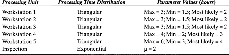
The performance measure that LeedsSim is most interested in is the number of cabinets produced in 1 month. However, they also want to keep track of the following.
- The work-in-process levels–the total as well as at different parts of the workshop, including inbound storage (the maximum, the mean, and the standard deviation).
- The cycle time, measured from the instant a component arrives to the storage area until a finished cabinet leaves the factory (both the mean and standard deviation). (Hint: Note that all components for a particular cabinet have the same cycle time.)
- Utilizations of workstations and equipment such as the forklift truck.
Questions
- The raw material arrives by truck once every week on Monday morning. Each shipment contains 15 units each of the five necessary components. The internal logistics within the factory are such that the transportation times for the incomplete cabinets can be neglected. However, to transport the fully assembled cabinet to and from the paint shop, a special type of forklift truck is needed. The transportation time from the assembly line to the paint shop is exponentially distributed with a mean of 45 minutes, which includes the travel time for the truck to get from its parking area to the assembly line. The transportation time between the paint shop and the inspection station at the loading dock is normally distributed with a mean of 60 minutes and a standard deviation of 15 minutes, including the travel time for the truck to get from its parking area to the paint shop. After delivery, the forklift truck always returns to the strategically located parking area to get new instructions. The travel time, without load, back from the inspection station as well as the paint shop is 20 minutes (constant). One forklift truck is available at the moment. For this first model, assume that all painted cabinets pass inspection so no rework occurs.
- Run the simulation once with random seed = 5.
How many cabinets are being produced?
How is the WIP situation?
What does a plot over the storage inventory levels tell us?
Where is the bottleneck?
- Run the simulation 15 times with different random seeds.
How many cabinets are being produced on average?
What is the standard deviation?
How is the WIP situation?
Where is the bottleneck?
(Hint to collect the data and analyze it efficiently: Use the Resource, Activity, and Queue statistics blocks, check Append New Updates, and click on Confidence Interval. For the number of units produced, use a Mean and Variance block, connect it to the exit block, and check the dialogue options Calculate for Multiple Simulations, and Use Number of Inputs-1.)
- Run the simulation once with random seed = 5.
- In reality, only 75 percent of the painted cabinets pass the inspection. If a cabinet fails the inspection, it needs to be transported back to the paint shop to be repainted. The transportation time (including travel time for the truck to get to the inspection site) is the same as in the opposite direction (normally distributed with a mean of 60 minutes and a standard deviation of 15 minutes). The forklift truck will always go back to the parking area after a completed mission. The travel time without load from the paint shop to the parking area is constantly 20 minutes. When arriving to the paint shop, repainting has higher priority than the ordinary paint jobs and follows an exponential distribution with a mean of 2 hours. Inspecting the reworked cabinets is no different from inspecting nonreworked cabinets. How does the introduction of these features affect the performance measures?
- Run the simulation once with random seed = 5.
How many cabinets are being produced?
How is the WIP situation?
Where is the bottleneck?
- Run the simulation 15 times with different random seeds.
How many cabinets are being produced on average?
What is the standard deviation?
How is the WIP situation?
Where is the bottleneck?
- Run the simulation once with random seed = 5.
- Based on your understanding of the process, suggest a few design changes and try them out. What is your recommendation to LeedsSim regarding how to improve their operations?
- In this model, we have started to collect statistics and count units produced from time 0, meaning we assume the system is empty when we start. It would be more accurate to run the system for a warm-up period, say 1 week, before starting to collect data. Implement this and see the difference. Does it change your conclusions?