CHAPTER 6
Introduction to Queuing and Simulation
The process models analyzed in Chapters 4 and 5 have one thing in common: They assume that activity times and demand are deterministic and constant; that is, that they are known with certainty. In reality, an element of variability will always exist in the time it takes to perform a certain task and in the demand for service. In situations where the variability is small, deterministic models of the type studied in Chapters 4 and 5 might be an adequate way of describing a process. However, in situations with more accentuated variability, these models do not suffice. In fact, the variability itself is often one of the most important characteristics to capture in the model of a process.
Consider, for example, the checkout process at a grocery store where one of the main design issues is to avoid long lines. Customers arrive at the checkout stations with their items so they can pay and leave. Each cashier scans the items, bags them, and collects payment from the customer. The time it takes to service a customer depends on the amount and type of groceries and the form of payment used; therefore, it varies from customer to customer. In addition, the number of customers per time unit that arrive at the cashier’s station, meaning the demand for service, is highly uncertain and variable. Applying a deterministic model to describe this process, using only the average service time and the average number of customer arrivals per time unit, fails to capture the variability and explain why queues are forming. This is because the deterministic model assumes that it always takes exactly the same amount of time for a cashier to serve a customer, and that customers arrive at constant intervals. Under these assumptions, it is easy to determine the number of cashiers needed to avoid queues. However, the fact that everyone has waited at a cashier’s station indicates that this is too simplistic of a way to describe the complex reality. Variability makes it difficult to match demand and capacity in such a way that queues are avoided.
The focus of this chapter is the incorporation of variability into models of business processes. These types of models, known in the literature as stochastic models, enable us to evaluate how the process design decisions affect waiting times, queue lengths, and service levels. An important difference compared to the deterministic models that have been considered so far is that in the stochastic models the waiting time is no longer an input parameter; it is the result of the specified process time and the demand pattern. Because eliminating non-value-adding waiting time is an important objective when designing a new business process (see, for example, Section 1.1), the usefulness of stochastic models in process design is obvious.
The modeling approaches that will be explored in this chapter belong to two distinct groups: analytical queuing models stemming from the field of mathematical queuing theory, and simulation models, which are in their nature experimental and in this case computer based. Chapters 7 through 10 also address the simulation modeling approach. The reason for considering these two approaches is that they offer different advantages to the process designer. The analytical queuing models express important performance characteristics in mathematical formulae and are convenient to use when the necessary conditions are in place. The drawback is that these conditions can be restrictive with regard to the process structure and the representation of variability in the models. The simulation models are more flexible, but they usually take more time to set up and run, in addition to requiring a computer with the appropriate software. Because the simulation models are experimental, they also require statistical analysis of input and output data before obtaining the appropriate information on performance characteristics sought by the process designer. This chapter investigates the technical aspects of these two modeling approaches. However, before getting into the modeling details, it is important to understand why variability in process parameters is such an important issue from an operational and an economic perspective.
From an operational perspective, the main problem with variability in processing times, demands, and capacity is that it leads to an unbalanced use of resources over time, causing the formation of waiting lines. This will be referred to loosely as a capacity-planning problem. The core of this problem is that queues (or waiting lines) can arise at any given time when the demand for service exceeds the resource capacity for providing the service. This means that even if the average demand falls well below the average capacity, high variability will lead to instances when the demand for service exceeds the capacity and a queue starts to form. This explains the formation of waiting lines in the grocery store example. On the other hand, in some instances the capacity to provide service will greatly exceed the demand for service. This causes the queue to decrease. Moreover, if no queue exists at all, the resource providing the service will be idle. At a grocery store, even if a cashier has nothing to do for long periods during the day, the arrival of a customer with a full cart could initiate a queue.
At this point, it is important to recognize that queues concern individuals as well as documents, products, or intangible jobs such as blocks of information sent over the Internet. However, the issues with waiting in line are particularly important in service industries where the queue consists of people waiting for service. The reason is that, as opposed to objects or pieces of information, people usually find waiting frustrating, and they often give an immediate response regarding their dissatisfaction.
From an economic perspective, the capacity-planning problem caused by high variability in demand and process times comes down to balancing the cost of having too much capacity on certain occasions against the cost associated with long waiting lines at other times. The cost of delays and waiting can take on many different forms including the following.
- The social costs of not providing fast enough care at a hospital.
- The cost of lost customers who go elsewhere because of inadequate service.
- The cost of discounts because of late deliveries.
- The cost of goodwill loss and bad reputation affecting future sales.
- The cost of idle employees who have to wait for some task to be completed before they can continue their work.
Ultimately, these costs will affect the organization, even though the impact sometimes might be hard to quantify. The cost of excessive capacity is usually easier to identify. Primarily, it consists of the fixed and variable costs of additional and unused capacity, including increased staffing levels. Returning to the grocery store example, the store must balance the cost of hiring additional cashiers and installing more checkout stations against the cost of lost customers and lower sales revenues due to long queues and waiting times at the checkout stations.
Figure 6.1 depicts the economic tradeoff associated with the capacity-planning problem. The x-axis represents the service capacity expressed as the number of jobs per unit of time the system can complete on average1. The y-axis represents the total costs associated with waiting and providing service. The waiting cost reflects the cost of having too little service capacity, and the service cost reflects the cost of acquiring and maintaining a certain service capacity.
It follows that in order to arrive at design decisions that will minimize the total costs, the first step is to quantify the delay associated with a certain capacity decision. Second, this delay needs to be translated into monetary terms to compare this to the cost of providing a certain service capacity. This chapter investigates models that deal with both of these issues.
Section 6.1 specifies a conceptual model over the basic queuing process and defines what a queuing system is. This section also discusses strategies that are often used in service industries for mitigating the negative effects of making people wait in line. The conceptual model for the basic queuing process serves as a basis for the analytical queuing models investigated in Section 6.2 and for the general understanding of the simulation models in Section 6.3. Finally, a summary and some concluding remarks are provided in Section 6.4.

FIGURE 6.1 Economic Tradeoff Between Service Capacity and Waiting Times
6.1 Queuing Systems, the Basic Queuing Process, and Queuing Strategies
Queuing processes, queuing systems, and queuing models might appear to be abstract concepts with limited practical applicability, but nothing could be further from the truth. Wherever people go in their daily lives, they encounter simple queuing systems and queuing processes (e.g. at the bank, in the grocery store, or when calling for a taxi, going to the doctor, eating at a restaurant, buying tickets to the theater, or taking the bus). In simple terms, an elementary queuing system consists of a service mechanism with servers providing service and one or more queues of customers or jobs waiting to receive service. The queuing process, on the other hand, describes the operations of the queuing system; that is, how customers arrive at the queuing system and how they proceed through it. The queuing system is an integral part of the queuing process. Noting the subtle distinction between a queuing process and a queuing system will prove useful when discussing detailed modeling issues. However, in practical situations and in higher-level discussions, these two terms are often interchangeable. Going back to the definition of a business process as a network of connected activities and buffers (see Section 1.1), a business process can be interpreted as a network of queuing processes or elementary queuing systems.
To expand the frame of reference regarding queuing systems and to make this concept more concrete, one can look at a number of examples of real-world queuing systems that can be broadly classified as commercial, transportation, business-internal, and social service systems.
Many of the queuing systems we encounter daily are commercial service systems, whereby a commercial organization serves external customers. Often the service is a personal interaction between the customer and an employee, but in some cases, the service provider might be a machine. Typically, customers go to a fixed location to seek service. Examples include a dentist’s office (where the server is the dentist), banks, checkout stations at supermarkets or other stores, gas stations, and automated teller machines. However, the server also can travel to the customer. Examples include a plumber or cable company technician visiting the customer’s home to perform a service.
The class of transportation service systems represents situations where vehicles are either customers or servers. Examples where vehicles are customers include cars and trucks waiting at tollbooths, railroad crossings, or traffic lights; trucks or ships waiting to be loaded; and airplanes waiting to access a runway. Situations where vehicles constitute the servers in a queuing system include taxicabs, fire trucks, elevators, buses, trains, and airplanes transporting customers between locations.
In business-internal service systems, the customers receiving service are internal to the organization providing the service. This definition includes inspection stations (the server), materials handling systems like conveyor belts, maintenance systems where a technician (the server) is dispatched to repair a broken machine (the customer), and internal service departments like computer support (the server) servicing requests from employees (the customers). It also includes situations where machines in a production facility or a supercomputer in a computing center process jobs.
Finally, many social service systems are queuing systems. In the judicial process, for example, the cases awaiting trial are the customers and the judge and jury is the server. Other examples include an emergency room at a hospital, the family doctor making house calls, and waiting lists for organ transplants or student dorm rooms.
This broad classification of queuing systems is not exhaustive and it does have some overlap. Its purpose is just to give a flavor of the wide variety of queuing systems facing the process designer.
A conceptual model of the basic queuing process describes the operation of the queuing systems just mentioned and further explains the subtle distinction between a queuing process and a queuing system. It also will provide the basis for exploring the mathematical queuing models in Section 6.2 and help conceptualize the simulation models in Section 6.3. Following the discussion of the basic queuing process, Section 6.1.2 looks at some pragmatic strategies used to mitigate the negative economic impact of long waiting lines.
6.1.1 THE BASIC QUEUING PROCESS
The basic queuing process describes how customers arrive at and proceed through the queuing system. This means that the basic queuing process describes the operations of a queuing system. The following major elements define a basic queuing process: the calling population, the arrival process, the queue configuration, the queue discipline, and the service mechanism. The elements of the basic queuing process are illustrated in Figure 6.2, which also clarifies the distinction between the basic queuing process and the queuing system.
Customers or jobs from a calling population arrive at one or several queues (buffers) with a certain configuration. The arrival process specifies the rate at which customers arrive and the particular arrival pattern. Service is provided immediately when the designated queue is empty and a server (resource) is available. Otherwise, the customer or job remains in the queue waiting for service.
In service systems in which jobs are actual customers (i.e., people), some may choose not to join the queue when confronted with a potentially long wait. This behavior is referred to as balking. Other customers may consider, after joining the queue, that the wait is intolerable and renege (i.e., they leave the queue before being served). From a process performance perspective, an important distinction between balking and reneging is that the reneging customers take up space in the queue and the balking customers do not. For example, in a call center, the reneging customers will accrue connection costs as long as they remain in the queue.

FIGURE 6.2 The Basic Queuing Process and the Queuing System
When servers (resources) become available, a job is selected from the queue and the corresponding service (activity) is performed. The policy governing the selection of a job from the queue is known as the queue discipline. Finally, the service mechanism can be viewed as a network of service stations where activities are performed. These stations may need one or more resources to perform the activities, and the availability of these resources will result in queues of different lengths.
This description of a queuing process is closely related to the definition of a general business process given in Section 1.1. In fact, as previously mentioned, a general business process can be interpreted as a network of basic queuing processes (or queuing systems).
Due to the importance of the basic queuing process, the remainder of this section is devoted to a further examination of its components.
The Calling Population
The calling population can be characterized as homogeneous (i.e., consisting of only one type of job), or heterogeneous, consisting of different types of jobs. In fact, most queuing processes will have heterogeneous calling populations. For example, the admissions process at a state university has in-state and out-of-state applicants. Because these applications are treated differently, the calling population is not homogeneous. In this case, the calling population is divided into two subpopulations.
The calling population also can be characterized as infinite or finite. In reality, few calling populations are truly infinite. However, in many situations, the calling population can be considered infinite from a modeling perspective. The criterion is that if the population is so large that the arrival process is unaffected by how many customers or jobs are currently in the queuing system (in the queue or being served), the calling population is considered infinite. An example of this is a medium-sized branch office of a bank. All potential customers who might want to visit the bank define the calling population. It is unlikely that the number of customers in the bank would affect the current rate of arrivals. Consequently, the calling population could be considered infinite from a modeling perspective.
In other situations, the population cannot be considered infinite. For example, the mechanics at a motorized army unit are responsible for maintenance and repair of the unit’s vehicles. Because the number of vehicles is limited, a large number of broken down vehicles in need of repair implies that fewer functioning vehicles remain that can break down. The arrival process—vehicles breaking down and requiring the mechanic’s attention—is most likely dependent on the number of vehicles currently awaiting repair (i.e., in the queuing system). In this case, the model must capture the effect of a finite calling population.
The Arrival Process
The arrival process refers to the temporal and spatial distribution of the demand facing the queuing system. If the queuing process is part of a more general business process, there may be several entry points for which the arrival processes must be studied. The demand for resources in a queuing process that is not directly connected to the entry points to the overall business process is contingent on how the jobs are routed through this process. That is, the path that each type of job follows determines which activities are performed most often and therefore which resources are most needed.
The arrival process is characterized by the distribution of interarrival times, meaning the probability distribution of the times between consecutive arrivals. To determine these distributions in practice, data need to be collected from the real-world system and then statistical methods can be used to analyze the data and estimate the distributions. The approach can be characterized in terms of the following three-step procedure.
- Collect data by recording the actual arrival times into the process.
- Calculate the interarrival times for each job type.
- Perform statistical analysis of the interarrival times to fit a probability distribution.
Specific tools to perform these steps are described in Chapter 9.
The Queue Configuration
The queue configuration refers to the number of queues, their location, their spatial requirements, and their effect on cuused queue configurationsstomer behavior. Figure 6.3 shows two commonly used queue configurations: the single-line versus the multiple-line configuration.
For the multiple-line alternative (Figure 6.3a), the arriving job must decide which queue to join. Sometimes the customer, like in the case of a supermarket, makes the decision. However, in other cases this decision is made as a matter of policy or operational rule. For example, requests for technical support in a call center may be routed to the agent with the fewest requests at the time of arrival. In the single-line configuration (Figure 6.3b), all the jobs join the same line. The next job to be processed is selected from the single line.
Some advantages are associated with each of these configurations. These advantages are particularly relevant in settings where the jobs flowing through the process are people. The multiple-line configuration, for instance, has the following advantages.

FIGURE 6.3 Alternative Queue Configurations
- The service provided can be differentiated. The use of express lanes in supermarkets is an example. Shoppers who require a small amount of service can be isolated and processed quickly, thereby avoiding long waits for little service.
- Labor specialization is possible. For example, drive-in banks assign the more experienced tellers to the commercial lane.
- The customer has more flexibility. For example, the customer in a grocery store wIth several check out stations has the option of selecting a particular cashier of preference.
- Balking behavior may be deterred. When arriving customers see a long, single queue snaked in front of a service, they often interpret this as evidence of a long wait and decide not to join the line.
The following are advantages of the single-line configuration.
- The arrangement guarantees “fairness” by ensuring that a first-come-first-served rule is applied to all arrivals.
- Because only a single queue is available, no anxiety is associated with waiting to see if one selected the fastest line.
- With only one entrance at the rear of the queue, the problem of cutting in is resolved. Often the single line is roped into a snaking pattern, which makes it physically more difficult for customers to leave the queue, thereby discouraging reneging. Reneging occurs when a customer in line leaves the queue before being served, typically because of frustration over the long wait.
- Privacy is enhanced, because the transaction is conducted with no one standing immediately behind the person being served.
- This arrangement is more efficient in terms of reducing the average time that customers spend waiting in line.
- Jockeying is avoided. Jockeying refers to the behavior of switching lines. This occurs when a customer attempts to reduce his or her waiting time by switching lines as the lines become shorter.
The Queue Discipline
The queue discipline is the policy used to select the next job to be served. The most common queue discipline is first-come-first-served (FCFS), also known as first-in-first-out (FIFO). This discipline, however, is not the only possible policy for selecting jobs from a queue. In some cases, it is possible to estimate the processing time of a job in advance. This estimate can then be used to implement a policy whereby the fastest jobs are processed first. This queue discipline is known as the shortest processing time first (SPT) rule, as discussed in Chapter 4. Other well-known disciplines are last-in-first-out (LIFO) and longest processing time first (LPT).
In addition to these rules, queue disciplines based on priority are sometimes implemented. In a medical setting, for example, the procedure known as triage is used to give priority to those patients who would benefit the most from immediate treatment. An important distinction to be made in terms of priority disciplines is that between nonpreemptive and preemptive priorities. Under a nonpreemptive priority discipline, a customer or job that is currently being served is never sent back to the queue in order to make room for an arriving customer or job with higher priority. In a preemptive discipline, on the other hand, a job that is being served will be thrown back into the queue immediately to make room for an arriving job with higher priority.
The preemptive strategy makes sense, for example, in an emergency room where the treatment of a sprained ankle is interrupted when an ambulance brings in a cardiac arrest patient and the physician must choose between the two. The drawback with the preemptive discipline is that customers with low priorities can experience extremely long waiting times.
The nonpreemptive strategy make sense in situations where interrupting the service before it is finished means that all the work put in is wasted and the service needs to be started from scratch when the job eventually rises in importance again. For example, if a limousine service is driving people to and from an airport, it makes little sense to turn the limousine around in order to pick up a VIP client at the airport just before it reaches the destination of its current passenger.
In many cases in which the customers are individuals, a preemptive strategy can cause severe frustration for low-priority customers. A nonpreemptive approach is often more easily accepted by all parties. Note that queuing disciplines in queuing theory correspond to dispatching rules in sequencing and scheduling (see Section 4.2.6).
The Service Mechanism
The service mechanism is comprised of one or more service facilities, each containing one or more parallel service channels referred to as servers. A job or a customer enters a service facility, where one server provides complete service. In cases where multiple service facilities are set up in series, the job or customer might be served by a sequence of servers. The queuing model must specify the exact number of service facilities, the number of servers in each facility, and possibly the sequence of service facilities a job must pass through before leaving the queuing system. The time spent in a service facility, meaning time in one particular server or service station, is referred to as the service time. The service process refers to the probability distribution of service times associated with a certain server (possibly different across different types of customers or jobs). Often it is assumed that the parallel servers in a given service facility have the same service time distribution. For example, in modeling the parallel tellers in a bank, it is usually reasonable to assume that the service process is the same for all tellers. Statistically, the estimation of the service times can be done in a similar way as the estimation of interarrival times. See Chapter 9.
The design of the service mechanism and queues together with the choice of queuing disciplines result in a certain service capacity associated with the queuing system. For example, the service mechanism may consist of one or more service facilities with one or more servers. How many is a staffing decision that directly affects the ability of the system to meet the demand for service. Adding capacity to the process typically results in decreasing the probability of long queues and, therefore, decreases the average waiting time of jobs in the queue. Often, the arrival process is considered outside the decision maker’s control. However, sometimes implementing so-called demand management strategies is an option. This can involve working with promotional campaigns, such as “everyday low prices” at Wal-Mart, to encourage more stable demand patterns over time. These types of activities also go by the name of revenue management.
6.1.2 STRATEGIES FOR MITIGATING THE EFFECTS OF LONG QUEUES
In some situations, it might be unavoidable to have long waiting lines occasionally. Consider, for example, a ski resort. Most people arrive in the morning to buy tickets so they can spend the whole day on the slopes. As a result, lines will form at the ticket offices early in the day, no matter how many ticket offices the resort opens.
A relevant question is how the process designer or process owner might mitigate the negative economic effects of queues or waiting lines that have formed. This is of particular interest in service systems that want to avoid balking and reneging. Commonly used strategies are based on the ideas of concealing the queue, using the customer as a resource, making the wait comfortable, distracting the customer’s attention, explaining the reasons for the wait, providing pessimistic estimates of remaining waiting time, and being fair and open about the queuing discipline.
An often-used strategy for minimizing or avoiding lost sales due to long lines is to conceal the queue from arriving customers (Fitzsimmons and Fitzsimmons, 1998). Restaurants achieve this by diverting people to the bar, which in turn has the potential to increase revenues. Amusement parks such as Disneyland require people to pay for their tickets outside the park, where they are unable to observe the waiting lines inside. Casinos “snake” the waiting line for nightclub acts through the slot machine area, in part to hide its true length and in part to foster impulsive gambling.
In some cases, a fruitful approach is to consider the customer as a resource with the potential to be part of the service delivery. For example, a patient might complete a medical history record while waiting for a doctor, thereby saving the physician valuable time. This strategy increases the capacity of the process while minimizing the psychological effects of waiting.
Regardless of other strategies, making the customer’s wait comfortable is necessary to avoid reneging and loss of future sales due to displeased and annoyed customers. This can be done in numerous ways, such as by providing complementary drinks at a restaurant or by having a nicely decorated waiting room with interesting reading material in a doctor’s office.
Closely related to this idea is distracting the waiting customers’ attention, thereby making the wait seem shorter than it is. Airport terminals, for instance, have added public TV monitors, food courts, and shops.
If an unexpected delay occurs, it is important to inform the customer about this as soon as possible, but also to explain the reason for the extra wait. The passengers seated on a jumbo jet will be more understanding if they know that the reason for the delay is faulty radio equipment. Who wants to fly on a plane without a radio? However, if no explanation is given, attitudes tend to be much less forgiving because the customers feel neglected and that they have not been treated with the respect they deserve. Keeping the customers informed is also a key concept in all industries that deliver goods. Consider, for example, the tracking systems that FedEx and other shipping companies offer their customers.
To provide pessimistic estimates of the remaining waiting time is often also a good strategy. If the wait is shorter than predicted, the customer might even leave happy. On the other hand, if the wait is longer than predicted the customers tend to lose trust in the information and in the service.
Finally, it is important to be fair and open about the queuing discipline used. Ambiguous VIP treatment of some customers tends to agitate those left out; for example, think about waiting lines at popular restaurants or nightclubs.
6.2 Analytical Queuing Models
This section will examine how analytical queuing models can be used to describe and analyze the basic queuing process and the performance characteristics of the corresponding queuing system. The mathematical study of queues is referred to as queuing or queuing theory.
The distributions of interarrival and service times largely determine the operational characteristics of queuing systems. After all, considering these distributions instead of just their averages is what distinguishes the stochastic queuing models fromthe deterministic models in Chapters 4 and 5. In real-world queuing systems, these distributions can take on virtually any form, but they are seldom thought of until the data is analyzed. However, when modeling the queuing system mathematically, one must be specific about the type of distributions being used. When setting up the model, it is important to use distributions that are realistic enough to capture the system’s behavior. At the same time, they must be simple enough to produce a tractable mathematical model. Based on these two criteria, the exponential distribution plays an important role in queuing theory. In fact, most results in elementary queuing theory assume exponentially distributed interarrival and service times. Section 6.2.1 discusses the importance and relevance of the exponential distribution, as well as its relation to the Poisson process.
The wide variety of specialized queuing models calls for a way to classify these according to their distinct features. A popular system for classifying queuing models with a single service facility with parallel and identical servers, a single queue and a FIFO queuing discipline, uses a notational framework with the structure A1/A2/A3/A4/A5. Attributes A1 and A2 represent the probability distribution of the interarrival and service times, respectively. Attribute A3 denotes the number of parallel servers. Attribute A4 indicates the maximum number of jobs allowed in the system at the same time. If there is no limitation, A4 = ∞. Finally, attribute A5 represents the size of the calling population. If the calling population is infinite, then A5 = ∞. Examples of symbols used to represent probability distributions for interarrival and service times — that is, attributes A1 and A2 — include the following.
M = Markovian, meaning the interarrival and service times follow exponential distributions
D = Deterministic, meaning the interarrival and service times are deterministic and constant
G = General, meaning the interarrival times may follow any distribution
Consequently, M/M/c refers to a queuing model with c parallel servers for which the interarrival times and the service times are both exponentially distributed. Omitting attributes A4 and A5 means that the queue length is unrestricted and the calling population is infinite. In the same fashion, M/M/c/K refers to a model with a limitation of at most K customers or jobs in the system at any given time. M/M/c/∞/N, on the other hand, indicates that the calling population is finite and consists of N jobs or customers.
Exponentially distributed interarrival and service times are assumed for all the queuing models in this chapter. In addition, all the models will have a single service facility with one or more parallel servers, a single queue and a FIFO queuing discipline. It is important to emphasize that the analysis can be extended to preemptive and non-preemptive priority disciplines, see, for example, Hillier and Lieberman (2001). Moreover, there exist results for many other queuing models not assuming exponentially distributed service and interarrival times. Often though, the analysis of these models tends to be much more complex and is beyond the scope of this book.
This exploration of analytical queuing models is organized as follows. Section 6.2.1 discusses the exponential distribution, its relevance, important properties, and its connection to the Poisson process. Section 6.2.2 introduces some notation and terminology used in Sections 6.2.3 through 6.2.8. Important concepts include steady-state analysis and Little’s law. Based on the fundamental properties of the exponential distribution and the basic notation introduced in Section 6.2.2, Section 6.2.3 focuses on general birth-and-death processes and their wide applicability in modeling queuing processes. Although a powerful approach, the method for analyzing general birth-and-death processes can be tedious for large models. Therefore, Sections 6.2.4 through 6.2.7 explore some important specialized birth-and-death models with standardized expressions for determining important characteristics of these queuing systems. Finally, Section 6.2.8 illustrates the usefulness of analytical queuing models for making process design-related decisions, particularly by translating important operational characteristic into monetary terms.
6.2.1 THE EXPONENTIAL DISTRIBUTION AND ITS ROLE IN QUEUING THEORY
The exponential distribution has a central role in queuing theory for two reasons. First, empirical studies show that many real-world queuing systems have arrival and service processes that follow exponential distributions. Second, the exponential distribution has some mathematical properties that make it relatively easy to manipulate.
In this section, the exponential distribution is defined and some of its important properties and their implications when used in queuing modeling are discussed. The relationship between the exponential distribution, the Poisson distribution, and the Poisson process is also investigated. This discussion assumes some prior knowledge of basic statistical concepts such as random variables, probability density functions, cumulative distribution functions, mean, variance, and standard deviation. Basic books on statistics contain material related to these topics, some of which are reviewed in Chapter 9.
To provide a formal definition of the exponential distribution, let T be a random (or stochastic) variable representing either interarrival times or service times in a queuing process. T is said to follow an exponential distribution with parameter α if itsprobability density function (or frequency function), fT(t), is:

The shape of the density function fT(t) is depicted in Figure 6.4, where t represents the realized interarrival or service time.

FIGURE 6.4 The Probability Density Function for an Exponentially Distributed Random Variable T
The expression for the corresponding cumulative distribution function, FT(t), is then

To better understand this expression, recall that per definition FT(t) = P(T ≤ t), where P(T ≤ t) is the probability that the random variable T is less than or equal to t. Consequently, P(T ≤ t) = 1 − e−αt This also implies that the probability that T is greater than t, P(T > t), can be obtained as P(T > t) = 1 − P(T > t) = e−αt. Finally, it can be concluded that the mean, variance, and standard deviation of the exponentially distributed random variable T, denoted E(T), Var(T), and σT are, respectively:

Note that the standard deviation is equal to the mean, which implies that the relative variability is high.
Next, the implications of assuming exponentially distributed interarrival and service times will be examined. Does it make sense to use this distribution? To provide an answer, it is necessary to look at a number of important properties characterizing the exponential distribution, some of which are intuitive and some of which have a more mathematical flavor.
First, from looking at the shape of the density function fT(t) in Figure 6.4, it can be concluded that it is decreasing in t. (Mathematically, it can be proved that it is strictly decreasing in t, which means that P(0 ≤ T ≤ δ) > P(t ≤ T ≤ t + δ) for all positive values of t and δ).
Property 1: The Density Function fT(t) Is Strictly Decreasing in t. The implication is that exponentially distributed interarrival and service times are more likely to take on small values. For example, there is always a 63.2 percent chance that the time (service or interarrival) is less than or equal to the mean value E(T) = 1/α. At the same time, the long, right-hand tail of the density function fT(t) indicates that large time values occasionally occur. This means that the exponential distribution also encompasses situations when the time between customer arrivals, or the time it takes to serve a customer, can be very long. Is this a reasonable way of describing interarrival and service times?
For interarrival times, plenty of empirical evidence indicates that the exponential distribution in many situations is a reasonable way of modeling arrival processes of external customers to a service system. For service times, the applicability might sometimes be more questionable, particularly in cases of standardized service operations where all the service times are centered around the mean.
Consider, for example, a machining process of a specific product in a manufacturing setting. Because the machine does exactly the same work on every product, the time spent in the machine is going to deviate only slightly from the mean. In these situations, the exponential distribution does not offer a close approximation of the actual service time distribution. Still, in other situations the specific work performed in servicing different customers is often similar but occasionally deviates dramatically. In these cases, the exponential distribution may be a reasonable choice. Examples of where this might be the case could be a bank teller or a checkout station in a supermarket. Most customers demand the same type of service—a simple deposit or withdrawal, or the scanning of fewer than 15 purchased items. Occasionally, however, a customer requests a service that takes a lot of time to complete. For example, in a bank, a customer’s transaction might involve contacting the head office for clearance; in a supermarket, a shopper might bring two full carts to the cashier.
To summarize, the exponential distribution is often a reasonable approximation for interarrival times and of service times in situations where the required work differs across customers. However, its use for describing processing (or service) times in situations with standardized operations performed on similar products or jobs might be questionable.
Property 2: Lack of Memory. Another interesting property of the exponential distribution, which is less intuitive, is its lack of memory. This means that the probability distribution of the remaining service time, or time until the next customer arrives, is always the same. It does not matter how long a time has passed since the service started or since the last customer arrived. Mathematically, this means that P(T > t + δ| T > δ) = P(T > t) for all positive values of t and δ.
MATHEMATICAL DERIVATION

This property is important for the mathematical tractability of the queuing models that will be considered later. However, the main question here is whether this feature seems reasonable for modeling service and interarrival times.
In the context of interarrival times, the implication is that the next customer arrival is completely independent of when the last arrival occurred. In case of external customers arriving to the queuing system from a large calling population, this is a reasonable assumption in most cases. When the queuing system represents an internal subprocess of a larger business process so that the jobs arrive on some kind of schedule, this property is less appropriate. Consider, for example, trucks shipping goods between a central warehouse and a regional distribution center. The trucks leave the central warehouse at approximately 10 A.M. and 1 P.M. and arrive at the regional distribution center around noon and 3 P.M., respectively. In this case, it is not reasonable to assume that the time remaining until the next truck arrives is independent of when the last arrival occurred.
For service times, the lack of memory property implies that the time remaining until the service is completed is independent of the elapsed time since the service began. This may be a realistic assumption if the required service operations differ among customers (or jobs). However, if the service consists of the same collection of standardized operations across all jobs or customers, it is expected that the time elapsed since the service started will help one predict how much time remains before the service is completed. In these cases, the exponential distribution is not an appropriate choice.
The exponential distribution’s lack of memory implies another result. Assume as before that T is an exponentially distributed random variable with parameter α, and that it represents the time between two events; that is, the time between two customer arrivals or the duration of a service operation. It can be asserted that no matter how much time has elapsed since the last event, the probability that the next event will occur in the following time increment δ is αδ. Mathematically, this means that P(T ≤ t + δ| T > t) = αδ for all positive values of t and small positive values of δ, or more precisely

The result implies that α can be interpreted as the mean rate at which new events occur. This observation will be useful in the analysis of birth-and-death processes in Section 6.2.3.
Property 3: The Minimum of Independent Exponentially Distributed Random Variables Is Exponentially Distributed. A third property characterizing the exponential distribution is that the minimum of independent exponentially distributed random variables is exponentially distributed. To explain this in more detail, assume that T1, T2, … , Tn are n independent, exponentially distributed random variables with parameters α1, α2, … , αn respectively. (Here independent means that the distribution of each of these variables is independent of the distributions of all the others.) Furthermore, let Tmin be the random variable representing the minimum of T1, T2, … , Tn that is, Tmin = min{T1, T2, … , Tn}. It can be asserted that Tmin follows an exponential distributionwith parameter
MATHEMATICAL DERIVATION

To interpret the result, assume that T1, T2, … , Tn represent the remaining service times for n jobs currently being served in n parallel servers operating independently of each other. Tmin then represents the time remaining until the first of these n jobs has been fully serviced and can leave the service facility. Because Tmin is exponentially distributed with parameter α, the implication is that currently, when all n servers are occupied, this multiple-server queuing system performs in the same way as a single-server system with service time Tmin. The result becomes even more transparent if one assumes that the parallel servers are identical. This means that the remaining service times T1, T2, … , Tn are exponential with parameter μ, meaning μ = α1 = α2 = … = αn, and consequently Tmin is exponential with parameter α = nμ. This result is useful in the analysis of multiple-server systems.
In the context of interarrival times, this property implies that with a calling population consisting of n customer types, all displaying exponentially distributed interarrival times but with different parameters α1, α2,…, αn, the time between two arrivals is Tmin. Consequently, the arrival process of undifferentiated customers has interarrivaltimes that are exponentially distributed with parameter
Consider, forexample, a highway where connecting traffic arrives via a on-ramp. Assume that just before the on-ramp, the time between consecutive vehicles passing a given point on the highway is exponentially distributed with a parameter α1 = 0.5. Furthermore, assume the time between consecutive vehicles on the ramp is exponentially distributed with parameter α2 = 1. After the two traffic flows have merged (i.e., after the on-ramp), the time between consecutive vehicles passing a point on the highway is exponentially distributed with a parameter α = α1 + α2 = 1.5.
The Exponential Distribution, the Poisson Distribution, and the Poisson Process. Consider a simple queuing system, say a bank, and assume that the time T between consecutive customer arrivals is exponentially distributed with parameter λ . An important issue for the bank is to estimate how many customers might arrive during a certain time interval t. As it turns out, this number will be Poisson distributed with a mean value of λt. More precisely, let X(t) represent the number of customers that has arrived by time t(t ≥ 0). If one starts counting arrivals at time 0, then X(t) is Poisson distributed with mean λt, this is often denoted X(t)∈ Po(λt). Moreover, the probability that exactly n customers have arrived by time t is:

Note that if n = 0, the probability that no customers have arrived by time t is P(X(t) > = 0) = e−λt, which is equivalent to the probability that the arrival time ofthe first customer is greater than t, i.e., P(T > 0) = e−λt.
Every value of t has a corresponding random variable X(t) that represents the cumulative number of customers that have arrived at the bank by time t. Consequently, the arrival process to the bank can be described in terms of this family of random variables {X(t); t ≥ 0}. In general terms, such a family of random variables that evolves over time is referred to as a stochastic or random process. If, as in this case, the times between arrivals are independent, identically distributed, and exponential, {X(t); t ≥ 0} defines a Poisson process. It follows that for every value of t, X(t) is Poisson distributed with mean λt. An important observation is that because λt is the mean number of arrivals during t time units, the average number of arrivals per time unit, or equivalently, the mean arrival rate, for this Poisson process is λ. This implies that the average time between arrivals is 1/λ. This should come as no surprise because we started with the assumption that the interarrival time T is exponentially distributed with parameter λ, or equivalently with mean 1/λ. To illustrate this simple but sometimes confusing relationship between mean rates and mean times, consider an arrival (or counting) process with interarrival times that are exponentially distributed with a mean of 5 minutes. This means that the arrival process is Poisson and on average, one arrival occurs every 5 minutes. More precisely, the cumulative number of arrivals describes a Poisson process with the arrival rate λ equal to 1/5 jobs perminute, or 12 jobs per hour.
An interesting feature of the Poisson process is that aggregation or disaggregation results in new Poisson processes. Consider a simple queuing system, for example the bank discussed previously, with a calling population consisting of n different customer types, where each customer group displays a Poisson arrival process with arrival rate λ1, λ1, … , λn, respectively. Assuming that all these Poisson processes are independent, the aggregated arrival process, where no distinction is made between customer types, is also a Poisson process but with mean arrival rate λ = λ1 + λ2 + … + λn
To illustrate the usefulness of Poisson process disaggregation, imagine a situation where the aforementioned bank has n different branch offices in the same area and the arrival process to this cluster of branch offices is Poisson with mean arrival rate λ. If every customer has the same probability pi of choosing branch i, for i = 1, 2, … , n and every arriving customer must go somewhere, ![]() it can be shown that the arrival process to branch office j is Poisson with arrival rate λj = pjλ. Consequently, the total Poisson arrival process has been disaggregated into branch office-specific Poisson arrival processes.
it can be shown that the arrival process to branch office j is Poisson with arrival rate λj = pjλ. Consequently, the total Poisson arrival process has been disaggregated into branch office-specific Poisson arrival processes.
To conclude the discussion thus far, the exponential distribution is a reasonable way of describing interarrival times and service times in many situations. However, as with all modeling assumptions, it is extremely important to verify their validity before using them to model and analyze a particular process design. To investigate the assumption’s validity, data on interarrival and service times must be collected and analyzed statistically. (See Chapter 9.) For the remainder of this section on analytical queuing models, it is assumed that the interarrival and service times are exponentially distributed.
6.2.2 TERMINOLOGY, NOTATION, AND LITTLE’S LAW REVISITED
This section introduces some basic notation and terminology that will be used in setting up and analyzing the queuing models to be investigated in Sections 6.2.3 through 6.2.8. A particularly important concept is that of steady-state analysis as opposed to transient analysis. Little’s law (introduced in Chapter 5) also will be revisited, and its applicability for obtaining average performance measures will be discussed.
When modeling the operation of a queuing system, the challenge is to capture the variability built into the queuing process. This variability means that some way is needed to describe the different situations or states that the system will face. If one compares the deterministic models discussed in Chapters 4 and 5, the demand, activity times, and capacity were constant and known with certainty, resulting in only one specific situation or state that needs to be analyzed. As it turns out, a mathematically efficient way of describing the different situations facing a queuing system is to focus on the number of customers or jobs currently in the system (i.e., in the queue or in the service facility). Therefore, the state of a queuing system is defined as the number of customers in the system. This is intuitively appealing, because when describing the current status of a queuing system, such as the checkout station in a supermarket, the first thing that comes to mind is how many customers are in that system—both in line and being served. It is important to distinguish between the queue length (number of customers or jobs in the queue) and the number of customers in the queuing system. The former represents the number of customers or jobs waiting to be served. It excludes the customers or jobs currently in the service facility. Defining the state of the system as the total number of customers or jobs in it enables one to model situations where the mean arrival and service rates, and the corresponding exponential distributions, depend on the number of customers currently in the system. For example, tellers might work faster when they see a long line of impatient customers, or balking and reneging behavior might be contingent on the number of customers in the system.
General Notation:
N(t) = The number of customers or jobs in the queuing system (in the queue and service facility) at time t(t ≥ 0), or equivalently the state of the system at time t
Pn(t) = The probability that exactly n customers are in the queuing system at time t = P(N(t) = n)
c = The number of parallel servers in the service facility
λn = The mean arrival rate (i.e., the expected number of arrivals per time unit) of customers or jobs when n customers are present in the system (i.e., at state n)
μn = The mean service rate (i.e., the expected number of customers or jobs leaving the service facility per time unit) when n customers or jobs are in the system
In cases where λn is constant for all n, this constant arrival rate will be denoted with λ. Similarly, in cases where the service facility consists of c identical servers in parallel, each with the same constant service rate, this constant rate will be denoted by μ. This service rate is valid only when the server is busy. Furthermore, note that from property 3 of the exponential distribution discussed in Section 6.2.1, it is known that if k(k ≤ c) servers are busy, the service rate for the entire service facility at this instance is kμ. Consequently, the maximum service rate for the facility when all servers are working is cμ. It follows that under constant arrival and service rates, 1/λ is the mean interarrival time between customers, and 1μ is the mean service time at each of the individual servers.
Another queuing characteristic related to λ and μ is the utilization factor, ρ, which describes the expected fraction of time that the service facility is busy. If the arrival rate is λ and the service facility consists of one server with constant service rate μ, then the utilization factor for that server is ρ = λ/μ. If c identical servers are in the service facility, the utilization factor for the entire service facility is ρ = λ/cμ. The utilization factor can be interpreted as the ratio between the mean demand for capacity per time unit (λ) and the mean service capacity available per time unit (cμ). To illustrate, consider a switchboard operator at a law firm. On average, 20 calls per hour come into the switchboard, and it takes the operator on average 2 minutes to figure out what the customer wants and forward the call to the right person in the firm. This means that the arrival rate is λ = 20 calls per hour, the service rate is μ = 60/2 = 30 calls per hour, and the utilization factor for the switchboard operator is ρ = 20/30 = 67 percent. In other words, on average, the operator is on the phone 67 percent of the time.
As reflected by the general notation, the probabilistic characteristics of the queuing system is in general dependent on the initial state and changes over time. More precisely, the probability of finding n customers or jobs in the system (or equivalently, that the system is in state n) changes over time and depends on how many customers or jobs were in the system initially. When the queuing system displays this behavior, it is said to be in a transient condition or transient state. Fortunately, as time goes by, the probability of finding the system in state n will in most cases stabilize and become independent of the initial state and the time elapsed (i.e., ![]() ). When this happens, it is said that the system has reached a steady-state condition (or often just that it has reached steady state). Furthermore, the probability distribution {Pn; n = 0, 1, 2, … } is referred to as the steady-state state or stationary distribution. Most results in queuing theory are based on analyzing the system when it has reached steady state. This so-called steady-state analysis is also the exclusive focus in this investigation of analytical queuing models. For a given queuing system, Figure 6.5 illustrates the transient and steady-state behavior of the number of customers in the system at time t, N(t). It also depicts the expected number of customers in the system,
). When this happens, it is said that the system has reached a steady-state condition (or often just that it has reached steady state). Furthermore, the probability distribution {Pn; n = 0, 1, 2, … } is referred to as the steady-state state or stationary distribution. Most results in queuing theory are based on analyzing the system when it has reached steady state. This so-called steady-state analysis is also the exclusive focus in this investigation of analytical queuing models. For a given queuing system, Figure 6.5 illustrates the transient and steady-state behavior of the number of customers in the system at time t, N(t). It also depicts the expected number of customers in the system,

(Recall that Pn(t) is the probability of n customers in the system at time t, i.e., Pn(t) = P(N(t) = n))
Both N(t) and E[N(t)] change dramatically with the time t for small t values; that is, while the system is in a transient condition. However, as time goes by, their behavior stabilizes and a steady-state condition is reached. Note that per definition, in steady state Pn(t) = Pn for every state n = 0, 1, 2, … . Consequently,

This implies that as a steady-state condition is approached, the expected number of customers in the system, E[A(t)], should approach a constant value independent of time t. Figure 6.5 shows that this is indeed the case, as t grows large E[N(t)] approaches 21.5 customers. N(t), on the other hand, will not converge to a constant value; it is a random variable for which a steady-state behavior is characterized by a stationary probability distribution, (Pn, n = 1, 2, 3, …), independent of the time t.

FIGURE 6.5 Illustration of Transient and Steady-State Conditions for a Given Queuing Process. N(t) Is the Number of Customers in the System at Time t, and E(N(t)) Represents the Expected Number of Customers in the System
Due to the focus on steady-state analysis, a relevant question is whether all queuing systems are guaranteed to reach a steady state condition. Furthermore, if this is not the case, how can one know which systems eventually will reach steady state? The answer to the first question is no; there could well be systems where the queue explodes and grows to an infinite size, implying that a steady-state condition is never reached. As for the second question, a sufficient criterion for the system to eventually reach a steady-state condition is that ρ < 1. In other words, if the mean capacity demand is less than the mean available service capacity, it is guaranteed that the queue will not explode in size. However, in situations where restrictions are placed on the queue length (M/M/c/K in Section 6.2.6) or the calling population is finite M/M/c/∞/N in Section 6.2.7), the queue can never grow to infinity. Consequently, these systems will always reach a steady-state condition even if ρ > 1.
For the steady-state analysis that will follow in Sections 6.2.3 through 6.2.7, the following notation will be used.
Pn = The probability of finding exactly n customers or jobs in the system, or equivalently the probability that the system is in state n
L = The expected number of customers or jobs in the system, including the queue and the service facility
Lq = The expected number of customers or jobs in the queue
W = The expected time customers or jobs spend in the system, including waiting time in the queue and time spent in the service facility
Wq = The expected time customers or jobs spend waiting in the queue before they get served
Using the definition of expected value, the expected number of customers or jobs in the system can be determined as follows.
Furthermore, by recognizing that in a queuing system with c parallel servers, the queue will be empty as long as c or fewer customers are in the system, the expected number of customers in the queue can be obtained as follows.

To determine W and Wq, one can turn to an important relationship that is used extensively in steady-state analysis of queuing systems—namely, Little’s law, which also was discussed in Chapter 5. In the following, this basic relationship will be recapitulated and it will be shown how it can be extended to a more general situation with state-dependent arrival rates.
Assuming first that the mean arrival rate is constant and independent of the system state, λn = λ for all n Little’s law states that:
For an intuitive explanation, think of a queuing system as a pipeline where customers arrive at one end, enter the pipeline (the system), work their way through it, and then emerge at the other end and leave. Now consider a customer just before he or she leaves the pipeline (the system), which is such that customers cannot pass one another. Assume that 2 hours have gone by since the customer entered it. All the customers currently in the pipeline must have entered it during these 2 hours, so the current number of customers in the pipeline can be determined by counting how many have arrived during these 2 hours. Little’s law builds on the same logic but states the relationships in terms of expected values: The mean number of customers in the system (or the queue) can be obtained as the mean number of arrivals per time unit multiplied by the mean time a customer spends in the system (or the queue).
In case the arrival rate is state dependent, that is, λn is not the same for all n, Little’s law still applies, but the average arrival rate λ̅ has to be used instead of λ. The general expressions are then:

Note that if λn = λ for all n, it means that λ̅ = λ.
Another useful relationship in cases where the service rate at each server in the service facility is state independent and equal to μ is:

This relationship follows because Wq is the expected time spent in the queue, 1/μ is the expected service time, and W is the expected time spent in the queue and service facility together. An important observation is that by using this expression together with Little’s law, it suffices to know λ̅ and one of the mean performance measures L, Lq, W, or Wq, and all the others can be easily obtained.
6.2.3 BIRTH-AND-DEATH PROCESSES
All the queuing models considered in this chapter are based on the general birth-and-death process. Although the name sounds ominous, in queuing, a birth simply represents the arrival of a customer or job to the queuing system, and a death represents the departure of a fully serviced customer or job from that same system. Still, queuing is just one of many applications for the general birth-and-death process, with one of the first being models of population growth, hence the name.
A birth-and-death process describes probabilistically how the number of customers in the queuing system, N(t), evolves over time. Remember from Section 6.2.2 that N(t) is the state of the system at time t. Focusing on the steady-state behavior, analyzing the birth-and-death process enables one to determine the stationary probability distribution for finding 0, 1, 2 … customers in the queuing system. By using the stationary distribution, determining mean performance measures such as the expected number of customers in the system, L, or in the queue, Lq, is straightforward. With Little’s law, it is then easy to determine the corresponding average waiting times W and Wq. The stationary distribution also allows for an evaluation of the likelihood of extreme situations to occur; for example, the probability of finding the queuing system empty or the probability that it contains more than a certain number of customers.
In simple terms, the birth-and-death process assumes that births (arrivals) and deaths (departures) occur randomly and independently from each other. However, the average number of births and deaths per time unit might depend on the state of the system (number of customers or jobs in the queuing system). A more precise definition of a birth-and-death process is based on the following four properties.
- For each state, N(t) = n; n = 0, 1, 2, … , the time remaining until the next birth (arrival), TB, is exponentially distributed with parameter λn. (Remember that the state of a queuing system is defined by the number of customers or jobs in that system.)
- For each state, N(t) = n; n = 0, 1, 2, … , the time remaining until the next death (service completion), TD, is exponentially distributed with parameter μn.
- The time remaining until the next birth, TB, and the time remaining until the next death, TD, are mutually independent.
- For each state, N(t) = n; n = 1, 2, … , the next event to occur is either a single birth, n → n + 1, or a single death, n → n − 1.
The birth-and-death process can be illustrated graphically in a so-called rate diagram (also referred to as a state diagram). See Figure 6.6. In this diagram, the states (the number of customers in the system) are depicted as numbered circles or nodes, and the transitions between these states are indicated by arrows or directed arcs. For example, the state when zero customers are in the system is depicted by a node labeled 0. The rate at which the system moves from one state to the next is indicated in connection to the arc in question. Consider, for example, state n. The interarrival times and the service times are exponential with parameters λn and μn, respectively, so it is known from the properties of the exponential distribution that the mean arrival rate (or birth rate) must be λn and the service rate (or death rate) is μn. This means that the process moves from state n to state n − 1 at rate μn and from state n to state n + 1 at rate λn. The rate diagram also illustrates the factthat the birth-and-death process by definition allows for transitions involving only one birth or death at a time (n → n + 1 or n → n − 1).

FIGURE 6.6 Rate Diagram Desbring A General Birth-and-Death Process
The rate diagram is an excellent tool for describing the queuing process conceptually. However, it is also useful for determining the steady-state probability distribution {Pn; n = 0, 1, 2 …} of finding 0, 1, 2, … customers in the system. A key observation in this respect is the so-called Rate In = Rate Out Principle, which states that when the birth-and-death process is in a steady-state condition, the expected rate of entering any givenstate n(n = 1, 2, 3, …) is equal to the expected rate of leaving the state. To conceptualize this principle, think of each state n as a water reservoir, where the water level represents the probability Pn. In order for the water level to remain constant (stationary), the average rate of water flowing into the reservoir must equal the average outflow rate.
Rate In = Rate Out Principle. For every state n = 0, 1, 2, … the expected rate of entering the state = the expected rate of leaving the state.
MATHEMATICAL DERIVATION OF THE RATE IN = RATE OUT PRINCIPLE
Consider an arbitrary state n and count the number of times the process enters and leaves this state, starting at time 0.
Let
In(t) = The number of times the process has entered state n by time t ≥ 0
On(t) = The number of times the process has left state n by time t ≥ 0
It follows that for any t, the absolute difference between In(t) and On(t) is 0 or 1:
Dividing this expression by t and letting t → ∞ — that is, by considering what happens to the average number of arrivals and departures at state n insteady-state—the following is obtained.
which implies that:
The Rate In = Rate Out Principal follows, because by definition:
![]() Mean rate (average number of times unit) at which the process centrs state n = Exparted rate In
Mean rate (average number of times unit) at which the process centrs state n = Exparted rate In
![]() Mean rate at which the process leaves state n = Experted Rate Out
Mean rate at which the process leaves state n = Experted Rate Out
The following example illustrates how the rate diagram and the Rate In = Rate Out Principle can be used to determine the stationary distribution for a queuing process.
Example 6.1: Queuing Analysis at Travel Call Inc.
Travel Call Inc. is a small travel agency that only services customers over the phone. Currently, only one travel agent is available to answer incoming customer calls. The switchboard can accommodate two calls on hold in addition to the one currently being answered by the travel agent. Customers who call when the switchboard is full get a busy signal and are turned away. Consequently, at most three customers can be found in the queuing system at any time. The calls arrive to the travel agent according to a Poisson process with a mean rate of nine calls per hour. The calls will be answered in the order they arrive; that is, the queuing discipline is FIFO. On average, it takes the travel agent 6 minutes to service a customer, and the service time follows an exponential distribution. The management of TravelCall wants to determine what the probability is of finding zero, one, two, or three customers in the system. If the probability of finding two or three customers in the system is high, it indicates that maybe the capacity should be increased.
The first observation is that the queuing system represented by Travel Call fits the aforementioned criteria 1 through 4 that define a birth-and-death process. (Using the previously defined framework for classifying queuing models, it also represents an M/M/1/3 process). Second, it should be recognized that the objective is to determine the stationary probability distribution {Pn, n = 0, 1, 2, 3} describing the probability of finding zero, one, two, or three customers in the system. Now that the system and the objective of the analysis are clear, it is time for some detailed calculations.
The first step in the numerical analysis is to decide on a time unit, and to determine the mean arrival and service rates for each of the states of the system. The arrival rate and the service rate are constant and independent of the number of customers in the system. They are hereafter denoted by λ and μ, respectively. All rates are expressed in number of occurrences per hour. However, it does not matter which time unit is used as long as it is used consistently. From the aforementioned data, it follows that λ = 9 calls per hour and μ = 60/6 = 10 calls per hour.
Because the number of states the mean arrival rate, and the service rate for each state are known, it is possible to construct the specific rate diagram describing the queuing process. See Figure 6.7. For state 0, the mean rate at which the system moves to state 1 must be λ , because this is the mean rate at which customers arrive to the system. On the other hand, the service rate for state 0 must be zero, because at this state the system is empty and there are no customers who can leave. For state 1, the mean rate at which the system moves to state 2 is still λ , because the mean arrival rate is unchanged. The service rate is now μ, because this is the mean rate at which the one customer in the system will leave. For state 2, the mean arrival and service rates are the same as in state 1. At state 3, the system is full and no new customers are allowed to enter. Consequently, the arrival rate for state 3 is zero. The service rate, on the other hand, is still μ, because three customers are in the system and the travel agent serves them with a mean service rate of μ customers per time unit.

FIGURE 6.7 Rate Diagram for the Single Server Queuing Process at Travel Call
To determine the probabilities P0, P1, P2, and P3 for finding zero, one, two, and three customers in the system, use the Rate In = Rate Out Principle applied to each state together with the necessary condition that all probabilities must sum to 1 (P0 + P1 + P2 + P3 = 1).
The equation expressing the Rate In = Rate Out Principle for a given state n is often called the balance equation for state n. Starting with state 0, the balance equation is obtained by recognizing that the expected rate in to state 0 is μ if the system is in state 1 and zero otherwise. See Figure 6.7. Because the probability that the system is in state 1 is P1, the expected rate into state 0 must be μ times P1, or μP1. Note that P1 can be interpreted as the fraction of the total time that the system spends in state 1. Similarly, the rate out of state 0 is λ if the system is in state 0, and zero otherwise. (See Figure 6.7). Because the probability for the system to be in state 0 is P0, the expected rate out of state 0 is λP0. Consequently, we have:
Using the same logic for state 1, the rate in to state 1 is λ if the system is in state 0 and μ if the system is in state 2, but zero otherwise. (See Figure 6.7). The expected rate into state 1 can then be expressed as λP0 + μP2. On the other hand, the rate out of state 1 is λ, going to state 2, and μ, going to state 0, if the system is in state 1, and zero otherwise. Consequently, the expected rate out of state 1 is λP1 + μP1, and the corresponding balance equation can be expressed as follows.
By proceeding in the same fashion for states 2 and 3, the complete set of balance equations summarized in Table 6.1 is obtained.
The balance equations represent a linear equation system that can be used to express the probabilities P1, P2, and P3 as functions of P0. (The reason the system of equations does not have a unique solution is that it includes four variables but only three linearly independent equations.) To find the exact values of P0, P1, P2, and P3, it is necessary to use the condition that their sum must equal 1.
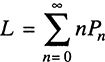
Starting with the balance equation for state 0, one finds that P1 = (λ/μ)P0. Adding the equation for state 0 to that of state 1 results in λP0 + μP2 + μP1 = λP1 + μP1 + λP0, which simplifies to μP2 = λP1. This means that P2 = (λ/μ)P1 and using the previous result that P1 = (λ/μ)P0, one finds that P2 = (λ/μ)2P0. In the same manner, by adding the simplified equation μP2 = λP)1 to the balance equation for state 2, one finds that λP1 + μP3 = μP2 = μP2 + λP1, which simplifies to μP3 = μP2. Note that this equation is identical to the balance equation for state 3, which then becomes redundant. P3 can now be expressed in P0 as follows: P3 = (λ/μ)P2 = (λ/μ)3P0. Using the expressions P1 = (λ/μ)P0, P2 = (λ/μ)2P0, and P3 = (λ/μ)3P0, together with the condition that P0 + P1 + P2 + P3 = 1, the following is obtained.
TABLE 6.1 Balance Equations for the Queuing Process at TravelCall


watch result in
Because it is known that λ = 9 and μ = 10, one can obtain P0 = 0.2908. Because P1 = (λ/μ)P0, P2 = (λ/μ)2P0, and P3 = ((λ/μ)3P0, one also has P1 = (9/10)P0 ≈ 0.2617, P2 ≈ (9/10)2P0 ≈ 0.2355, and P3 = (9/10)3P0 ≈ 0.2120.
These calculations predict that in steady state, the travel agent will be idle 29 percent of the time (P0). This also represents the probability that an arbitrary caller does not have to spend time in the queue before talking to an agent. At the same time, it is now known that 21 percent of the time the system is expected to be full (P3). This means that all new callers get a busy signal, resulting in losses for the agency. Moreover, the probability that a customer who calls in will be put on hold is P1 + P2 ≈ 0.2617 + 0.2355 ≈ 0.50.
Although the explicit costs involved have not been considered, it seems reasonable that TravelCall would like to explore the possibilities of allowing more calls to be put on hold; that is, to allow a longer queue. This way, they can increase the utilization of the travel agent and catch some customers who now take their business elsewhere. Another more drastic option to reduce the number of lost sales might be to hire one more travel agent.
The procedure for determining the stationary distribution of a general birth-and-death process with state-dependent arrival and service rates is analogous to the approach explained in Example 6.1. The balance equations are constructed in the same way, but their appearance is slightly different, as shown in Table 6.2. (See also the corresponding rate diagram in Figure 6.6.)
A complicating factor is that a large state space — one with many states to consider — means that it would be tedious to find a solution following the approach in Example 6.1. For example, to handle the cases of infinite queue lengths, some additional algebraic techniques are needed to obtain the necessary expressions. This is the motivation for studying the specialized models in Sections 6.4 through 6.7, where expressions are available for the steady-state probabilities and for certain important performance measures such as average number of customers in the system and queue, as well as the corresponding waiting times. Still, for smaller systems, the general approach offers more flexibility.
TABLE 6.2 Balance Equations for the General Birth-and-Death Process

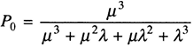
As previously mentioned, interesting performance measures for queuing processes are the average number of customers or jobs in the system (L) and in the queue (Lq), as well as the corresponding average waiting times (W and Wq). With the stationary probability distribution {Pn; n = 1, 2, 3, …} available, it is straightforward to obtain all these measures from the definition of expected value and Little’s law. (See Section 6.2.2 for the general expressions.) Next is an explanation of how to do this in the context of Travel Call Inc.
Example 6.2: Determining Average Performance Measures at TravelCall
In Example 6.1, the steady-state probability distribution was determined for zero, one, two, and three customers in the queuing system describing the operations at Travel Call. The probabilities were P0 = 0.2908, P1 = 0.2617, P2 = 0.2355, and P3 = 0.2120. Although interesting information, Travel Call also wants know what this means in terms of average performance measures.
- The expected number of customers in the system = L.
- The expected number of customers waiting in the queue = Lq.
- The expected time a customer spends in the system = W.
- The expected time a customer spends in the queue before being served = Wq.
Because the probabilities of having zero, one, two, and three customers in the system are known, to calculate L simply apply the definition of an expected value as follows.

To calculate Lq, proceed in a similar way but subtract the one customer that is being served in all those situations (states) where one or more customers are in the system. To clarify, when one customer is in the system, this customer is being served by the travel agent so the queue is empty. If two customers are in the system, n = 2, then one is being served by the travel agent and one is waiting in the queue. Finally, if three customers are in the system, then two of them are in the queue. The expected number of customers in the queue is obtained in the following way.
To determine the mean time spent in the system, W, and the mean time spent in the queue, Wq, use Little’s law as discussed in Section 6.2.2.

First determine the average arrival rate, which is not λ because when three customers are in the system, no more customers can be accommodated and the arrival rate for state 3 is effectively zero. For all other states, the arrival rate is λ. See Figure 6.7.

W and Wq can now be obtained from Little’s formula.

Note that W − Wq = 11.6 − 5.6 = 6 minutes, which is the expected service time, or 1/μ. With these average performance measures, Travel Call is in a better position to decide whether something needs to be done with respect to the system design. The waiting time of 5.6 minutes on the average might not seem long; however, for the customer waiting at the other end of the phone line, this might be perceived as a very long time, and it could lead to reneging (customer leaving the queue before being served; see Section 6.1.1).
Thus far, the examples have assumed that the service facility has a constant mean service rate. To illustrate a more general model, Example 6.3 extends Examples 6.1 and 6.2 to a situation with two travel agents and state-dependent mean service rates. By relating back to the results in Examples 6.1 and 6.2, this example also shows how these types of queuing models can be used for better-informed design decisions.
Example 6.3: TravelCall Inc. Revisited
Based on the queuing analysis performed on the existing process in Examples 6.1 and 6.2, the management of Travel Call is contemplating hiring a second travel agent. However, before proceeding they want to investigate the effects such a design change might have regarding the following.
- The fraction of time, or equivalently, the probability that the system is empty.
- The fraction of time that the system is full and potentially loses customers.
- The probability that acustomer gets to talk to a travel agent immediately.
- The probability that acustomer will be put on hold.
- The average performance measures L, Lq, W, and Wq.
The second travel agent is presumed to be just as efficient as the existing one, meaning the service time for the new agent is also exponentially distributed with the parameter μ = 10 customers per hour. The customer arrival rate is assumed unaffected; that is, Poisson distributed with mean rate λ = 9 customers per hour. Moreover, the travel agents work independently of each other and fully service one customer at a time. (In fact, Travel Call will encourage them to work from their homes and thereby reduce the overhead costs for office space, still using a common switchboard though.) As a result, the travel agency can be modeled as a queuing system with two parallel and identical servers. Recall from Section 6.1 that this means the mean service rate for the service facility is 2μ when both servers are busy and μ when only one server is busy. This observation is key in constructing the correct rate diagram shown in Figure 6.8. Starting in state 0, no customers are in the system so the service rate is zero and the arrival rate is λ. In state 1, one customer is in the system, and is currently being served by one of the travel agents at the service rate μ. The arrival rate is unaffected and equals λ. In state 2, two customers are in the system, each being serviced by a travel agent. As discussed previously, the service rate for the service facility with the two parallel agents is then 2 μ.The arrival rate is still λ. In state 3, three customers are in the system, one in the queue and two being serviced in parallel. The combined service rate for the two agents is, therefore, still 2μ. The arrival rate, on the other hand, is zero because the system is full and any new arrivals are turned away.

FIGURE 6.8 Rate Diagram for the Two Server Queuing Processat Travel Call

Based on the rate diagram, the balance equations can be formulated as in Table 6.3, assuring that for each state the expected rate in equals the expected rate out.
Solving the equation system in the same way as described in Example 6.1, one obtains P1, P2, and P3 expressed in P0: P1 (λ/μ)P0, P2 = (λ2/2/μ2)P0, P3= (λ3/4/μ3)P0. Using these expressions in conjunction with the condition that the steady-state probabilities must sum to 1; that is, the system must always be in one of the attainable states, P0 + P1 + P2 + P3 = 1, one gets the following.

Which result in

With λ = 9 and μ = 10, this means P0 ≈ (1/2.48725) ≈ 0.4021 and consequently P1 - (λ/μ)P0 = (0.9)P0 ≈ 0.3618, P2 = (λ2 /2/μ2)P0 = (0.92/2)P0 ≈ 0.1628, and P3 = (λ3/4/μ3)P0 = (0.93/4)P0 ≈ 0.0733. It can then be concluded that in the new design:
- The fraction of time that the system is empty = P0 ≈ 40 percent.
- The fraction of time that the system is full and potentially loses customers = P3 ≈ 7 percent.
- The probability that a customer gets to talk to a travel agent immediately = P0 + P1 ≈ 76 percent.
- The probability that a customer will be put on hold = P2 ≈ 16 percent.
With the steady-state probability distribution in place, the expected number of customers in the system and in the queue, L and Lq, respectively, can be determined. (In comparingthe expressions that follow with the general formulae, note that in the present case c = 2 and Pn = 0 for n > 3.)
![]() = (0)P0 + (1)P1 + (2)P2 + (3)P3 = 0.3618 + (2)0.1628 + (3)0.0733 = 0.9073 ≈ 0.91 customers
= (0)P0 + (1)P1 + (2)P2 + (3)P3 = 0.3618 + (2)0.1628 + (3)0.0733 = 0.9073 ≈ 0.91 customers
![]() = (2 − 2)P2 + (3 − 2)P3 = (1)0.0733 ≈ 0.07 customers
= (2 − 2)P2 + (3 − 2)P3 = (1)0.0733 ≈ 0.07 customers
TABLE 6.4 Comparison of the Process Performance When There Are Two Travel Agents at TraveiCalllnstead of One

The expected time in the system, W, and in the queue, Wq, can now be obtained from Little’s law.

Table 6.4 contrasts the results obtained for the system with two travel agents with those obtained for the current single-server system evaluated in Examples 6.1 and 6.2.
Hiring a second agent dramatically increases the customer service levels. For example, the probability that a customer will get immediate access to an agent goes up from 29 percent in the single-server system to 76 percent when two travel agents are working the phones. At the same time, the average waiting time on hold decreases from 5.6 minutes in the current single-server process to 0.5 minutes in the new design. Moreover, in terms of potentially lost sales, customers in the two-server system encounter a busy signal only 7 percent of the time compared to 21 percent in the single-server system.
This improved service comes at the expense of lower resource utilization, indicated by the fact that the fraction of time the system is empty goes up from 29 percent in the single-server system to 40 percent in the system with two agents. Hiring the second travel agent also increases the operational costs significantly. In order to make an informed decision whether to pursue the new design, these service costs must be quantified and compared against the expected revenue increase due to the improved customer service. Models dealing with these issues will be examined in Section 6.2.8.
Hiring a second agent is just one possibility for changing the process design. Another option is to allow customers to contact the travel agent via other channels, such as through a Web site or e-mail. In this way, the existing travel agent can work with these requests between phone calls. Most likely, it also will lead to fewer customers calling, implying shorter waiting times for telephone customers and a lower risk of encountering a busy signal. A further analysis of this option is beyond the scope of this example but illustrates the potential advantages of thinking about doing things in new ways. Another example of creative design ideas, which relates to the design principle of treating geographically dispersed resources as if they were centralized, as discussed in Section 3.6.2, is letting the travel agents work from their homes.
Examples 6.1 through 6.3 assume that customers who have the opportunity to enter the queue also will choose to join it. However, some customers, after realizing that they will have to wait before getting served, will choose to leave; in other words, they will balk. Balking can be modeled as state-dependent arrival rates using the fact that Poisson processes can be disaggregated into new Poisson processes, as seen in Section 6.2.1. Assume, for example, that customers calling Travel Call in Example 6.3 will hang up with probability β if they don’t get immediate access to a travel agent. This means that as soon as both travel agents are busy, the arrival process will be Poisson with mean arrival rate (1 − β )λ as opposed to a mean arrival rate of λ for the other states. Figure 6.9 shows the corresponding rate diagram. It might be hard to assess an accurate value of β because customers who hang up are not registered. Most likely, a market research effort would have to be launched to explore and better understand customer attitudes.

FIGURE 6.9 Rate Diagram for the Two Server Queuing Process at Travel Call if Customers Balk with Probability β, When They Do Not Get Immediate Access to a Travel Agent
Given the rate diagram in Figure 6.9, the model with balking can be analyzed using the same approach as in Examples 6.1 through 6.3.
The discussion on balking and state-dependent arrival rates concludes this investigation of the general birth-and-death process. Sections 6.2.4 through 6.2.7 focus on some important birth-and-death processes with specialized structures that are often used in queuing analysis. Their importance stems from their wide applicability and the expressions that make it straightforward to evaluate important performance measures quickly. Still, it is important to remember that all of these models are specialized birth-and-death processes that can be analyzed using the general approach explored in this section.
6.2.4 THE M/M/1 MODEL
The M/M/1 model is a special case of the general birth-and-death process described in Section 6.2.3. Because of its simplicity, it has found applications in a wide range of areas, and it is one of the most commonly used queuing models. It describes a queuing system with a single server, exponentially distributed service and interarrival times, constant arrival and service rates, an infinite calling population, and no restrictions on the queue length. More precisely, going back to the major elements of the basic queuing process, the model is based on the following assumptions.
- Calling population: Jobs arrive from such a large population that it can be considered infinite for modeling purposes. The jobs are independent of each other; that is, the arrival of one job does not influence the arrival of others. Also, the arrival of jobs is not influenced by the system (e.g., there are no appointments).
- Arrival process: The interarrival times are exponentially distributed with a constant parameter λ, independent of the number of customers in the system. In other words, the arrival process is Poisson with the mean rate λ, independent of the state of the system.
- Queue configuration: A single waiting line is used with no restrictions on length. The model does not consider balking or reneging.
- Queue discipline: The queue is managed using a FIFO rule.
- Service mechanism: The service facility consists of a single server, whose service times are exponentially distributed with a constant parameter μ, independent of the number of customers in the system. Consequently, the mean service rate is μ for all states of the system.
The M/M/1 process can be illustrated by the rate diagram in Figure 6.10. Recall from Section 6.2.3 that in this diagram, the states, that is the number of customers in the system, are depicted as numbered circles or nodes (node 0 indicates state 0 with zero customers in the system), and the transitions between these states are indicated by arrows or directed arcs. Furthermore, the rate at which the system moves from one state to the next is displayed in connection with each arc. As discussed previously, customers or jobs arrive to the system at the mean rate λ, independent of the number of customers currently in the system. Consequently, the rate at which the process moves from state n to state n + 1 is λ for all n = 0, 1, 2, … . Similarly, the mean service rate at which the server services customers is μ for all states where there is someone to serve; that is, allstates except state 0 when the system is empty and the service rate is zero. As a result, the rate at which the process moves from state n to n − 1 is μ for all n = 1, 2, … .
For the steady-state analysis of the M/M/1 model, the following notation, first introduced in Section 6.2.2, is used.
Pn = The probability of finding exactly n customers or jobs in the system, or equivalently, the probability that the system is in state n
λ = The mean arrival rate (the mean number of arrivals per time unit); the same for all system states
μ = The mean service rate (the mean number of service completions per time units in a busy server); constant for all relevant system states
ρ = λ/μ = utilization factor
L = The expected number of customers or jobs in the system including the queue and the service facility
Lq = The expected number of customers or jobs in the queue
W = The expected time customers or jobs spend in the system including waiting time in the queue and time spent in the service facility
Wq = The expected time customers or jobs spend waiting in the queue before they get served
A necessary and sufficient condition for the M/M/1 process to reach steady state — that is, for the existence of a steady-state probability distribution {Pn, n = 0, 1, 2, …} — is that the mean arrival rate λ is strictly less than the mean service rate μ, or equivalently ρ < 1. The analysis and expressions that will be explored in this section therefore assume that ρ < 1. If ρ ≥ 1, it means that the average demand for service exceeds the average service capacity and the queue will explode in size.

FIGURE 6.10 Rate Diagram for the M/M/1 Model
The steady-state operating characteristics of the M/M/1 system can be calculated from the following set of expressions. (The expressions can be derived using the general approach for analyzing birth-and-death processes in Section 6.2.3.)
Probability of zero jobs in the system:
Probability that the number of jobs in the system is exactly n:
MATHEMATICAL DERIVATION
Using the rate diagram in Figure 6.10, it is straightforward to construct the balance equations for the M/M/1 queue using the approach in Section 6.2.3. See also Table 6.2 with λn = λ and μn = μ for all n. From these equations, it follows that P1 = (λ/μ)P0 = ρP0, P2 = ρ2P0, … and consequently Pn = ρnP0.
To determine P0, invoke the condition ![]() which results in:
which results in: ![]()
Observing that ![]() is the sum of a geometric series for which it is known that
is the sum of a geometric series for which it is known that ![]() for any ρ < 1 we get P0 = 1 − ρ.
for any ρ < 1 we get P0 = 1 − ρ.
Probability that the number of jobs in the system is k or more:
Probability that the number of jobs in the system is at least one:
Because P(n ≥ 1) also represents the probability that the server is busy, it explains why ρ is known as the utilization factor for the server in this model.
MATHEMATICAL DERIVATION

where we use that ![]() for any ρ < 1
for any ρ < 1
Mean number of jobs in system
MATHEMATICAL DERIVATION

 for ρ < 1.
Mean time a job spends in the system:

MATHEMATICAL DERIVATION

Where we use P0 = 1 − ρ.
Mean time a job spends in the system:
Mean time a job spends in the queue:

MATHEMATICAL DERIVATION
The expressions follow directly from Little’s law, ρ = (μ/λ), and the aforementioned expressions for L and Lq.

Example 6.4 illustrates how the previous expressions can be used to analyze a business process that can be modeled as an M/M/1 system.
Example 6.4: Policy Requests at an Insurance Company
An insurance company receives an average of 40 requests for new auto policies per week. Through statistical analysis, the company has been able to determine that the time between two consecutive requests arriving to the process is approximately exponentially distributed. A single team handles the requests and is able to complete an average of 50 requests per week. The actual times to complete requests also are considered to follow an exponential distribution. The requests have no particular priority; therefore, they are handled on a first-come-first-served basis. It also can be assumed that requests are not withdrawn.
What is the probability that an arriving request must wait for processing? That is, what is the probability that the team will be busy working on a request when a new request arrives?
What is the probability that an arriving request does not have to wait? That is, what is the probability that the arriving request will find the team idle?
What is the expected number of requests in the process?
What is the expected number of requests in the queue?
What is the average time that a request spends in the process? In other words, what is the average cycle time?
(It is assumed that a week has 5 working days and that each day has 8 hours.)
What is the average waiting time?
From these calculations, it can be predicted that the team will be busy, in the long run, 80 percent of the time. Therefore, 80 percent of the time an arriving request will have to join the queue instead of receiving immediate attention. The average cycle time is estimated to be 4 hours, from which 3.2 hours are expected to be waiting time. This calculation reveals that only 20 percent of a request’s cycle time is spent in value-adding activities, and the other 80 percent consists of a non-value-adding waiting time.
Another operating characteristic that can be calculated is the probability that a given number of jobs are in the process (either waiting or being served) at any point in time. This calculation is performed using the equation for Pn, where n is the number of jobs in the process. Figure 6.11 shows a plot of the probability values associated with a range of n-values from 0 to 20.

Figure 6.11 shows that the probability of finding n jobs in the process significantly decreases for n ≥ 10. In fact, the exact value for the probability of finding 10 jobs or more in the process is P(n ≥ k) = pk ≈ (0.8)10 ≈ 0.1074. This means that the probability of finding fewer than 10 jobs in the process is almost 90 percent.
In some processes where space needs to be provided for jobs in the queue, the ability to estimate the probability of the number of jobs in the system is critical. For example, suppose that technical support for a popular piece of software is provided via a toll-free telephone number. The process designer needs to know the expected number of customers that typically would be put on hold to provide the necessary “space” in the telephone system. In the same way, it is important to estimate the waiting time that customers would experience with different levels of staffing.
6.2.5 THE M/M/C MODEL
The M/M/c model is a generalization of the M/M/1 model that allows for multiple parallel servers in the service facility. More precisely, the added feature is that the service facility can consist of c identical parallel servers each with a constant service rate, µ and exponentially distributed service times working independently of each other. Still, with exception for the server configuration, the assumptions defining the M/M/c model arethe same as for the M/M/1 model, implying that the M/M/c model also represents a birth-and-death process. Figure 6.12 describes the M/M/c process in terms of its rate diagram. Note that for state 1,2, … , c, all customers or jobs in the system will be under service and the queue will be empty. This means that these states will have 1,2, … , c independent servers working in parallel, each with the service rate µ. From property 3of the exponential distribution discussed in Section 6.2.1, it can be concluded that the service rates for the service facility in state 0,1, 2, … , c are 0, µ, 2µ, … , cµ, respectively. For states c + 1, c + 2, … , all c servers are busy and the service rate for the service facility is cµ, so the additional customers have to wait in the queue. The arrival rate is independent of the system state and equal to λ.

FIGURE 6.12 Probability of n Jobs In an M/M/1 System with ρ = 0.8
In order for the M/M/c model to reach steady state, the mean arrival rate λ must be less than the mean service rate when all c servers are busy, that is, cμ. Because the utilization factor of the service facility ρ is defined as ρ = (λ/cμ) (see Section 6.2.2), the following relationship must hold in order for the M/M/c queue to reach steady state.

In other words, the utilization of the service facility, ρ, must be less than 100 percent for the M/M/c system to reach steady state; otherwise, the queue will explode in size and grow infinitely large.
As with the M/M/1 process, a set of expressions can be identified for evaluating the operating characteristics of this system. See, for example, Hillier and Lieberman (2001). These equations can be derived from the approach used for analyzing the general birth-and-death process, but the algebra poses more of a challenge. Therefore, the mathematical derivations of the following expressions are omitted.
Probability of zero jobs in the system:

Probability that all servers are busy:

Probability of exactly n jobs or customers in the system:

Mean number of jobs in the system:

Mean number of jobs in the queue:

Note that if the steady-state criteria ρ < 1 is violated and ρ = 1, L and Lq will become infinite because their expressions include a division with zero.
Mean time a job spends in the system:

Mean time a job spends in the queue:
A useful observation is that if Lq is known, the expressions for Wq, W, and L can be found easily using Little’s law and the relationship W = Wq + (1 /µ) discussed in Section 6.2.2. The expressions are: Wq = (Lq/λ); W = Wq + (1/µ) and L = λW = λ(Wq + 1/µ) = Lq + λ/µ.
To illustrate how the above formulae can be used to analyze a queuing system with parallel servers, Example 6.5 extends Example 6.4 to a situation with two servers.
Example 6.5: Policy Requests at an Insurance Company Revisited
Suppose the insurance company in Example 6.4 contemplates hiring a second team. However, before making a decision, they want to investigate the effects this will have on several important operating characteristics. A realistic assumption is that the new team will be just as efficient as the existing team, and for modeling purposes they can be treated as parallel servers with identical service rates. Because the only difference from the situation described in Example 6.4 is that the new process will have two independent teams handling the arriving requests, the new process conforms to an M/M/c queuing model with c = 2.
Recall from Example 6.4 that λ = 40 requests per week and µ = 50. The new system has two parallel servers, so c = 2. The corresponding utilization factor for the service facility is then:
Also note that just as in Example 6.4, (λ/µ) = 0.8.
The first question posed by the insurance company concerns the probability that an arriving request must wait for processing. That is, what is the probability that both teams will be busy working on requests when a new request arrives?
To provide an answer, first calculate the probability of zero requests in the system. (Recall that n! = n(n − 1 )(n − 2)… (2)(1) where by definition 0! = 1).

Then for c = 2, P(n ≥ c) is calculated as follows:

A related question concerns the probability that an arriving request gets processed immediately. That is, what is the probability that the arriving request will find at least one team idle?

Note that this probability is the complement of the probability of finding two or more requests in the process. Mathematically, this means that P(n < 2) = 1 − P(n ≥ 2) ≈ 1 − 0.23 = 0.77.
An important operating characteristic is the average work-in-process (WIP), or equivalently: What is the expected number of requests in the process?

A related performance measure is the expected number of requests in the queue.
Finally, the time measures W and Wq need to be analyzed. The first question is about the average time that a request spends in the process. In other words, what is the average cycle time W?
(As before, assume that a week has 5 working days and that each day has 8 hours.)
Second, what is the average waiting time for a job before it is processed? That is, what is the value of Wq?
To summarize the results, the average utilization of the two teams is ρ = 40 percent. The average cycle time is estimated to be 57 minutes (i.e., 0.95 hours), of which only 9 minutes are expected to be waiting time. The cycle time reduction is significant when compared to the 4 hours achieved with a single server. This reduction translates into 84.2 percent (i.e., 48/57) of value-adding activity time and 15.8 percent (i.e., 9/57) of non-value-adding activity time in the two-server system. In the single-server system, only 20 percent of a request’s cycle time is spent in value-adding activities, and the other 80 percent consists of non-value-adding waiting time.
The decision about whether to increase the service capacity must be made based on the benefits associated with reducing non-value-adding time (in this case, waiting time) and the cost of achieving the reduction. Going from a one-server system to a configuration with two teams working in parallel reduces total expected cycle time from 4 hours to 0.95 hours. However, at the same time the utilization of the servers drops from 80 percent to 40 percent when the number of servers is increased. To assess this economic tradeoff, the operating characteristics need to be translated into monetary terms, as explored in Section 6.2.8.
Next, two generalizations of the M/M/c model will be considered: allowing limitations on the queue length and the size of the calling population.
6.2.6 THE M/M/c/K MODEL
The M/M/c/K model imposes the restriction that at most K customers can be in the M/M/c system at the same time. This means that the system is full when K customers are in it, and customers arriving during this time are rejected. This type of queuing model is applicable in situations when the queuing system has a limited capacity to harbor customers. Examples include a limitation on the number of beds in a hospital, the size of a switchboard at a call center, the size of the waiting room at a barbershop, the size of a car wash, a computer network, or a parking lot. The M/M/c/K model also addresses the balking behavior of customers who choose to go elsewhere if they arrive when K customers are already in the system.
Apart from the constraint of no more than K customers in the system, the M/M/c/K model is based on the same assumptions as the M/M/c model: a single queue, exponential service and interarrival times, FIFO queuing discipline, and c identical servers in parallel working independently from one another, each with a mean service rate of µ. The difference is that because no more than K customers are allowed in the system, the arrival rate is zero for states K, K + 1, K + 2, … , but is λ for states 0,1,2, … , K − l.This is illustrated in the rate diagram for the M/M/c/K model in Figure 6.13. It follows that the M/M/c/K model is a birth-and-death process with state-dependent service and interarrival rates.

The queuing models analyzed in Examples 6.1 through 6.3 fall into the class of M/M/c/K models.
An important observation is that the M/M/c/K queue is guaranteed to reach steady state even if ρ – (λ/cµ) ≥ l. This is so because the queue can never grow infinitely large. As a matter of fact, it can never be larger than K – c customers or jobs (or equivalently, the number of customers in the system cannot exceed K as shown in Figure 6.13). In this model, at most K servers can be busy at the same time. Therefore, without loss of generality, the following exposition assumes that c ≤ K
As in the case of M/M/1 and M/M/c models, a set of expressions exists for calculating important performance characteristics for the M/M/c/K model. Although the approach for analyzing general birth-and-death processes could be used, algebraically it can be tedious for large K values. Therefore, the following expressions can be used to characterize the performance of M/M/c/K systems. In addition to the assumption that c ≥ K, the expressions use that ρ = (λ/cµ).

FIGURE 6.13 Rate Diagram (or the M/M/c/K Model
Probability of zero jobs in the system:

Probability of exactly n jobs in the system:

Menan number of jobs in the queue:

Note that the expression for Lq is not valid for ρ = 1. However, this does not imply that steady state is never reached for ρ = 1. It is simply a result of how the expression is derived. The case of ρ = 1 can be handled separately, but this special case is not shown here.
Mean number of jobs or customers in the system:

Observe that the last two terms in the expression for L represent the expected number of jobs in the service facility. In other words, the expression corresponds to the sum of the average number of jobs in the queue and the average number of jobs in the service facility.
Applying Little’s law, it is easy to obtain the expected time spent in the system and in the queue. The average arrival rate in this case is:

Mean time a job or a customer spends in the system:

Mean time a job or a customer spends in the queue:

In Example 6.6 the travel agency TravelCall Inc. is used to illustrate how the M/M/c/K model works. Example 6.6 studies the same process as in Example 6.3, but the performance measures are now determined from the expressions of the M/M/c/K model instead of using the general approach investigated in Section 6.2.3. For convenience, the TravelCall process is described again.
Example 6.6: TravelCall Inc. Revisited: A Streamlined Approach
Recall from Example 6.1 that TravelCall Inc. is a small travel agency that services customers over the phone. The agency employs only one travel agent to answer incoming customer calls. However, management is contemplating hiring a second agent and wants to investigate how the system would perform with two agents. It is assumed that these two agents would work independently on separate customers, and that their service rates would be identical. The switchboard accommodates one call on hold in addition to the two routed to the travel agents. Customers who call when the switchboard is full will get a busy signal. Consequently, the maximum number of customers in the queuing system is three. The calls arrive to TravelCall according to a Poisson process with a mean rate of nine calls per hour, and the calls are answered in the order they arrive, so the queuing discipline is FIFO. On average, it takes a travel agent 6 minutes to service a customer, and the service time follows an exponential distribution. The travel agency wants to determine the probability of finding zero, one, two, or three customers in the system, as well as the average performance measures L, Lq, W, and Wq.
The queuing system at TravelCall fits the M/M/c/K model with c = 2 and K = 3, meaning a two-server system with at most K = 3 customers allowed in the system at the same time.Furthermore, the model can be described in terms of the rate diagram in Figure 6.14, which has the same structure as the rate diagram for the general M/M/c/K process in Figure 6.13.
As before, the first step in the numerical analysis is to decide on a time unit and to determine the mean arrival and service rates. All rates will be expressed in number of occurrences per hour. The mean arrival rate when no more than three customers are in the system is λ = nine calls per hour and zero otherwise (see Figure 6.14). Furthermore, the mean service rate for each of the two servers is µ = 60/6 = 10 calls per hour. This means that the utilization factor is ρ = λ/cµ = 9/((2)(10)) = 9/20 = 0.45.
First, the probability, P0, that the system is empty is determined.


FIGURE 6.14 Rate Diagram for the Two Server Queuing Processat TravelCall.
Then the probabilities P1, P2, and P3 can be obtained using:

These probability values are the same as those determined in Example 6.3.
The next step is to determine the expected number of customers in the queue, Lq, and in the system, L.

Finally, Little’s law is used to determine the mean time a customer spends in the system, W, and the mean time he or she spends in the queue, Wq.

A comparison with Example 6.3 verifies that the results are identical.
6.2.7 THE M/M/c/∞/N MODEL
The M/M/c/∞/N model is another generalization of the basic M/M/c model, which deals with the case of a finite calling population of N customers or jobs. Apart from this feature, the M/M/c/∞/N model is based on the same assumptions as the M/M/c model: a single queue, c independent, parallel and identical servers, exponentially distributed interarrival and service times, unlimited queue length, and a FIFO queuing discipline.
An important observation in understanding the M/M/c/∞/N model is that because the calling population is finite, each of the N customers or jobs must be either in the queuing system or outside , in the calling population. This implies that if n customers or jobs are in the system, meaning the queuing system is in state n , the remaining N – n customers or jobs are found in the calling population. When constructing the model, it is assumed that for each of the customers or jobs currently in the calling population, the time remaining until it arrives to the queuing system is independent and exponentially distributed with parameter λ. As a result, if n(n <= N) customers are in the queuing system, the arrivals at this system state occur according to a Poisson process with mean arrival rate (N – n) λ. (See Section 6.2.1.) To obtain this, let Tj be the time remaining until job j,j = 1,2, …, N – n in the calling population will arrive to the queue. The time remaining until the next arrival is then Tmin = min{T1, T2, … TN – n}.The conclusion follows because Tmin is exponentially distributed with parameter (N – n)λ. Assuming, as before, that the mean service ratefor each server is µ the M/M/c/∞/N model can be described by the rate diagram in Figure 6.15. Moreover, because the service and interarrival times are mutually independent and exponentially distributed, the M/M/c/∞/N model describes a birth-and-death process with state-dependent interarrival and service rates.

Figure 6.15 explicitly illustrates the fact that because only N jobs or customers are in the calling population, the maximum number of jobs or customers in the queuing system is N, which means that the maximum queue length is N – c. As a result, the M/M/c/∞/N model, like the M/M/c/K model, is guaranteed to reach a steady state even if ρ = ( λ/cµ) ≥ 1.
A common application area for the M/M/c/∞/N model is for analyzing machine maintenance or repair processes. These processes are characterized by c service technicians (or teams of service technicians) who are responsible for keeping N machines or service stations operational; that is, to repair them as soon as they break down. The jobs (or customers) in this queuing process are the machines or service stations. Those that are currently in operation are in the calling population, and those that are undergoing repair are in the queuing system. The service technicians or teams of technicians are the servers. For a maintenance process of this sort to be adequately described by an M/M/c/∞/N model, the time between breakdowns for each individual machine in operation needs to be exponentially distributed with a constant parameter, λ. Furthermore, the c service technicians (or service teams) should work independently from each other on separate machines all displaying exponentially distributed service times with the same service rate µ. Note that if n machines are undergoing repair, then N – n machines are in operation.
To analyze the performance of a given M/M/c/∞/N system, the general approach in Section 6.2.3 can be used; however, as with the M/M/c and M/M/c/K systems, the algebra can be somewhat tedious for larger systems. As an alternative, the following expressions have been derived to aid in the analysis. See, for example, Hillier and Lieberman (2001). It is assumed that c ≤ N.

FIGURE 6.15 Rate Diagram for the M/M/c/∞/N Model
Probability of zero jobs in the system:

Probability of exactly n jobs in the system:

Mean number of jobs or customers in the queue:
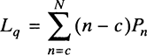
Note that this expression is simply the definition of Lq.
Mean number of jobs or customers in the system:
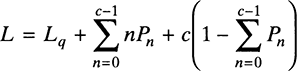
Observe that the last two terms in this expression for L represent the expected number of jobs in the service facility. Consequently, the expression simply adds the average number of jobs in the queue to the average number of jobs in the service facility.
To obtain the expected time spent in the system and in the queue, Little’s law can be used as discussed in Section 6.2.2. The average arrival rate in this case is:

Mean time a job or a customer spends in the system:
Mean time a job or a customer spends in the queue:
Remark The M/M/c/∞/N model is based on the assumption that the time an individual job or customer spends in the calling population outside the queuing system is exponentially distributed. However, it has been shown (see Bunday and Scraton, 1980) that the expressions for P0 and Pn (and consequently those for L, Lq, W and Wq) also hold in more general situations. More precisely, the time that a job or customer spends outside the system is allowed to have any probability distribution as long as this distribution is the same for each job or customer and the average time is 1/λ. Note that these situations fall outside the class of birth-and-death processes into a G/M/c/∞/N model.
Example 6.7 illustrates the analysis of an M/M/c/∞/N model in the context of a machine repair process as discussed previously.
Example 6.7: The Machine Repair Process at PaperCo Inc.
PaperCo Inc. is a manufacturer of fine paper. Its most important product is a special, environmentally friendly type of bleached paper used for laser printers and copiers. PaperCo has one production facility consisting of three large paper-milling machines. These machines are expensive and need to be kept operational to the largest extent possible. At the same time, their complexity makes them sensitive to malfunctions. Currently, PaperCo has one repair team on call 24 hours a day, 7 days a week. However, management is contemplating increasing this to two teams and would like a performance analysis of this double-team scenario. They already know the performance of the current process with one team. Each team is configured so that all competencies needed are available within the team, and having two teams working on the same machine provides no advantages. Therefore, it can be assumed that the two teams work independently from one another on different machines. Furthermore, their service times are assumed to be identical and exponentially distributed with a mean of 4 hours. Empirical data show that the time between malfunctions in each of the three machines when they are operating is exponential with a mean of 8 hours. The machines are equally important, so broken-down machines are serviced in a FIFO manner.
PaperCo wants to know the steady-state probabilities that zero, one, two, or three machines are nonoperational. They also want to determine the average time before a machine that breaks down is operational again, as well as how long on average a broken machine has to wait before a service team starts to work on the problem.
The first step in analyzing this problem is to recognize that the PaperCo repair process can be modeled as an M/M/c/∞/N system with c = 2 servers (the service teams) and N = 3 jobs in the calling population (the machines). Furthermore, the mean service rate for each of the two teams is µ = 1/4 = 0.25 jobs per hour, and the failure rate for each machine in operation is λ = 1/8 = 0.125 machines per hour. The rate diagram for the repair process is depicted in Figure 6.16. (See also Figure 6.15 for the general structure.) It should be noted that this problem can be analyzed using the general approach for birth-and-death processes discussed in Section 6.2.3, although a different method is used here.
Using the expressions given previously, one can determine the steady-state probabilities {Pn, n = 0,1,2,3} of zero, one, two, and three machines malfunctioning. Note that N = 3, c = 2, λ = 0.125, µ = 0.25, and (λ/µ) = 0.5.

FIGURE 6.16 Rate Diagram for the M/M/2/∞/3 Model Describing the Machine Repair Process at PaperCo
Probability of zero jobs in the system:

Probability of exactly n jobs in the system:

Mean number of jobs or customers in the queue:

Mean number of jobs or customers in the system:

= 1.0363 = 1.04 machine
Little’s law can be used to determine the expected downtime for a broken machine, W, and the expected time a broken machine has to wait for a service team, Wq.

Consequently, with two service teams all machines are operational 29 percent of the time, two out of three are working 44 percent of the time, two machines are down 22 percent of the time, and 5 percent of the time all three machines are standing still. Moreover, it takes 4 hours and 13 minutes on average from the moment a machine breaks down until it is up and running again, of which 13 minutes is waiting time before a team is available.
It seems that PaperCo needs to do something about this process. Even with two teams, a significant amount of costly downtime is occurring.
6.2.8 QUEUING THEORY AND PROCESS DESIGN
The analytical queuing models studied in Sections 6.2.3 through 6.2.7 have proven useful in analyzing the steady-state behavior of various queuing systems. The analysis focuses on the probability distribution for the number of customers in the queuing system and on the average performance measures, such as the mean queue length and the mean time customers spend in the queue and in the queuing system as a whole. Examples also have been provided of how this type of information can help the process designer better understand the impact that capacity-related decisions have on service to the customers. However, as discussed in the introduction to this chapter, an optimal design decision involves an economic trade-off between the cost of additional capacity and the cost of poor service in terms of long delays. This section explores these issues further, particularly by investigating how waiting costs (or shortage costs) can be used to translate the service performance into monetary terms. Challenges related with appropriately quantifying waiting costs also will be discussed. First, however, the decisions facing the process designer need to be examined.
When designing basic queuing systems such as those in Sections 6.2.3 through 6.2.7 — single-queue, parallel-server systems — two design parameters are usually under the decision maker’s control.
- The number of parallel servers in the service facility; for example, the number of physicians at a hospital ward, the number of checkout stations in a grocery store, or the number of operators in a call center.
- The service time or speed of individual servers; for example, size and thereby the service time of a repair team, the type of materials handling system (conveyor belts, forklift trucks, and so on) in a production facility, or the speed of an airplane transporting people.
In the context of the models in Section 6.2.3 through 6.2.7, these decisions involve determining c, the number of parallel and identical servers, and µ, the service rate for an individual server (assuming that the service time for individual servers is state independent). Another design parameter that might be under the decision maker’s control is K, the maximum number of customers in the system (or equivalently K − c as the maximum queue length). This could involve decisions regarding the number of calls that can be placed on hold at a call center, the size of the waiting area at a restaurant, the number of beds in a hospital, and so on. The effect of increasing K is that more customers fit into the system and fewer customers are denied service, but at the same time the waiting time for those in the system tends to increase. Translating these effects into monetary terms typically requires a somewhat more complex waiting cost structure than when considering changes only in c and µ. The following analysis assumes that K = ∞ and focuses on design changes in c and µ, meaning the focus is on designing M/M/c systems.
In addition to the design parameters, c and µ, which relate to the queuing system’s available capacity, the process design team sometimes is in a position to affect the demand for capacity through the arrival process. This could involve demand-management initiatives to reduce the variability in the demand pattern, making the arrival process more stable. Note, however, that under the assumption of exponentially distributed arrival times, it is not possible to reduce the demand variability without changing the mean demand. Consequently, the effects of demand management initiatives cannot be properly analyzed using the M/M/c models that have been introduced.
Given the available design parameters, the design team must decide how to set these parameters, meaning the amount and type of capacity to acquire in order to satisfy the customers’ service requirements. A fundamental design issue is therefore to quantify these service requirements. The two standard approaches are to specify an acceptable service level or to specify a waiting cost (or shortage cost).
For the service level approach, the decision problem is to minimize the capacity-related costs under the service level constraint; that is, to determine c, µ, and if applicable K, to minimize the expected cost of operating the queuing system given that the service level is met. Different ways of measuring the service level exist, such as the average waiting time, the percentage of customers receiving service immediately, or the percentage of customers waiting less than, say, 5 minutes.
The focus in this section is on the waiting cost approach. In this case, the corresponding decision problem is to determine c or µ to minimize the total cost of waiting and operating the queuing system. To investigate this further, some additional notation needs to be introduced.
WC = Expected waiting cost per time unit for the queuing system
SC = Expected service cost per time unit for operating the queuing system
TC = Expected total cost per time unit for the queuing system = SC + WC
Cw = Waiting cost rate = waiting cost per customer and time unit
Cs(µ) = Service cost per time unit for an individual server with service rate µ
It is worth noting that although a constant waiting cost rate, Cw, is assumed, it is straightforward to extend the analysis to state-dependent waiting cost rates, see, for example, Hillier and Lieberman (2001).
The decision problem can be stated as:
The corresponding cost functions, TC, SC and WC are illustrated in Figure 6.17.
Determining WC
In order to determine an expression for the expected waiting cost per time unit for the system, WC, note that if n customers are in the system, the waiting cost per time unit is Cwn. From the definition of expected value and the steady-state probability distribution for finding n customers in the system, an expression for WC can be found.


The expected waiting cost per time unit for the queuing system is obtained by multiplying the waiting cost per customer and per time unit with the expected number of customers in the system. This expression assumes that every customer in the queuing system incurs the same waiting cost whether the customer is waiting in the queue or is in the service facility. In cases where only the customers in the queue incur waiting costs, the expression for WC is:
If not otherwise specified, we will assume that the waiting costs are based on the number of customers in the system and not just those in the queue.
Determining SC
The expected service cost per unit of time for the system depends on the number of servers, c, and the speed of these servers. When all c servers are identical with service rates µ, the expected service cost can be expressed as follows.
A Decision Model for Designing Queuing Systems
Based on the expressions for WC and SC, a decision model for determining the values of the design parameters c and µ can be formulated as follows. The objective is to minimize the total costs per time unit for the entire queuing system.
Examples 6.8 and 6.9 illustrate how the process design team can use this general decision model for optimizing the performance of queuing systems.
Example 6.8: Process Design at CopyCo Inc.—The Option of a Second Machine
CopyCo is a small print shop located near a large university campus. Currently, all jobs involving paper-to-paper copies are carried out on one copy machine. For some time, CopyCo has experienced backlog problems with jobs submitted to the paper-to-paper copier. Management is worried that the long waiting times might be detrimental to future sales, so they are contemplating the acquisition of a second identical copy machine. The current machine is leased at a cost of $50 per day. Other costs for operating the machine, such as labor and electricity, amount to $150 per day. The second copier also would be leased, and it is estimated that it would accrue the same costs as the existing one—$200 per day. Empirically, it has been shown that the service and interarrival times are exponentially distributed. Furthermore, on average, CopyCo receives 95 jobs per day involving paper-to-paper copying, and the mean service time on the current machine is 6 minutes. CopyCo is open 10 hours per day, and the number of jobs that can be in the store at the same time is subject to no immediate space restrictions. The hourly waiting cost per customer is estimated to $5. Management wants to design the paper-to-paper copying process to minimize the total expected costs while considering the option of acquiring a second machine.
First, a suitable queuing model needs to be selected for this situation. It is known that the service and interarrival times are exponentially distributed, and that no restrictions are placed on the queue length. In the case of a single copier, the queuing process at CopyCo fits an M/M/1 model. In the case of two identical copiers working in parallel, the appropriate model is an M/M/2 model.
Because the objective is to find the design alternative that minimizes the total expected costs, an appropriate decision model is:
The only decision variable is the number of servers, c = 1 or 2. The service rate µ for each individual server is fixed.
The known cost, demand, and service information is
λ = 95 jobs per day = 95/10 = 9.5 jobs per hour,
µ = 60/6 = 10 jobs per hour,
Cs(µ) = $200 per day = 200/10 = $20 per hour,
Cw = $5 per customer and hour.
All parameters should be expressed in the same time units, and in this case hours have been chosen.
The only unknown values in this decision model are the expected number of jobs in the system for the single- and double-copier alternatives. Let L1 be the expected number of jobs in the M/M/1 system and L2 be the expected number of josbs in the M/M/2 system. Using the formulae from Sections 6.2.4 and 6.2.5 and the decision model, one gets:
M/M/1 system:

M/M/2 system:

Because the expected total cost is considerably lower with a second copy machine in place (TC2 < TC1), it is recommended that the CopyCo management team choose this alternative. This recommendation is made despite the fact that the service costs of operating the two copiers are twice as high as when only one copier is used.
Example 6.9: Process Design at CopyCo Inc.—The Option of a Single Faster Machine
As the management team at CopyCo contacted the leasing company to sign up for a second machine, the sales person informed them about another alternative. A brand new model of their old copier just came on the market. The new model is twice as fast as the old one, which for CopyCo would mean an estimated average service time of 3 minutes. The service times are assumed exponential, and the jobs arriving to the print shop are the same as before. The cost to lease this new model is $150 per day. Operating the new model efficiently will require additional personnel and more electricity, rendering an estimated operating cost of about $250 per day. Consequently, the total service cost of operating the new machine is $400 per day, which is the same as the cost of operating two of the old machines. The question is whether leasing one fast machine is better than leasing two slower copiers.
Because service and interarrival times are exponential and the queue length has no restrictions, the new alternative with one fast copier can be modeled as an M/M/1 queue.
From Example 6.8, it is known that
λ = 95 jobs per day = 95/10 = 9.5 jobs per hour
Cw = $5 per customer and hour
From the information about the new model of the copy machine, it is known that:
µnew = 60/3 = 20 jobs per hour
Cs(µnew)= $250 + $150 per day = 400/10 = $40 per hour
Because the objective is to find the design alternative that minimizes the total expected costs, an appropriate decision model is:
The decision variables in this case are the number of servers, c = 1,2, and their individual speed, µ = 10 or 20. However, only two alternatives are being compared: the alternative with two copiers of the old model—c = 2 and µ = 10 jobs per hour, and the alternative with one copier of the new model—c = 1 and µ = 20 jobs per hour. Furthermore, for the alternative with two copiers of the old model, the expected cost has already been determined in Example 6.8, TC2 = $46.15 per hour.
For the new alternative with one fast copier, the costs are obtained as follows:
M/M/1 system:
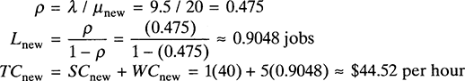
The cost comparison indicates that the alternative with one fast copier of the new model is preferable to the option of leasing two copiers of the old model ($44.52 < $46.15).
Remark. The conclusion in Example 6.9 is a consequence of a more general result regarding single- and multiple-server facilities with the same mean capacity. It can be shown that a queuing system with one fast server with service rate equal to cµ will always render shorter expected waiting times and fewer customers in the system than a service facility with c parallel servers, each with a service rate of µ. This also implies that the expected total cost TC is lower for the single-server system as long as the service cost SC is such that Cs(cµ) ≤ cCs(µ).
Thus far, it has been assumed that a relevant waiting cost rate Cw is readily available. Unfortunately, this is not always the case. In fact, finding an appropriate waiting cost rate is often a major challenge in the practical application of decision models based on waiting costs.
Because of the wide variety of queuing situations, there exists no single procedure for estimating the customers’ waiting cost rates or waiting cost functions. In fact, the entire waiting cost concept is situation dependent. For example, the waiting costs for long delays at an emergency room are very different from those experienced by customers in a supermarket. Essentially, the waiting cost rate should reflect the monetary impact that a delay of a single customer or job has on the organization where the queuing system in question resides. This implies that first, it is necessary to understand the consequences of time delays for the customers, and to understand customer requirements and behavior. Second, these consequences must be translated into monetary effects for the queuing system or the organization to which it belongs. This has to be done on a case-by-case basis. However, in broad terms, one can distinguish between situations in which the customers are external to the organization and ones in which they are internal. Furthermore, there is typically a difference between profit-maximizing organizations and nonprofit organizations.
In the case of external customers arriving to profit-maximizing organizations, the waiting costs are related primarily to lost profits and bad reputation affecting future sales. For example, long lines at a grocery store might discourage a customer from coming back or from entering the store in the first place. For nonprofit organizations, on the other hand, the waiting costs are typically related to future social costs. In order to estimate these costs, it is necessary to understand how waiting affects the individual customers and society as a whole. For example, what is the cost to society of having long waiting times at an emergency room? Social costs and costs related to lost profits can be hard to quantify in monetary terms. In some cases, it might be easier to estimate an acceptable service level and use the service level approach. Again, in other cases, the costs associated with delays and waiting might be easier to identify. Consider, for example, the drug approval process of a pharmaceutical company, which has a cost associated with its cycle time. If the process requires 1 year to be completed and 80 percent of this time is due to delays, then the cost of waiting is 9.6 months of lost sales. In this case, loss of market share due to late market introduction also should be added to the lost sales cost.
In situations where the arriving customers are internal to the organization where the queuing system resides, it is usually somewhat easier to estimate the waiting costs. The customers (or jobs) in these cases are typically machines or employees of the organization. Therefore, it is often possible to identify the immediate consequences associated with having these customers idle. The main component of the waiting costs associated with this idleness is, in most cases, the lost profit due to the reduced productivity.
Estimating waiting costs is often a challenging task based on customer requirements and the consequences of poor service. However, as discussed in Chapters 1 through 3, gaining an understanding of the customer requirements is at the core of effective business process design.
6.3 Introduction to Simulation
Section 6.2 explored how analytical queuing models offer powerful means for understanding and evaluating queuing processes. However, the use of these analytical models is somewhat restricted by their underlying assumptions. The limitations pertain to the structure of the queuing system, the way variability can be incorporated into the models, and the focus on steady-state analysis. Because many business processes are cross functional and characterized by complex structures and variability patterns, a more flexible modeling tool is needed. Simulation offers this flexibility and represents a powerful approach for analysis and quantitative evaluation of business processes.
In general, to simulate means to mimic reality in some way. Simulation can be done, for example, through physical models such as wind tunnels, simulators where pilots or astronauts train by interacting with a computer in a virtual or artificial reality, or through computer-based models for evaluation of a given technical system or process design. In the latter case, simulation software is used to create a computer model that mimics the behavior of the real-world process.
The rapid development of computer hardware and software in recent years has made computer simulation an effective tool for process modeling and an attractive technique for predicting the performance of alternative process designs. It also helps in optimizing their efficiency. Simulation is useful in this context because business process design is a decision-making problem for which the following is true.
- Developing analytical mathematical models in many cases might be too difficult or perhaps even impossible.
- The performance of a process design typically depends heavily on the ability to cope with variability in interarrival and processing times (implying a need for a modeling tool that can incorporate several random variables).
- The dynamics are often extremely complex.
- The behavior over a period of time must be observed to validate the design.
- The ability to show an animation of the operation is often an important way to stimulate the creativity of the design teams.
Despite its many virtues, simulation is sometimes met by skepticism from practitioners and managers. Much of the reluctance toward using simulation stems from the misconception that simulation is extremely costly and time-consuming. This is despite the many success stories showing that the savings from using simulation to improve process designs has far exceeded its costs. (See Examples 6.10 and 6.11.) In fact, with the advanced modeling tools that are currently available, the model development and experimentation phase might take only a few days or weeks, representing only a small fraction of the overall project development time (Harrell and Tumay, 1995). One of the most resource-consuming efforts that goes into building a valid simulation model is understanding how the process operates. However, as discussed in Chapter 3, this process understanding is a necessity for achieving an effective process design and must be done whether or not simulation is used. Savings from the use of simulation are well documented, as illustrated in Examples 6.10 and 6.11.
Example 6.10: Layout and WIP Investments
A Fortune 500 company used simulation for the design of a facility for producing and sorting subassembled components in preparation for the final assembly of a number of different metal products. One of the decisions involved determining the number of containers required to store the subassembled components. It initially was estimated that 3,000 containers were required. However, after a simulation study, it was found that throughput was not significantly affected when the number of containers varied from 2,250 to 3,000. By purchasing 2,250 containers instead of 3,000, savings of $528,375 was expected in the first year, with annual savings there-after of at least $200,000 from floor space (Law and McComas, 1988).
Example 6.11: Capacity Expansion in Connection with Facility Relocation
When a company decided to relocate to a new facility and expand its production capacity, it needed to analyze the impacts of changes in future demand. The relocation also provided the company with an opportunity to analyze its current production process and to seek improvements before increasing its capacity. Process simulation was used for capacity analysis and process improvement. Outputs from the process simulation were the primary inputs in determining the equipment and work-in-process inventory. The expansion alternatives from the process simulation identified the type and number of each piece of equipment needed to meet future capacity requirements. The queue lengths (average and maximum) were used to estimate the work-in-process inventory that needed to be accommodated at the new facility. Therefore, the facility layout design was fashioned along the recommended feasible alternatives and using other outputs from the process simulation, given the prescribed space constraints. The suggested layout design generated a throughput that exceeded the target production goal by 50 percent (Eneyo and Pannirselvam, 1999).
6.3.1 SIMULATION MODELS
Simulation models in general and computer-based models in particular can be classified in three different ways according to their attributes.
- Static or dynamic.
- Deterministic or stochastic.
- Discrete or continuous.
A static model is used when time does not play a role in the actual system. For example, a model of a bridge does not depend on time. A deterministic model is such that the outputs are fully determined after the inputs are known. Take a computer model for calculating the water pressure of a pipe network as an example. The pressure is known once the designer selects the pipe diameters for all the pipe segments. A discrete model considers that individual units (i.e., the transient entities of the system) are important. Most manufacturing, service, and business processes are discrete. Business processes in general are represented as computer-based dynamic, stochastic, and discrete simulation models.
A computer-based simulation model is an abstraction of the actual business process, represented in the computer as a network of connected activities and buffers (or equivalently, a network of basic queuing systems) through which jobs or customers flow. To provide a correct representation of the process, the model also must capture the resources and various inputs needed to perform the activities.
Because process modeling is only one application area for simulation modeling, a more general terminology for describing a simulation model is to refer to it as an abstraction of a system rather than a process. Conceptually, a system is defined as a collection of entities that interact with a common purpose according to sets of laws and policies. Entities are either transient or resident. In the process terminology defined in Chapter 1, transient entities are the jobs that flow through the system, and the resident entities are the buffers, workstations, and resources that make up the process network. Laws are not under the process designer’s control. Laws generally are represented by parameters. Sensitivity analysis is the experimentation used to determine the effect of changes in parameter values. Policies, on the other hand, are under the designer’s control. A policy typically is implemented by changing input factors. Design is the experimentation used to determine the effect of changes in input factors and system structure.
Example 6.12: An Order-Fulfillment Process
Consider an order-fulfillment process in which customers call a toll-free number to place an order. In this process, the orders are transient entities, and the sales representatives answering phone calls are resident entities. The arrival pattern of phone calls is a law, because it is beyond the process designer’s immediate control. The number of sales representatives can be controlled; therefore, it is considered a policy. In a simulation model of this process, the number of sales representatives can be expressed as an input factor so the analyst is able to experiment with different values, meaning that a sensitivity analysis can be carried out and the performance of the process can be tested (as measured, for example, by the cycle time).
In process design, models are used to study the behavior of a process. A process can be modeled symbolically, analytically, or with simulation. Symbolic models (or graphical tools) were introduced in Chapter 4. These models include process activity charts, process diagrams, and flowcharts. Symbolic models are quick and easy to develop, and are easily understood by others. The main disadvantage of symbolic models is that they fail to capture the dynamics of the process. Various analytical models have been investigated in Chapters 4 through 6. Deterministic models were introduced in Chapters 4 and 5, and stochastic models were introduced in Section 6.2. If their underlying assumptions were valid for a system under study, these models would be a convenient way to evaluate quantitatively different process designs. The main disadvantage is that these underlying assumptions are often restrictive. Furthermore, because these tools offer no obvious graphical representation, they might appear abstract to the process designer.
Modern simulation software in a sense combines the descriptive strength of the symbolic models with the quantitative strength of the analytical models. It offers graphical representation of the model through graphical interfaces, as well as graphical illustration of the system dynamics through plots of output data and animation of process operations. At the same time, it enables estimation of quantitative performance measures through statistical analysis of output data. The main disadvantage of simulation is the time spent learning how to use the simulation software and how to interpret the results.
To summarize, the following are some of the main attributes that make simulation powerful.
- Simulation, like analytical modeling, provides a quantitative measure of performance (e.g., resource utilization or average waiting time).
- Simulation, unlike analytical and symbolic models, is able to take into consideration any kind of complex system variation and statistical interdependencies.
- Simulation is capable of uncovering inefficiencies that usually go undetected until the system is in operation.
An interesting distinction between a simulation model and an optimization model is that simulation is a tool for evaluating a given design, and an optimization model is a tool used to search for an optimal solution to a decision problem. That is, a simulation model is by nature descriptive, and an optimization model is by nature prescriptive because it provides an optimal solution prescribing a course of action to the user.
Until recently, simulation software packages could be used only as what-if tools. This means that given a simulation model, the designer would experiment with alternative designs and operating strategies in order to measure system performance. Consequently, in such an environment, the model becomes an experimental tool that is used to find an effective design.
However, modern simulation software packages merge optimization technology with simulation. The optimization consists of an automated search for the best values (near-optimal values) of input factors (the decision variables). This valuable tool allows designers to identify critical input factors that the optimization engine can manipulate to search for the best values. The best values depend on the measure of performance that is obtained after one or several executions of the simulation model. The notion of optimizing simulations will be expanded in Chapter 10.
6.3.2 DISCRETE EVENT SIMULATION
Business processes usually are modeled as computer-based, dynamic, stochastic, and discrete simulation models. The most common way to represent these models in the computer is using discrete-event simulation. In simple terms, discrete-event simulation describes how a system with discrete flow units or jobs evolves over time. Technically, this means that the computer tracks how and when state variables such as queue lengths and resource availabilities change over time. The state-variables change as a result of an event (or discrete event) occurring in the system. A characteristic is that discrete-event models focus only on the time instances when these discrete events occur. This feature allows for significant time compression because it makes it possible to skip through all time segments between events when the state of the system remains unchanged. Therefore, in a short period of time, the computer can simulate a large number of events corresponding to a long real-time span.
To illustrate the mechanics of a discrete-event simulation model, consider an information desk with a single server. Assume that the objective of the simulation is to estimate the average delay of a customer. The simulation then must have the following state variables.
- Status of the server (busy or idle).
- Number of customers in the queue.
- Time of arrival of each person in the queue.
As the simulation runs, two events can change the value of these state variables: the arrival of a customer or the completion of service.
The arrival of a customer either changes the status of the server from idle to busy or increases the number of customers in the queue. The completion of service, on the other hand, either changes the status of the server from busy to idle or decreases the number of customers in the queue.
Because the state variables change only when an event occurs, a discrete-event simulation model examines the dynamics of the system from one event to the next. That is, the simulation moves the “simulation clock” from one event to the next and considers that the system does not change in any way between two consecutive events. For example, if a single customer is waiting in line at a grocery store and the next event is the completion of service of the customer who is currently paying for his groceries, then discrete-event simulation does not keep track of how the customer in the line spends her waiting time. In other words, the simulation keeps track of the time when each event occurs but assumes that nothing happens during the elapsed time between two consecutive events.
Figure 6.18 summarizes the steps associated with a discrete-event simulation. The simulation starts with initializing the current state of the system and an event list. The initial state of the system, for example, might include some jobs in several queues as specified by the analyst. It also could specify, for instance, the availability of some resources in the process. The most common initial state is to consider that no jobs are in the process and that all resources are currently available and ready. The event list indicates the time when the next event will occur. For example, the event list initially might include the time of the first arrival to the process. Other events might be scheduled initially, as specified by the analyst.
Once the initialization step is completed, the clock is advanced to the next event in the event list. The next event is then executed. Three activities are triggered by the execution of an event. First, the current state of the system must be changed. For example, the executed event might be a job arriving to the process. If all the servers are busy, then the state change consists of adding the arriving job to a queue. Other state changes might require deleting a job from a queue or making a server busy.

The execution of an event might cause the cancellation of other events. For example, if the executed event consists of a machine breakdown, then this event forces the cancellation of the processing of jobs that are waiting for the machine. Finally, the execution of an event may cause the scheduling of future events. For example, if a job arrives and is added to a queue, a future event is also added to the event list indicating the time that the job will start processing.
When an event is executed, the event is removed from the event list. Then the termination criterion is checked. If the criterion indicates that the end of the simulation has been reached, then raw data along with summary statistics are made available to the analyst. On the other hand, if the termination criterion indicates that the simulation has not finished (for example, because more events remain in the event list), then the clock is advanced to the time of the next event.
Example 6.13: Discrete-Events and Simulation Time Line in a Single-Server Process
A single-server queuing process can be represented with a time line on which the time of each event is marked. Assume the following notation.
- tj = Arrival time of the jth job,
- Aj = tj − tj−1 = Time between the arival of job j − 1 j
- Sj = Service time for job j
- Dj = Delay time for job j
- cj = tj + Dj + Sj = Compatation time for job j
- ei = Time of occurrence of event i
Figure 6.19 shows a graphical representation of the events in a single-server process. This example has six events, starting with event 0 and finishing with event 5.

Event 0, e0, is the initialization of the simulation. Event 1, e1, is the arrival of the first job, with arrival time equal to t1. The arrival of the second job occurs at time t2. Because c1 > t2, the second job is going to experience a delay. The delay D2 is equal to the difference between c1 and t2 (D2 = c1 − t2).
In Figure 6.19, the completion time for job 1 is calculated as c1 = t1 + S1, because this job does not experience any delay. The last event in this figure, labeled e5, is the completion time for job 2. In this case, the calculation of the completion time c2 includes the waiting time D2 (c2 = t2 + D2 + S2).
6.3.3 SPREADSHEET SIMULATION OF A SINGLE-SERVER PROCESS
It is possible to simulate a single-server process using an electronic spreadsheet program such as Microsoft Excel. The spreadsheet model must be capable of handling the following events.
- A job arrives.
- A job waits to be processed if the server is busy.
- A job is processed.
- A job leaves the system.
Next, a spreadsheet model will be created with the goal of estimating average waiting time and the percentage of time that the server is busy (the server utilization). To calculate waiting times, the arrival time of each job and its completion time must be known. To calculate idle time, one must know the time when processing starts for the current job and the completion time of the previous job. The following definitions are needed in addition to the variables defined in Example 6.13.
bj = Time when processing begins for job j
Ij = Idle time between job j and job j − 1
It is assumed that for each job, the interarrival time Aj and its service time Sj can be generated using a random generation function. Furthermore, it is assumed that the model being simulated is M/M/1. The interarrival and service times can be generated with the Excel functions RAND() and LN() and the following expressions.

In these expressions, µ is the mean arrival rate, and λ is the mean service rate. The Excel formula RAND() generates a random number between 0 and 1. The natural logarithm of the random number is found to transform this number into an exponentially distributed value. The transformation to an exponential distribution is completed when the value is divided by the appropriate mean rate and the negative sign is applied. (See Section 9.4 of Chapter 9 for a detailed explanation of how to generate exponentially distributed random numbers using this transformation.) The following relationships can be established based on the interarrival and service values.
Arrival time of the first job: t1 = A1
Arrival time of job j, for j > 1: t1 = A1 + tj-1
Starting time of the first job: b1 = t1
Starting time of job j, for j > 1: b1 = max(tj, Cj−1)
Delay time for job j: Dj = bj − tj
Idle time associated with the first job: I1 = t1
Idle time associated with job j, for j > 1: Ij = bj − cj − 1
Figure 6.20 shows a spreadsheet simulation of the M/M/1 model of Example 6.4. Recall that in this process, the arrival rate is 40 requests per week (λ = 40) and the service rateis 50 requests per week (µ = 50).
The spreadsheet simulation in Figure 6.20 uses the mean arrival rate and the mean service rate to generate interarrival times (D column) and service times (F column), respectively. The model simulates 200 requests and estimates the average waiting time and the server utilization. Note that the true average waiting time in steady state, as calculated using the analytical model, is 3.2 hours. The simulation of 200 requests shown in Figure 6.20 resulted in an estimated value of 3.621 hours. The average waiting time estimate by the simulation model approaches the analytical value as more requests are simulated; that is, as more rows are added to the spreadsheet.
The spreadsheet simulation also estimates the utilization of the server. The estimated value in the simulation shown in Figure 6.20 is 81.4 percent, which is close to the true steady-state value of 80 percent found with the analytical model. This estimate also improves when more requests are added to the simulation. The formulas needed to create the simulation model are shown in Table 6.5.
Table 6.5 shows the formulas for the first request (row 8) and the second request (row 9). All the other requests are modeled after the formulas in row 9. In order to calculate the statistics of interest (i.e., the estimated average waiting time and the estimated utilization), the following formulas are used in cells 13 and 14, respectively.
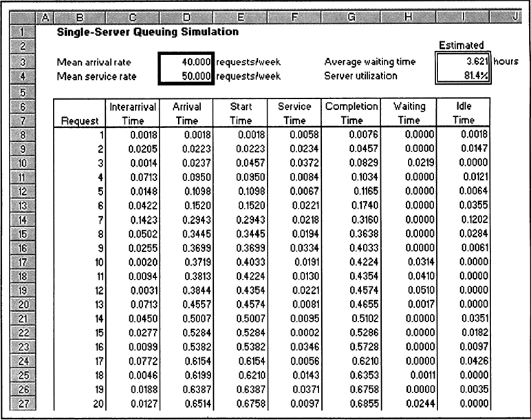
TABLE 6.5 Formulas for Spreadsheet Simulation

The average waiting time is multiplied by 40 to convert it from weeks to hours. The estimated utilization is based on the percentage of idle time. The percentage of idle time is the sum of the idle times (cells 18 to 1207) divided by the completion time of the last job (cell G207). The utilization is then calculated as the complement of the percentage of idle time.
One limitation of performing process-driven simulations on a spreadsheet is that estimates of the number of jobs in the queue cannot be calculated (Evans and Olson, 1998). These statistics are a function of time rather than the number of customers. Because one customer is processed at a time, there is no convenient way of capturing data related to the length of the queue within the spreadsheet model. Another serious limitation of spreadsheets for waiting-line simulation is that behaviors such as balking, reneging, and jockeying are difficult (if not impossible) to include. To handle these extensions, an event-driven simulator such as the one introduced in Chapters 7 and 8 must be used.
6.4 Summary
Variability in the time that it takes to perform certain activities as well as in the demand for these activities is an important concern when designing business processes. This variability causes unbalanced capacity utilization over time. This in turn manifests itself through queues and their associated non-value-adding waiting times. The economic implication is that the process design team is faced with the problem of balancing the cost of acquiring additional capacity against the cost of poor service.
This chapter investigated ways to explicitly incorporate variability in activity times and demand into process models. It explored analytical queuing models stemming from mathematical queuing theory and computer-based, discrete-event simulation models, which are experimental in nature.
Regardless of which of the two modeling approaches is used, the analysis assumes an understanding of the elementary components defining a basic queuing process: the calling population, the arrival process, the queue configuration, the queue discipline, and the service mechanism.
Because even in well-designed processes occasional long queues might be unavoidable, it is important to consider strategies to mitigate the negative economic effects of these potentially long lines. This is particularly relevant in service situations in which the queue consists of people who are sensitive to waiting and might decide to leave. The pros and cons of several strategies that are often used in service industries were discussed, including (1) concealing the queue, (2) using the customer as a resource, (3) making the wait comfortable, (4) keeping the customers informed of the reason for the wait, (5) providing pessimistic estimates of remaining waiting time, and (6) the importance of being fair and open about the queuing discipline used.
The exponential distribution plays a central role in mathematical queuing modeling. A thorough discussion about when using this distribution might be a realistic assumption for modeling service and interarrival times was provided. Of particular interest is to understand the implications of important properties such as a strictly decreasing density function, and lack of memory and its relation to the Poisson process.
The analytical queuing models considered in this chapter all consist of a single queue with a FIFO queuing discipline and a service mechanism with parallel servers. All models assumed exponentially distributed service and interarrival times. This represents an important class of queuing models, which are based on the general birth-and-death process. In the context of a queuing process, a birth represents a customer arrival and a death represents a service completion. In addition to an approach for steady-state analysis of general birth-and-death processes, based on the so-called Rate In = Rate Out Principle and the corresponding balance equations, a number of specialized models also were explored. These models represent important special cases often seen in practice for which important performance characteristics can be obtained from standardized mathematical formulae. The specialized models covered in this chapter were: M/M/1, M/M/c, M/M/c/K and M/M/c/∞/N.
In order to aid capacity-related design decisions, meaning to balance the costs of additional capacity against the costs of poor service, waiting costs were introduced as a way to translate the effects of queues and waiting time into monetary terms. The corresponding decision model is based on the ability to analyze the behavior of queuing processes quantitatively, particularly in terms of expected number of customers in the system or in the queue. A major challenge in applying these types of decision models pertains to estimating relevant waiting cost rates—the waiting costs per customer and time unit. This task typically requires good understanding of customer requirements and the economic consequences of delays.
In situations where the business process under study violates the assumptions of existing analytical models and new mathematical models may be hard or even possible to derive, an attractive modeling tool is computer-based, discrete-event simulation. This modeling technique allows the representation of processes, people, and technology in a dynamic computer model. The simulation model mimics the operations of a business process, including customer arrivals, truck deliveries, absent workers, or machine breakdowns. A characteristic of discrete-event simulation is that it focuses solely on the instances when discrete events occur and change the state of the simulated process. This allows for considerable compression of time, enabling the analyst to look far into the future. While stepping through the events, the simulation software accumulates data related to the model elements and state variables, including capacity utilization of resources, number of jobs at different workstations, and waiting times in buffers. The performance of the process can then be evaluated through statistical analysis of the collected output data.
To illustrate the principles of discrete-event simulation, the chapter concluded with an exploration of how a single-server queuing process could be simulated in a spreadsheet environment such as Microsoft Excel.
6.5 References
Bunday, B. D., and R. E. Scraton. 1980. The G/M/r machine interference model. European Journal of Operational Research 4:399–402.
Eneyo, E. S., and G. P. Pannirselvam. 1999. Process simulation for facility layout. IIE Solutions 31(11): 37–40.
Evans, J. R., and D. L. Olson. 1998. Introduction to simulation and risk analysis. Upper Saddle River, NJ: Prentice Hall.
Fitzsimmons, J. A., and M. J. Fitzsimmons. 1998. Service management: Operations, strategy, and information technology. New York: Irwin/McGraw-Hill.
Harrell, C., and K. Tumay. 1995. Simulation made easy: A manager’s guide. Atanta: Engineering and Management Press.
Hillier, F. S., and G. J. Lieberman. 2001. Introduction to operations research, 7th edition. New York: McGraw-Hill.
Kleinrock, L. 1975. Queuing systems—Volume I: Theory. New York: John Wiley and Sons Inc.
Law, A. M., and M. G. McComas. 1988. How simulation pays off. Manufacturing Engineering 100(2): 37–39.
Little, J. D. C. 1961. A proof for the queuing formula L = λW. Operations Research 9:383–387.
6.6 Discussion Questions and Exercises
- Demonstrate that each of the following situations can be represented as a basic queuing process by identifying its components. How would you define the corresponding queuing system?
- The checkout stations in a supermarket.
- The tollbooth at a road-toll checkpoint.
- An auto shop or garage.
- An emergency rescue unit.
- A plumber.
- A bus station.
- The materials-handling equipment at a production facility.
- A mechanic, Bob, requires on average 3 hours to complete a repair. Furthermore, the repair time closely follows an exponential distribution. Bob realizes that by hiring his nephew Bill as an assistant, he can reduce the average repair time to 2 hours. The repair time would still be exponential because the job structure is unchanged. For each repair job, Bob gets paid $220 if he finishes in less than 2 hours and $180 if he cannot. Assume that Bob does not want to decrease his expected payment per repair job. What is the maximum amount per job that Bob would be willing to pay Bill?
- Purchasing requests arrive to an agent at a rate of six per day. The time between arrivals is exponentially distributed. The agent typically requires 1 hour to process a request. The processing time is also exponentially distributed. Assuming 8-hour working days:
- A small branch office of a local bank has two tellers for which customers line up in a single queue. The customers are being served on a first-come-first-served basis. It has been determined that the steady-state probability distribution for finding exactly n customers in the system, {Pn, n = 0, 1, 2 …}, is P0 = (2/18), P1 = (5/18), P2 = (6/18), P3 = (3/18), P4 = (1/18), P5 = (1/18), and Pn = 0 for n = 6, 7, … .
- Determine the expected number of customers in the system, L.
- Determine the expected number of customers in the queue, Lq.
- Determine the expected number of customers in the service facility.
- Assuming that the mean arrival rate is six customers per hour, determine the expected time a customer spends in the system, W, and in the queue, Wq.
- Determine the expected service time—the expected time a customer spends in the service facility—assuming that the two tellers are identical.
- It has been concluded that a single-server queuing system with exponentially distributed service and interarrival times can be modeled as a birth-and-death process with state-dependent mean service and arrival rates, µn and λn, respectively.

- Construct the corresponding rate diagram.
- Calculate the stationary probabilities for finding exactly n customers in the system, {Pn, n = 0, 1, 2, 3, …).
- Determine the expected number of customers in the queuing system, L, and in the queue, Lq. Also determine the expected time a customer spends in the system, W, in the queue, Wq, and in the service facility, Ws.
- A queuing process is modeled as a birth-and-death process with mean arrival rates λ0 = 2, λ1 = 4, λ2 = 3, λ3 = 1, and λn = 0 for n > 3 and mean service rates µ1 = 2, µ2 = 4, µ3 = 1, µ4 = 1, and µn = 0 otherwise.
- Construct a rate diagram.
- Develop the balance equations and solve them to obtain Pn, n ≥ 0.
- Determine L, Lq, W, and Wq assuming the queuing process has two parallel servers.
- Consider a birth-and-death process with mean birth rates and death rates, λn and µn, shown in Table 6.6.
- Construct a rate diagram.
- Calculate the stationary probabilities for finding the process in state n, n = 0, 1, 2, 3,… .
- If a queuing process with two identical servers fits this birth-and-death process, what is the mean arrival and service rate for each of the two servers when they are busy serving customers?
- The mean service and arrival rates for a birth-and-death process describing a queuing system with two parallel servers are given in Table 6.7.
- Construct the corresponding rate diagram.
- Develop the balance equations and solve them to determine the stationary probabilities for finding n customers in the system Pn, n = 0, 1, 2, 3, 4,… .
TABLE 6.6 Birth-and-Death Process for Exercise 7

- Determine the expected number of customers in the system, L, and in the queue, Lq, as well as the expected time spent in the system, W and in the queue, Wq.
- Identify the type of queuing model that corresponds to this birth-and-death process. Use the formulae derived for this queuing model to calculate Pn, n = 0, 1, 2, 3, 4,…, L, Lq, W, Wq.
- A gas station has a single automated car wash. Cars arrive to the gas station according to a Poisson process with an average of 30 cars per hour. One third of the customers also want a car wash, so for every customer there is a 33.33 percent chance it desires a car wash. The mean service rate is 10 cars per hour. Although several different washing programs are available, it is a bit of a stretch to say that the service times follow an exponential distribution. Still, as a first-cut analysis, management has decided to make this assumption and model the queuing system as a birth-and-death process. It has been observed that customers balk from the car wash queue when it increases in length. More precisely, the probability that a customer will balk is n/3 for n = 1, 2, 3 customers in the car wash system. If more than three customers are in the system, no customers will join the queue.
- Construct a rate diagram for this queuing process.
- Formulate the balance equations and solve them to determine the steady-state probability distribution for the number of cars in the car wash.
- What is the expected utilization of the car wash?
- Determine the expected waiting time in line for those customers who join the queue.
- A small machine shop consists of three sensitive machines that break down frequently but independently from each other. The company has two service technicians on standby to repair the machines as soon as they break down. For each fully functional machine, the breakdown rate is 0.1 times per hour, and the time between breakdowns is exponentially distributed. The service technicians work independently of one another, and due to restricted space around the machines, only one technician at a time can work on a machine. For each technician, the average service rate is 0.2 machines per hour, and the service times follow an exponential distribution.
The operations manager realizes that this system can be modeled as a birth-and-death process with state-dependent arrival and service rates. He also has figured out what these arrival and service rates are, expressed in λ = the machine breakdown rate (the same for all machines) and µ = the service rate for each of the technicians. Table 6.8 shows a summary of what he has discovered.
- Unfortunately, the operations manager lacks training in analyzing queuing systems, and his analysis of the arrival and service rates is not entirely correct. Show the correct service and arrival rates for the system by drawing a state/rate diagram.
TABLE 6.8 Summary Information for Exercise 10

The operations manager is stubborn and does not admit that he is wrong, so he orders you to continue the analysis based on the arrival rates he has specified.
- Construct the state/rate diagram corresponding to the given arrival and service rates. Develop the balance equations and solve them to determine the steady-state probability distribution. What is the probability that all the machines are functioning?
- Calculate the expected number of broken machines and the expected time for a machine to be operating again after it has broken down.
- Unfortunately, the operations manager lacks training in analyzing queuing systems, and his analysis of the arrival and service rates is not entirely correct. Show the correct service and arrival rates for the system by drawing a state/rate diagram.
- Consider an M/M/2 model. Derive the following expressions by constructing the rate diagram and solving the balance equations.
σ = λ/2µP0 = (1 – ρ)/(1 + ρ)Pn = 2ρn P0L = 2ρ/1 – ρ2Lq = 2ρ3/(l – ρ2) = L – 2ρ
(Hint: Look at the technique used to derive the corresponding results for the M/M/1 queue in Section 6.2.4.)
- A pharmaceutical company has formed a team to handle FDA applications for approval of new drugs. Requests for applications arrive at a rate of one every year. The arrivals follow a Poisson distribution. On average, the team processes an application in 9 months. The company estimates that the average cost of revenue losses associated with waiting for a new drug to be approved is $100,000 per drug per month. The cost of a team is $50,000 per month.
- Estimate the total cost due to revenue losses in the current process.
- Should the company add a second team?
- A telecommunications company receives customer calls at a rate of 25 per hour. The interarrival times are exponentially distributed. Each call requires an average of 20 minutes. The times for each call also follow an exponential distribution.
- What is the minimum number of customer service agents needed for this process to reach steady state?
- Create a plot that shows the expected waiting time in the queue as a function of the number of agents.
- The telecommunications company would like to limit the average waiting time in the queue to 2 minutes or less. How many agents should the company hire?
- A mechanic is responsible for keeping two machines in working order. The time until a working machine breaks down is exponentially distributed with a mean of 12 hours. The mechanic’s repair time is exponentially distributed with a mean of 8 hours.
- Show that this queuing process is a birth-and-death process by defining the states, n = 0, 1, 2, 3,…; specifying the state-dependent mean arrival and service rates, λn and µn for n = 0, 1, 2, 3,…; and constructing the rate diagram. Also specify the criteria defining a birth-and-death process and make sure this process satisfies these criteria.
- Specify the balance equations and use them to determine the steady-state probability distribution for finding n customers in the system, Pn, n = 0, 1, 2, 3,… .
- Use the definitions and Little’s law to determine L, Lq, W, and Wq.
- Determine the fraction of time that at least one machine is working.
- Consider the description of problem 14.
- Identify an appropriate queuing model that adequately describes the queuing process.Use the corresponding formulae to determine: Pn, n = 0, 1, 2, 3,… , L, Lq, W, and Wq.
- Determine the fraction of time that the mechanic is busy.
- Determine the fraction of time that both machines are operational.
- A workstation has enough storage space to store three jobs in addition to the one being processed. Excess jobs are routed to another workstation, which is used solely to handle this overflow of jobs from the regular workstation. Jobs arrive to the regular workstation according to a Poisson process with a mean of eight jobs per day. The process time in the regular workstation is exponentially distributed with a mean of 30 minutes. A workday is comprised of 8 hours.
- Construct the rate diagram describing this queuing process.
- Develop the balance equations and use them to determine the steady-state probability distribution for finding n customers in the system {Pn, n = 0, 1, 2, 3,…}.
- Identify a specialized queuing model that describes this queuing process and use the corresponding formulae to determine the steady-state probability distribution for finding n customers in the system {Pn, n = 0, 1, 2, 3,…}. Compare the results to part b.
- Determine the fraction of time that the storage space at the regular work center is adequate to handle the demand.
- What is the average number of jobs stored at the regular work center (excluding the job being processed), and what is the average waiting time in line before processing?
- Plans are being made to open a small gas station in a central location in Springfield. The owner must decide how much space should be provided for waiting cars. This is an important decision because land prices are high. It is assumed that customers (cars) arrive according to a Poisson process with a mean rate of 20 per hour. However, if the waiting area is full, customers will go elsewhere. The time it takes to service one customer is exponentially distributed with a mean of 4 minutes. The gas station will have two gas pumps. Before making a decision about how much land to acquire, the owner wants to analyze the situation further using queuing modeling.
- Identify an appropriate queuing model to describe this queuing process. Use the corresponding formulae to calculate the fraction of time that sales will be lost for the following options regarding spaces for waiting cars (excluding the ones being served because they are filling gas or paying).
- No spaces for waiting cars
- Two spaces for waiting cars
- Four spaces for waiting cars
- Assuming the gas station is open 24 hours each day, what is the expected number of lost customers per day for alternatives (i), (ii), and (iii) in a? If on average a customer generates a profit of $3 for the owner of the gas station, what is the expected lost profit per day under alternatives (i), (ii), and (iii)?
- Identify an appropriate queuing model to describe this queuing process. Use the corresponding formulae to calculate the fraction of time that sales will be lost for the following options regarding spaces for waiting cars (excluding the ones being served because they are filling gas or paying).
- A facility management company has recently acquired a number of new commercial properties within the city of Greenfield. They are faced with the problem of hiring a number of on-call janitors, who are responsible for fixing emergency problems that arise at these different facilities. The question is how many locations to assign to each janitor. The janitors work independently on the properties that they are responsible for serving. When the janitor gets a call from a location other than the one he/she is at, the request is placed in a queue and served on a FIFO basis. When visiting a certain location, the janitor will attend to all matters at this facility. This means that a location that has called for the janitor will not call again even if new matters arise. Therefore, consider a facility that has placed a call to the janitor as “non-operational.” If no matters need janitorial attention, the facility is considered fully operational. For each fully operational facility, the times between emergency calls to the janitor are exponentially distributed with a mean of 2.5 hours. The time it takes for the janitor to fix the problems at a location is exponentially distributed with a mean of 20 minutes, including travel time. The facility-management company has determined a service-level criteria, specifying that at least 75 percent of the time the facilities should receive immediate emergency service from a janitor.
- Identify a queuing model that adequately describes this process of emergency janitorial assistance. Use the corresponding steady-state formulae to determine the largest number of facilities that can be assigned to a janitor without violating the specified service requirement.
- Given the maximum number of facilities assigned to each janitor in a, what is the expected fraction of time that a janitor is busy with emergency calls? What is the expected number of facilities not fully operational? What is the expected waiting time before a facility gets emergency assistance?
- A company has a central document-copying service. Arrivals can be assumed to follow the Poisson probability distribution, with a mean rate of 15 per hour. It can be assumed that service times are exponentially distributed. With the present copying equipment, the average service time is 3 minutes. A new machine can be leased that has a mean service time of 2 minutes. The average wage of the people who bring the documents to be copied is $8 an hour.
- If the machine can be leased for $5 per hour more than the old machine, should the company replace the old machine?
- Suppose the new machine is leased. How much space (e.g., number of chairs) must be provided for people to wait to guarantee that at least 90 percent of the time this space will be sufficient?
- The manager of a movie theater would like to predict the consequences of adding a second ticket clerk. Data show that arrivals to the theater are Poisson distributed at a rate of 250 per hour, and service times are exponentially distributed with a mean of 12 seconds. The manager has also estimated that losses in concession revenue when customers wait in the ticket line are $1.50 per waiting hour. This revenue is not recovered after the customers enter the theater. Given that it costs $5 per hour to have a ticket clerk, should the manager add a second server?
- A process has a bottleneck resource that consists of specialized equipment. Jobs arrive to this machine at a rate of 40 per hour (according to a Poisson arrival process). The processing times average 1 minute and are exponentially distributed. Compare the performance (e.g., average cycle time through the bottleneck) of the current process with the following alternatives.
- Add a second identical machine in the bottleneck.
- Replace the current machine with one that is twice as fast.
- Most arrivals to a hospital emergency room are not considered emergencies in that the patients can wait to see a doctor until they complete the proper forms. At County Hospital, emergency patients arrive at a rate of six per hour. This process is, to no one’s surprise, a Poisson arrival process. It takes the admission clerk approximately 10 minutes to fill out the patient’s form. The length of time is not exact and, in fact, follows an exponential distribution. As soon as the form is filled out, the patient is examined. The chief of staff is concerned with the quality of the operations and wants to know the expected performance of the current process. Use queuing theory to evaluate the performance of this process.
- A fast food chain is opening a new restaurant in a shopping mall. The restaurant needs to hire a cashier and has two prime candidates. Candidate 1 is experienced and fast but demands a higher salary. Candidate 2 is inexperienced and slower but also has more modest salary requests. The question is which one the restaurant manager should choose. Both candidates can be considered to have exponentially distributed service times, candidate 1 with a mean of 1 minute and candidate 2 with a mean of 1.5 minutes. The customers arrive according to a Poisson process with a mean of 30 customers per hour. The waiting cost has been estimated to be $6 per hour for each customer until he or she has been fully served and has paid for the meal. Determine the maximum difference in monthly salary that would justify hiring candidate 1 instead of candidate 2 when the objective for the restaurant manager is to minimize the expected total cost. Assume that a month has 30 workdays and each workday is 8 hours long.
- Consider a cashier at a grocery store. Customers arrive at this cashier’s station according to a Poisson process with a mean of 25 customers per hour. The cashier’s service times are exponentially distributed with a mean of 2 minutes. By hiring a person to help the cashier bag the groceries and occasionally assist customers by bringing their groceries to their car, the mean service time for the checkout station can be reduced to 1 minute. The service times are still exponentially distributed. Hiring a cashier’s aid would incur a cost of $10 per hour for the store. Furthermore, it has been estimated that the store is facing a waiting cost (lost profit and future lost sales) of $0.10 per minute that a customer spends in line or in the checkout station. The store manager wants to determine whether proceeding to hire a cashier’s aid is a good idea or not. The criterion is that the manager wants to minimize the expected total costs. What is your recommendation after analyzing the situation using an appropriate queuing model?
- The arrival and service rates in Table 6.9 pertain to telephone calls to a technical support person in a call center on a typical day. The interarrival times and the service times are exponentially distributed.
- Determine the average time the callers wait to have their calls answered for each period.
- What should be the capacity of the switchboard so it is capable of handling the demand 95 percent of the time? The capacity of the switchboard is measured as the number of calls that can be placed on hold plus the call that the technical-support person is answering.
- Truckloads of seasonal merchandise arrive to a distribution center within a 2-week span. Because of this, merchandised-filled trucks waiting to unload have been known to back up for a block at the receiving dock. The increased cost caused by unloading delays including truck rental and idle driver time is of significant concern to the company. The estimated cost of waiting and unloading for truck and driver is $18 per hour. During the 2-week delivery time, the receiving dock is open 16 hours per day, 7 days per week, and can on average unload 35 trucks per hour. The unloading times closely follow an exponential distribution. Full trucks arrive during the time the dock is open at a mean rate of 30 per hour, with interarrival times following an exponential distribution. To help the company get a handle on the problem of lost time while trucks are waiting in line or unloading at the dock, find the following measures of performance.
- The average number of trucks in the unloading process.
- The average cycle time.
- The probability that more than three trucks are in the process at any given time.
- The expected total daily cost of having the trucks tied up in the unloading process.
- It has been estimated that if the storage area were to be enlarged, the sum of waiting and unloading costs would be cut in half next year. If it costs $9,000 to enlarge the storage area, would it be worth the expense to enlarge it?
- A case team completes jobs at a rate of two per hour, with actual processing times following an exponential distribution. Jobs arrive at rate of about one every 32 minutes, and the arrival times also are considered exponential. Use queuing theory to answer the following questions.
- What is the average cycle time?
- What is the cycle time efficiency? (Hint: Remember that cycle time includes processing time and waiting time.)
- The manager of a grocery store is interested in providing good service to the senior citizens who shop in his store. The manager is considering the addition of a separate checkout counter for senior citizens. It is estimated that the senior citizens would arrive at the counter at an average of 30 per hour, with interarrival times following an exponential distribution. It is also estimated that they would be served at a rate of 35 per hour, with exponentially distributed service times.
- What is the estimated utilization of the checkout clerk?
- What is the estimated average length of the queue?
- What is the estimated average waiting time in line?
- Assess the performance of this process.
- What service rate would be required to have customers average only 8 minutes in the process? (The 8 minutes include waiting and service time.).
- For the service rate calculated in part e, what is the probability of having more than four customers in the process?
- What service rate would be required to have only a 10 percent chance of exceeding four customers in the process?
- A railroad company paints its own railroad cars as needed. The company is about to make a significant overhaul of the painting operations and needs to decide between two alternative paint shop configurations.
Alternative 1: Two “wall-to-wall” manually operated paint shops, where the painting is done by hand (one car at a time in each shop). The annual joint operating cost for each shop is estimated at $150,000. In each paint shop, the average painting time is estimated to be 6 hours per car. The painting time closely follows an exponential distribution.
Alternative 2: An automated paint shop at an annual operating cost of $400,000. In this case, the average paint time for a car is 3 hours and is exponentially distributed. Regardless of which paint shop alternative is chosen, the railroad cars in need of painting arrive to the paint shop according to a Poisson process with a mean of one car every 5 hours (the interarrival time is 5 hours). The cost for an idle railroad car is $50 per hour. A car is considered idle as soon as it is not in traffic; consequently, all the time spent in the paint shop is considered idle time. For efficiency reasons, the paint shop operation is run 24 hours a day, 365 days a year for a total of 8,760 hours per year.
- What is the utilization of the paint shops in alternative 1 and 2, respectively? What are the probabilities for alternative 1 and 2, respectively, that no railroad cars are in the paint shop system?
- Provided the company wants to minimize the total expected cost of the system including operating costs and the opportunity cost of having idle railroad cars, which alternative should the railroad company choose?
- The chief of staff in the emergency room of problem 22 is considering the computerization of the admissions process. This change will not reduce the 10-minute service time, but it will make it constant. Develop a spreadsheet simulation to compare the performance of the proposed automated process with the performance of the manual existing process. (Simulate 500 patients in each case.)
- At Letchworth Community College, one person, the registrar, registers students for classes. Students arrive at a rate of 10 per hour (Poisson arrivals), and the registration process takes 5 minutes on the average (exponential distribution). The registrar is paid $5 per hour, and the cost of keeping students waiting is estimated to be $2 for each student for each hour waited (not including service time). Develop a spreadsheet simulation to compare the estimated hourly cost of the following three systems. (Simulate 500 students in each case.)
- The current system.
- A computerized system that results in a service time of exactly 4 minutes. The computer leasing cost is $7 per hour.
- Hiring a more efficient registrar. Service time could be reduced to an average of 3 minutes (exponentially distributed), and the new registrar would be paid $8 per hour.
- A process manager is considering automating a bottleneck operation. The operation receives between three and nine jobs per hour in a random fashion. The cost of waiting associated with the jobs is estimated at $2.20 per hour. The team’s equipment choices are specified in Table 6.10.
Develop a spreadsheet simulation to compare the estimated hourly cost of the three alternatives. (Simulate 500 jobs in each case.)
TABLE 6.10 Equipment Choices for Exercise 32


