
CHAPTER 9
Input and Output Data Analysis
Data analysis is a key element of computer simulation. Without analysis of input data, a simulation model cannot be built and validated properly. Likewise, without appropriate analysis of simulation output data, valid conclusions cannot be drawn and sound recommendations cannot be made. In other words, without input data analysis, there is no simulation model, and without output data analysis, a simulation model is worthless.
Input data analysis is needed because business processes are rarely deterministic. Factors such as arrival rates and processing times affect the performance of a process, and they are typically nondeterministic (i.e., stochastic). For instance, the time elapsed between the arrival of one job and the next generally follows a nondeterministic pattern that needs to be studied and understood in order to build a simulation model that accurately represents the real process. In addition, building a simulation model of a process entails the re-creation of the random elements in the real process. Therefore, three main activities are associated with the input data necessary for building a valid simulation model.
- Analysis of input data.
- Random number generation.
- Generation of random variates.
The first part of this chapter is devoted to these three activities. Input data are analyzed to uncover patterns such as those associated with interarrival times or processing times. After the analysis is performed, the patterns are mimicked using a stream of random numbers. The stream of random numbers is generated using procedures that are based on starting the sequence in a so-called seed value. Because the patterns observed in the real process may be diverse (e.g., a pattern of interarrival times might be better approximated with an Exponential distribution, and a pattern of processing times might follow a Uniform distribution), some random numbers need to be transformed in a way such that the observed patterns can be approximated during the execution of the simulation model. This transformation is referred to as the generation of random variates.
The second part of the chapter is devoted to the analysis of output data. One of the main goals of this analysis is to determine the characteristics of key measures of performance such as cycle time or throughput for given input conditions such as changes in resource availability or demand volume. This can be used to either understand the behavior of an existing process or to predict the behavior of a suggested process. Another important goal associated with the analysis of output data is to be able to compare the results from several simulated scenarios and determine the conditions under which the process is expected to perform efficiently.
9.1 Dealing with Randomness
One option for mimicking the randomness of a real process is to collect a sufficient amount of data from the process and then use the data as the input values for the simulation model. For example, in a simulation of a call center, it might be possible to record call data for several days of operation and then use these data to run the simulation model. Relevant data in this case might be the time between the arrival of calls, the pattern of call routings within the center, and the time to complete a call.
However, this approach has several shortcomings. First, field data (also called real data) typically are limited in quantity because in most processes, the collection of data is expensive. Therefore, the length of the simulation would be limited to the amount of available data. Second, field data are not available for processes that are not currently in operation. However, an important role of simulation is to aid in the design of processes in situations where an existing process is not available. Field data can be used on a proposed redesign of an existing process, but it is likely that the problem of not having enough data to draw meaningful conclusions would be encountered. Third, the lack of several scenarios represented by field data would prevent one from performing sensitivity analysis to disclose the behavior of the process under a variety of conditions. Finally, real data may not include extreme values that might exist but that do not appear in the data set collected. Probability distribution functions include these extreme values in the tails.
Although field data are not useful for gaining a full understanding of the behavior of a process, they are useful for model validation. Validating a model entails checking that the model behaves like the actual process when both are subject to exactly the same data patterns. In the call center example, one should expect that given all relevant data patterns (e.g., the actual interarrival times for the calls during a given period of time), the model would produce the same values for the performance measures (e.g., average waiting time) as observed in the actual call center. Model validation is necessary before the model can be used for analysis and prediction. A valid model also can be used for buy-in with the process stakeholders; that is, if the process stakeholders are convinced that the model does represent the actual process, then they are more likely to accept recommendations that are drawn from testing design alternatives using the computer simulation.
Due to these limitations, simulation models are typically built to run with artificially generated data. These artificial data are generated according to a set of specifications in order to imitate the pattern observed in the real data; that is, the specifications are such that the characteristics of the artificially generated data are essentially the same as those of the real data. The procedure for creating representative artificial data is as follows.
- A sufficient amount of field data is collected to serve as a representative sample of the population. The collection of the data must observe the rules for sampling a population so the resulting sample is statistically valid.
- Statistical analysis of the sample is performed in order to characterize the underlying probability distribution of the population from which the sample was taken. The analysis must be such that the probability distribution function is identified and the appropriate values of the associated parameters are determined. In other words, the population must be fully characterized by a probability distribution after the analysis is completed.
- A mechanism is devised to generate an unlimited number of random variates from the probability distribution identified in step 2.
The analyst performs step 1 by direct observation of the process or by gathering data using historical records including those stored in databases. Some software packages provide distribution-fitting tools to perform step 2. These tools compare the characteristics of the sample data to theoretical probability distributions. The analyst can choose the probability distribution based on how well each of the tested distributions fits the empirical distribution drawn from the sample data. Extend includes a built-in tool for fitting distributions to filed data called Stat::Fit. The link to this distribution-fitting software is established using the Input Random Number block of the Generic library. Figure 9.1 shows the distribution-fitting tab of the dialogue for this block. The use of Stat::Fit is illustrated later in this chapter. Examples of other popular distribution-fitting software are BestFit and ExpertFit.

Finally, most simulation software packages (including Extend) provide a tool for performing the third step. These tools are designed to give users the ability to choose the generation of random variates from an extensive catalog of theoretical probability distributions (such as Exponential, Normal, Gamma, and so on).
9.2 Characterizing the Probability Distribution of Field Data
A probability distribution function (PDF) – or if the data values are continuous, a probability density function – is a model to represent the random patterns in field data. A probability distribution is a mathematical function that assigns a probability value to a given value or range of values for a random variable. The processing time, for instance, is a random variable in most business processes.
Researchers have empirically determined that many random phenomena in practice can be characterized using a fairly small number of probability distribution and density functions. This small number of PDFs seems to be sufficient to represent the most commonly observed patterns occurring in systems with randomness. This observation has encouraged mathematicians to create a set of PDF structures that can be used to represent each of the most commonly observed random phenomena. The structures are referred as theoretical distribution functions. Although the structures are referred to as theoretical in nature, they are inspired by patterns observed in real systems. Some of the best-known distributions are Uniform, Triangular, Normal, Exponential, Binomial, Poisson, Erlang, Weibull, Beta, and Gamma. The structures of these distributions are well established, and guidelines exist to match a given distribution to specific applications. Figure 9.2 shows the shape of some well-known probability distribution functions.
To facilitate the generation of random variates, it is necessary to identify a PDF that can represent the random patterns associated with a real business process appropriately. It is also desirable to employ a known theoretical PDF if one can be identified as a good approximation of the field data. At this stage of the analysis, several PDFs must be considered while applying statistical methods (such as the goodness-of-fit test) to assess how well the theoretical distributions represent the population from which the sample data were taken.
A simple method for identifying a suitable theoretical probability distribution function is the graphical analysis of the data using a frequency chart or histogram. Histograms are created by dividing the range of the sample data into a number of bins or intervals (also called cells) of equal width. Although no precise formula exists to calculate the best number of bins for each situation, it is generally accepted that the number of bins typically does not exceed 15. The square root of the number of observations in the sample also has been suggested as a good value for the number of bins. The bins must be defined in such a way that no overlap between bins exists. For example, the following three ranges are valid, nonoverlapping bins for building a histogram with sample data of a random variable x.

FIGURE 9.2 Shapes of Well-Known Probability Distribution Functions
After the bins have been defined, frequencies are calculated by counting the number of sample values that fall into each range. Therefore, the frequency value represents the number of occurrences of the random variable values within the range defined by the lower and upper bound of each bin. In addition to the absolute frequency values, relative frequencies can be calculated by dividing the absolute frequency of each bin by the total number of observations in the sample. The relative frequency of a bin can be considered an estimate of the probability that the random variable takes on a value that falls within the bounds that define the bin. This estimation process makes histograms approach the shape of the underlying distribution for the population. Because the number of bins and their corresponding width affect the shape, the selection of these values is critical to the goal of identifying a suitable PDF for the random variable of interest. The shape of the histogram is then compared to the shape of theoretical distribution functions (such as those shown in Figure 9.2), and a list of candidate PDFs is constructed to perform the goodness-of-fit tests. The following example shows the construction of a histogram using Microsoft Excel.
Example 9.1
Suppose the 60 data points in Table 9.1 represent the time in minutes between arrivals of claims to an insurance agent.
The characterization of the data set starts with the following statistics.
Minimum = 6
Maximum = 411
Sample Mean = 104.55
Sample Standard Deviation = 93.32
TABLE 9.1 Interarrival Times


Setting the bin width at 60 minutes, Excel’s Data Analysis tool can be used to build a histogram. The resulting histogram consists of seven bins with the ranges and frequencies given in Table 9.2.
Note that in Excel’s Data Analysis tool, it is necessary to provide the Bin Range, which corresponds to the upper bounds of the bins in Table 9.2; that is, the Bin Range is a column of the spreadsheet that contains the upper bound values for each bin in the histogram (e.g., 59, 119, 179, and so on). After that data and the bin ranges have been specified, the histogram in Figure 9.3 is produced.
The next step of the analysis consists of testing the goodness of fit of theoretical probability distribution functions that are candidates for approximating the distribution represented by a frequency histogram of the sample data, such as the one shown in Figure 9.3.
9.2.1 GOODNESS-OF-FIT TESTS
Before describing the goodness-of-fit tests, it is important to note that these tests cannot prove the hypothesis that the sample data follow a particular theoretical distribution. In other words, the tests cannot be used to conclude, for instance, that the sample data in Example 9.1 are data points from an Exponential distribution with a mean of 100 minutes. What the tests can do is rule out some candidate distributions and possibly conclude that one or more theoretical distributions are a good fit for the sample data. Therefore, the tested hypothesis is that a given number of data points are independent samples from a theoretical probability distribution. If the hypothesis is rejected, then it can be concluded that the theoretical distribution is not a good fit for the sample data. If the hypothesis cannot be rejected, then the conclusion is that the candidate theoretical distribution is a good fit for the sample data. Failure to reject the hypothesis does not mean that the hypothesis can be accepted, and several candidate theoretical distribution functions might be considered a good fit if the tests fail to reject the hypothesis.

FIGURE 9.3 Histogram of Sample Interarrival Times
The tests are based on detecting differences between the pattern of the sample data and the pattern of the candidate theoretical distribution. When the sample is small, the tests are capable of detecting only large differences, making them unreliable. When the sample is large, the tests tend to be sensitive to small differences between the sample data and the theoretical distribution. In this case, the tests might recommend rejecting the hypothesis of goodness of fit even if the fit could be considered close by other means, such as a visual examination of the frequency histogram. The rest of this section is devoted to the description of two of the most popular goodness-of-fit tests. The tests are described and illustrated with numerical examples.
The Chi-Square Test
The chi-square test is probably the most commonly used goodness-of-fit test. Its name is related to the use of the Chi-square distribution to test the significance of the statistic that measures the differences between the frequency distribution from the sample data and the theoretical distribution being tested. The procedure starts with building a histogram. The lower and upper bounds for each bin in the histogram can be used to calculate the probability that the random variable x takes on a value within a given bin. Suppose the lower bound of the ith bin is li and the upper bound is ui. Also suppose that the theoretical distribution under consideration is the Exponential distribution with a mean of 1/µ, a PDF denoted f(x) and a CDF denoted F(x). Then the probability associated with the ith bin, pi, is calculated as F(ui)-F(li), or equivalently, as the area under f(x) over the interval li < = x < = ui as shown in Figure 9.4.

FIGURE 9.4 Probability Calculation of an Exponential Distribution
The probability values for the most common theoretical probability distribution functions are available in tables. These tables can be found in most statistics books, and a few are included in the Appendix of this book. Alternatively, probabilities can be computed easily using spreadsheet software such as Microsoft Excel. Suppose the lower bound of a bin is in cell A1 of a spreadsheet, and the upper bound is in cell A2. Also suppose the PDF being tested is the Exponential distribution with a mean of 1/λ (where λ is the estimated arrival rate of jobs to a given process). Then the probability that the random variable x takes on a value within the range [Al, A2] defined by a particular bin can be found using the following Excel expression.
The form of the Excel function that returns the probability values for the Exponential distribution is:
The first argument is a value of the random variable x. The second argument is the rate (e.g., λ for arrivals or µ for service) of the Exponential distribution under consideration. The third argument indicates whether the function should return the distribution’s density value or the cumulative probability associated with the given value of x. The aforementioned expression means that the cumulative probability value up to the lower bound (given in cell Al of the spreadsheet) is subtracted from the cumulative probability value up to the upper bound (given in cell A2 of the spreadsheet). The statistical functions in Excel include the calculation of probability values for several well-known theoretical distributions in addition to the Exponential, as indicated in Table 9.3.
TABLE 9.3 Excel Functions for Some Well-Known Theoretical Probability Distribution Functions

The Excel functions in Table 9.3 return the cumulative probability value up to the value of x. Note that the default range for the Beta distribution is from 0 to 1, but the distribution can be relocated and its range can be adjusted with the appropriate specificationof the values for A and B. After the probability values pi for each bin i have been calculated, the test statistic is computed in the following way,
where n is the total number of observations in the sample, Oi is the number of observations in bin i, and N is the number of bins. The product npi represents the expected frequency for bin i. The statistic compares the theoretical expected frequency with the actual frequency, and the deviation is squared. The value of the χ2 statistic is compared with the value of the Chi-square distribution with N-k-1 degrees of freedom, where k is the number of estimated parameters in the theoretical distribution being tested (using N-l degrees of freedom is sometimes suggested as a conservative estimate, see Law and Kelton, 2000). For example, the Exponential distribution has one parameter, the mean, and the Normal distribution has two parameters, the mean and the standard deviation, that may need estimation. The test assumes that the parameters are estimated using the observations in the sample. The hypothesis that the sample data come from the candidate theoretical distribution cannot be rejected if the value of the test statistic does not exceed the chi-square value for a given level of significance. Chi-square values for the most common significance levels (0.01 and 0.05) can be found in the Appendix of this book. Spreadsheet software such as Excel also can be used to find chi-square values. The comparison for a significance level of 5 percent can be done as follows.
The chi-square test requires that the expected frequency in each bin exceeds 5; that is, the test requires npi > 5 for all bins. If the requirement is not satisfied for a given bin, the bin must be combined with an adjacent bin. The value of N represents the number of bins after any merging is done to meet the specified requirement.
Clearly, the results of the chi-square test depend on the histogram and the number and size of the bins used. Because the initial histogram is often built intuitively, the results may vary depending on the person performing the test. In a sense, the histogram must capture the “true” grouping of the data for the test to be reliable. Regardless of this shortcoming, the chi-square goodness-of-fit test is popular and often gives reliable results. The precision (or strength) of the test is improved if the bins are chosen so that the probability of finding an observation in a given bin is the same for all bins. A common approach is to reconstruct the histogram accordingly, before performing the chi-square test. It should be noted that other tests exist (such as the Kolmogorov-Smirnov test) that are applied directly to the sample data without the need for constructing a histogram first. At the same time, some of these tests are better suited for continuous distributions and tend to be unreliable for discrete data. The applicability of a test depends on each situation. The following is an illustration of the chi-square test.
Example 9.2
Consider the interarrival time data in Example 9.1. The shape of the histogram along with the fact that the sample mean is almost equal to the sample standard deviation indicates that the Exponential distribution might be a good fit. The Exponential distribution is fully characterized by the mean value (because the standard deviation is equal to the mean). The sample mean of 104.55 is used as an estimate of the true but unknown population mean. Table 9.4 shows the calculations necessary to perform the chi-square test on the interarrival time data.

The expected frequency in bins 4 to 7 is less than 5, so these bins are combined and the statistic is calculated using the sum of the observed frequencies compared to the sum of the expected frequencies in the combined bins. The total number of valid bins is then reduced to four, and the degree of freedom for the associated Chi-square distribution is N − k − l = 4 − l − l = 2. The level of significance for the test is set at 5 percent. Because χ2 = 2.54 is less than the chi-square value CHIINV(0.05,2) = 5.99, the hypothesis that the sample data come from the Exponential distribution with a mean of 104.55 cannot be rejected. In other words, the test indicates that the Exponential distribution provides a reasonable fit for the field data.
The Kolmogorov-Smirnov Test
The Kolmogorov-Smirnov (KS) is another frequently used goodness-of-fit test. One advantage of this test over the chi-square test is that it does not require a histogram of the field data. A second advantage of the KS test is that it gives fairly reliable results even when dealing with small data samples. On the other hand, the major disadvantage of the KS test is that it applies only to continuous distributions.
In theory, all the parameters of the candidate distribution should be known in order to apply the KS test (as originally proposed). This is another major disadvantage of this test because the parameter values typically are not known and analysts can only hope to estimate them using field data. This limitation has been overcome in a modified version of the test, which allows the estimation of the parameters using the field data. Unfortunately, this modified form of the KS test is reliable only when testing the goodness of fit of the Normal, Exponential, or Weibull distribution. However, in practice the KS test is applied to other continuous distributions and even discrete data. The results of these tests tend to reject the hypothesis more often than desired, eliminating some PDFs from consideration when in fact they could be a good fit for the field data.
The KS test starts with an empirical cumulative distribution of the field data. This empirical distribution is compared with the cumulative probability distribution of a theoretical PDF. Suppose that x1, … , xn are the values of the sample data ordered from the smallest to the largest. The empirical probability distribution has the following form.
Then, the function is such that Fn(xi) = i/n for i = 1, … , n. The test is based on measuring the largest absolute deviation between the theoretical and the empirical cumulative probability distribution functions for every given value of x. The calculated deviation is compared to a tabulated KS value (see Table 9.5) to determine whether or not the deviation can be due to randomness; in this case, one would not reject the hypothesis that the sample data come from the candidate distribution. The test consists of the following steps.
- Order the sample data from smallest to largest value.
- Compute D+ and D− using the theoretical cumulative distribution function F̂(x).

- Calculate D = max(D−, D+).
- Find the KS value for the specified level of significance and the sample size n.
- If the critical KS value is greater than or equal to D, then the hypothesis that the field data come from the theoretical distribution is not rejected.
TABLE 9.5 Kolmogorov-Smirnov Critical Values


The following example illustrates the application of the KS test.
Example 9.3
This example uses the KS test to determine whether the Exponential distribution is a good fit for 10 interarrival times (in minutes) collected in a service operation: 3.10, 0.20, 12.1, 1.4, 0.05, 7, 10.9, 13.7, 5.3, and 9.1. Table 9.6 shows the calculations needed to compute that value of the D statistic.
Note that the xi values in Table 9.6 are ordered and that the theoretical cumulative distribution function values are calculated as follows.
where 6.285 is the average time between arrivals calculated from the sample data. Because D+ = 0.1687 and D− = 0.1717, then D = 0.1717. The critical KS value for a significance level of 0.05 and a sample size of 10 is 0.410. (See Table 9.5.) The KS test indicates that the hypothesis that the underlying probability distribution of the field data is exponential with a mean of 6.285 minutes cannot be rejected.
Although no precise recipes can be followed to choose the best goodness-of-fit test for a given situation, the experts agree that for large samples (i.e., samples with more than 30 observations) of discrete values, the chi-square test is more appropriate than the KS test. For smaller samples of a continuous random variable, the KS test is recommended. However, the KS test has been applied successfully to discrete probability distributions, so it cannot be ruled out completely when dealing with discrete data.
9.2.2 USING STAT::FIT TO FIT A DISTRIBUTION
Stat::Fit is a distribution-fitting package that is bundled with Extend and that can be used to model empirical data with a probability distribution function. To access Stat::Fit, open the dialogue window of an Input Random Number block of the Inputs/Outputs submenu of the Generic library. The Stat::Fit button is located under the Distribution Fitting tab. The Stat::Fit software is launched after clicking on the Open Stat::Fit button.
The main Stat::Fit window is shown in Figure 9.5. Data files can be imported into the software with the File > Open … function. Alternatively, the data can be input by typing values in the empty table that appears when the Stat::Fit is called from Extend. The data shown in Figure 9.5 correspond to the interarrival times of Table 9.1.
The fastest way of fitting a distribution is to select the Auto Fit function, which is shown in the toolbar of Figure 9.5. After clicking on the Auto Fit button, the dialogue in Figure 9.6 appears. In this case, an unbounded continuous distribution (such as the Exponential) has been chosen to fit.

FIGURE 9.5 Stat::Fit Window Showing Table 9.1 Data
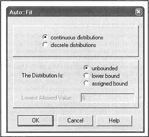
FIGURE 9.6 Auto Fit Dialogue Window

The results of the Auto Fit are shown in Figure 9.7. Stat::Fit tried to fit four different continuous distributions, and the Exponential distribution with a mean value of 98.5 was ranked the highest. The Lognormal distribution also is considered a good fit, but the Uniform and the Normal distributions are not.
The fitted distribution can be plotted to provide visual confirmation that these are good models for the input data. The plot of the input data and the fitted distribution is shown in Figure 9.8. This plot is constructed by the Graph Fit tool in the toolbar of Stat::Fit.
Instead of using the Auto::Fit function, it is possible to test the goodness of fit of a particular distribution, just as was done by hand in the previous subsection. To do this, open the Fit > Setup … dialogue, then select the distribution(s) to be tested in the Distributions tab and the tests to be performed in the Calculations tab. After choosing the Exponential distribution in the Distributions tab and the chi-square and KS tests in the Calculations tab, the results shown in Figure 9.9 were obtained. Note that the chi-square value calculated by Stat::Fit matches the one obtained in Table 9.4.
The results of the distribution fitting performed with Stat::Fit can be exported to Extend. To do this, open the dialogue File > Export > Export Fit or click on the Export button in the toolbar. Pick Extend under the application window and then choose the desired distribution. Next, click OK and go back to Extend. The Input Random Number block from which Stat::Fit was invoked will show the fitted distribution in the Distributions tab.
9.2.3 CHOOSING A DISTRIBUTION IN THE ABSENCE OF SAMPLE DATA
When using simulation for process design, it is possible (and even likely) to be in a situation where field data are not available. When this situation arises, it is necessary to take advantage of the expert knowledge of the people involved in the process under consideration. For example, the analyst could ask a clerk to estimate the length of a given activity in the process. The clerk could say, for instance, that the activity requires “anywhere between 5 and 10 minutes.” The analyst can translate this estimate into the use of a Uniform (or Rectangular) distribution with parameters 5 and 10 for the simulation model.

Sometimes process workers are able to be more precise about the duration of a given activity. For instance, a caseworker might say: “This activity requires between 10 and 30 minutes, but most of the time it can be completed in 25 minutes.” This statement can be used to model the activity time as a Triangular distribution with parameters (10, 25, 30), where a = 10 is the minimum, b = 30 is the maximum, and c = 25 is the mode. The additional piece of information (the most likely value of 25 minutes) allows the use of a probability distribution that reduces the variability in the simulation model when compared to the Uniform distribution with parameters 10 and 30.
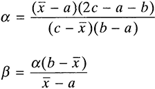
If the analyst is able to obtain three estimates representing the minimum, the maximum, and the most likely value, a generalization of the Triangular distribution also can be used. This generalization is known as the Beta distribution. The Beta distribution is determined by two shape parameters, α and β. Given these parameters the corresponding mean, µ, and mode, c, are obtained with the following mathematical expressions.

If an estimate x̅ of the true mean µ is available, along with an estimate of the mode c, the following relationships can be used to obtain the values of the α and β parameters for the Beta distribution.

The Beta distribution has some interesting properties. For example, the Beta distribution with parameters (1,1) is the same as the Uniform distribution with parameters (0,1). A beta random variable x in the interval from 0 to 1 can be rescaled and relocated to obtain a beta random variable in the interval between A and B with the transformation:
Also, the Beta distribution with parameters (1,2) is a left triangle, and the Beta distribution with parameters (2,1) is a right triangle. The selection of the parameter values for the Beta distribution can change the shape of the distribution drastically. For example,when x̅ is greater than c, the parameter values α and β calculated as shown previously result in a Beta distribution that is skewed to the right. Otherwise, the resulting Beta distribution is skewed to the left. A beta random variable can be modeled in Extend with an Input Random Number block from the Inputs/Outputs submenu of the Generic library. Figure 9.10 shows the dialogue screen for the Input Random Number block when the Beta distribution is chosen from the Distribution menu. The Shape1 parameter is α, the Shape2 parameter is β, and the Maximum and Location parameters are B and A as specified previously.
Example 9.4
Suppose an analyst would like to use the Beta distribution to simulate the processing time of an activity. No field data are available for a goodness-of-fit test, but the analyst was told that the most likely processing time is 18.6 minutes, with a minimum of 10 minutes and a maximum of 20 minutes. It is also known that the average time is 17.8 minutes. With this information, the analyst can estimate the value of the shape parameters as follows.

FIGURE 9.10 Beta Distribution Modeled with the Input Random Number Block


The shape of the Beta distribution with α = 1 and β = 2 is shown in Figure 9.11.
Note that the x values in Figure 9.11 range from 0 to 1. To obtain processing times in the range from 10 to 20 minutes, simply use the transformation 10 + (20 − 10)x.
9.3 Random Number Generators
Random numbers are needed to create computer simulations of business processes. The generation of random numbers is an important element in the development of simulation software such as Extend. The random number generators typically are hidden from the user of the simulation software, so it might seem that these numbers are generated magically and that there should be no concern regarding how they were obtained. However, random number generation is one of the most fundamental elements in computer based simulation techniques. For the conceptual understanding of this type of simulation methods, it is therefore imperative to address a few basic issues related to random number generators.
Computer software uses a numerical technique called pseudo-random number generation to generate random numbers. The word pseudo-random indicates that the stream of numbers generated using numerical techniques results in a dependency of the random numbers. In other words, numerical techniques generate numbers that are not completely independent from one another. Because the numbers are interlinked by the formulas used with a numerical technique, the quality of the stream of random numbers depends on how well the interdependency is hidden from the tests that are used to show that the stream of numbers is indeed random. Consider, for example, a simple but poor numerical technique for generating random numbers. The technique is known as the mid-square procedure.
- Select an n-digit integer, called the seed.
- Find the square of the number. If the number of digits of the resulting value is less than 2n, append leading zeros to the left of the number to make it 2n digits long.
- Take the middle n digits of the number found in step 2.
- Place a decimal point before the first digit of the number found in step 3. The resulting fractional number is the random number generated with this method.
- Use the number found in step 3 to repeat the process from step 2.
Example 9.5
Create a stream of five four-digit random numbers in the range from 0 to 1 using the midsquare procedure, starting with the seed value 4, 151.
Table 9.7 shows the stream of random numbers generated from the given seed. Note that the mid-square procedure can fail to generate random numbers if the seed is such that the square of the current number creates a pattern of a few numbers that repeat indefinitely. For example, if the seed 1,100 is used, the method generates the sequence 0.2100, 0.4100, 0.8100, 0.6100 and repeats this sequence indefinitely. The seed value of 5,500 always generates the same “random” number—0.2500. Try it!
TABLE 9.7 Random Number Generation with Mid-Square Procedure

Random number generators in simulation software are based on a more sophisticated set of relationships that provide a long stream of random numbers before the sequence of values repeats. One popular procedure is the so-called linear congruential method. The mathematical relationship used to generate pseudo-random numbers is:
The Z values are integer values with Z0 being the seed. The r-values are the random numbers in the range from 0 to 1. The mod operator indicates that Zi is the remainder of the division of the quantity between parentheses by the value of m. The parameter values a, c, and m as well as the seed are nonnegative integers satisfying 0 < m, a < m, c < m, and Z0 < m.
Example 9.6
Create a stream of five four-digit random numbers in the range from 0 to 1 using the linear congruential method with parameters a = 23, c = 7, m = 34, and a seed of 20.
| Z1 = (20 × 23 + 7) mod 34 = 25 | r1 = 25/34 = 0.7353 |
| Z2 = (25 × 23 + 7) mod 34 = 4 | r2 = 4/34 = 0.1176 |
| Z3 = (4 × 23 + 7) mod 34 = 31 | r3 = 31/34 = 0.9118 |
| Z4 = (31 57 × 23 + 7) mod 34 = 6 | r4 = 6/34 = 0.1765 |
| Z5 = (6 × 23 + 7) mod 34 = 9 | r5 = 9/34 = 0.2647 |
The linear congruential method may degenerate if the parameter values are not chosen carefully. For example, if the parameter m is changed to 24 in Example 9.6, the sequence of random numbers degenerates in such a way that 0.8333 and 0.4583 repeat indefinitely.
Numerical methods for generating pseudo-random numbers are subjected to a series of tests that measure their quality. High-quality generators are expected to create random numbers that are uniform and independent. The goodness-of-fit test can be used to check uniformity. The runs test typically is used to check dependency.
9.3.1 THE RUNS TEST
The runs test is used to detect dependency among values in a data set represented as a sequence of numbers. A run is a succession of an increasing or decreasing pattern in the sequence. The length of the run is given by the number of data points within one pattern before the pattern changes. Typically, the plus (+) sign is used to indicate a pattern of increasing numbers, and a minus (−) sign indicates a pattern of decreasing numbers. For example, the sequence 1, 7, 8, 6, 5, 3, 4, 10, 12, 15 has three runs:
First is an increasing pattern that changes when the sequence goes from 8 to 6. The decreasing pattern continues until the sequence goes from 3 to 4, from which the increasing pattern continues until the end of the sequence. Note that any sequence of n numbers cannot have more than n − 1 runs and less than 1 run.
The runs test is based on comparing the expected number of runs in a true random sequence and the number of runs observed in the data set. If R is the number of runs in a true random sequence of n numbers, then the expected value and the standard deviation of R have been shown to be:
Also, it has been shown that the distribution of R is Normal for n > 20. The runs test has the following form.
H0 : The sequence of numbers is independent
HA : The sequence of numbers is not independent
The following statistic is used to test this hypothesis:

where R is the number of runs in the data set with µR and σR computed as shown previously. The null hypothesis is not rejected at the a level of significance if the following relationship holds.
In other words, if the Z statistic falls outside the range specified by the level of significance, the hypothesis that the numbers in the sequence are independent is rejected.
Example 9.7
Consider the following sequence of 22 numbers. Perform the runs test to determine, with a 95 percent confidence level, whether or not the numbers in the sequence (ordered by rows) are independent.

The following represents the runs in the sequence.
Then, the number of runs R, the expected number of runs µR, and the standard deviation of the number of runs σR are:

The Z statistic is calculated as follows.
The critical value can be found from the Normal distribution tables (see the Appendix) or with the following Microsoft Excel function.
Because Z is within the interval defined by −Zα/2 and Zα/2, the null hypothesis, which states that the numbers in the sequence are independent, is not rejected.
9.4 Generation of Random Variates
The previous section showed two methods for generating random numbers uniformly distributed between 0 and 1. However, in most simulation models it is necessary to generate random numbers from probability distributions other than the Uniform (or Rectangular) distribution. Chapter 6, section 6.3.3 showed how a function transformation can be used to generate variates from the Exponential distribution. This technique is known as the inverse transformation technique. The technique takes advantage of the fact that cumulative distribution functions (CDFs) are defined in the range between 0 and 1. In addition, the CDF values corresponding to the values of the random variable are uniformly distributed, regardless of the probability distribution of the random variable. Mathematically, this is expressed as follows:
where F(x) is the cumulative distribution function of the random variable x, and r is a random number uniformly distributed between 0 and 1. If the CDF is known, then random variates of the random variable x can be found with the following inverse transformation.
Example 9.8
Use the uniform random numbers generated in Example 9.6 to generate variates of an exponentially distributed random variable with a mean of 10 minutes. The Exponential cumulative distribution function has the following form.
Applying the inverse transformation, the following is obtained.

Note that if r is a random variable uniformly distributed between 0 and 1, then 1 − r is also a random variable uniformly distributed between 0 and 1. Therefore, random variates of the Exponential distribution with mean value of 10 can be generated as follows.
| r1 = 0.7353 | x1 = −10 × 1(0.7353) = 3.075 |
| r2 = 0.1176 | x2 = −10 × (0.1176) = 21.405 |
| r3 = 0.9118 | x3 = −10 × (0.9118) = 0.923 |
| r4 = 0.1765 | x4 = −10 × (0.1765) = 17.344 |
| r5 = 0.2647 | x5 = −10 × 1/2(0.2647) = 13.292 |
Although the inverse transformation technique is a good method for generating random variates, there are some distributions for which the inverse of the CDF does not have a closed analytical form. For example, random variates of the Normal distribution cannot be obtained with a direct application of the inverse transformation technique. The technique can be applied using an approximation that takes advantage of the central limit theorem.
Fortunately, simulation software provides an automated way of generating random variates of the most popular theoretical distributions. In Extend, the Input Random Number block from the Inputs/Outputs submenu of the Generic library is used for the purpose of generating random variates from a catalog of well-known probability distribution functions. As shown in Figure 9.10, one simply selects the probability distribution from the drop-down menu and then enters the appropriate parameter values.
Occasionally, it is necessary to simulate processes for which some of the uncertainty is due to random variables with discrete probability distributions of an arbitrary form. For example, the transportation time from a distribution center to a customer could be specified as being 2 days 20 percent of time, 3 days 50 percent of the time, and 4 days 30 percent of the time. This distribution of times is clearly an arbitrary discrete probability distribution function. Table 9.8 shows the cumulative distribution function associated with the transportation times.
The inverse transformation technique can be used to generate random variates of an arbitrary discrete distribution function. Once again, a uniformly distributed random variable r is used. The transformation associated with the probability distribution in Table 9.8 is given in Table 9.9.
Example 9.9
Use the uniform random numbers generated in Example 9.6 to generate variates of the arbitrary discrete probability distribution function in Table 9.8. When the inverse transformation in Table 9.9 is applied to the uniform random numbers generated in Example 9.6, the following random variates are generated.
TABLE 9.8 Arbitrary Discrete PDF and CDF


| r1 = 0.7353 | x1 = 4 |
| r2 = 0.1176 | x2 = 2 |
| r3 = 0.9118 | x3 = 4 |
| r4 = 0.1765 | x4 = 2 |
| r5 = 0.2647 | x5 = 3 |
Extend provides an easy way of generating random variates from arbitrary discrete probability distribution functions. The Input Random Number block from the Inputs/Outputs submenu of the Generic library provides this functionality. Figure 9.12 shows the dialogue of the Input Random Number block when the Empirical Table is chosen from the Distribution menu and the Empirical Values option is set to Discrete.
The Input Random Number block also provides the functionality to generate random variates from an arbitrary continuous distribution. Suppose that instead of the discrete probability distribution in Table 9.8, one would like to use a continuous probability distribution of the following form.

FIGURE 9.12 An Arbitrary Discrete PDF Modeled with Extend
| f(x) = 0.2 | 1 ≤ x <2 |
| f(x) = 0.5 | 2 ≤ x <3 |
| f(x) = 0.3 | 3 ≤ x <4 |
The inverse transformation technique could be applied using integral calculus to find the inverse of the cumulative distribution function. In Extend, however, this arbitrary continuous distribution can be modeled easily with the Input Random Number block. The Empirical Table is chosen from the Distribution menu and then the Stepped option is used for the Empirical values. Figure 9.13 shows the dialogue for this Extend block along with the corresponding plot of the arbitrary continuous distribution.
Note that the first value in the Empirical Table of Figure 9.13 corresponds to the lower bound of the first range in the arbitrary continuous distribution (which is 1 in this case). The bounds of the subsequent ranges are given in order until the upper bound of the last range is reached (which is 4 in this case). Also note that the last two probability values are the same, indicating the end of the PDF.
9.5 Analysis of Simulation Output Data
The previous sections have addressed the issues associated with the modeling of process uncertainty using discrete-event simulation. The stochastic behavior of the output of a process is due to inputs (e.g., the uncertainty in the arrival of jobs) and internal elements (e.g., the uncertainty of processing times, the routing of jobs in the process, or the availability of resources). Hence, the output of a simulation model also should be treated as a set of random variables. For example, the waiting time of jobs is a random variable that depends on the inputs to the simulation model as well as the model’s internal elements. Other random variables that are outputs of process simulations are cycle time and work-in-process.
The goal of this section is to discuss some basic concepts of statistical analysis of data obtained from running a process simulation. In the context of business process design, simulation studies are performed for the following reasons.
- To estimate the characteristics (e.g., mean and standard deviation) of output variables (e.g., cycle time) given some input conditions and values of key parameter settings. This estimation helps one understand the behavior of an existing business process or predict the behavior of a proposed process design.
- To compare the characteristics (e.g., minimum and maximum) of output variables (e.g., resource utilization) given some input conditions and values of key parameter settings. These comparisons help one choose the best design out of a set of alternative process configurations. Also, the comparisons can be used to determine the best operating conditions for a proposed process design.
Statistical analysis of simulation output is necessary in order to draw valid conclusions about the behavior of a process. When performing statistical analysis, one must deal with the issu.es related to sampling and sample sizes. These issues cannot be ignored, because valid conclusions cannot be drawn from a single simulation run of arbitrary length. To illustrate the danger of ignoring proper statistical sampling techniques, consider the following example.
Example 9.10
A simulation model has been built to estimate the number of insurance policies that are in process at the end of a working day in an underwriting department. After running the simulation model one time, the WIP is estimated at 20 policies at the end of the day. However, making decisions based on this estimate would be a terrible mistake. First of all, this estimate is based on a single run that represents a day of operation starting with an empty process. In other words, the WIP is zero at the beginning of the simulation. If 30 days of operation are simulated by running the model 30 times, the wrong assumption would be made that the WIP is always zero at the beginning of each day. It would be assumed that the policies that were in process at the end of one day would disappear by the beginning of the next business day. What needs to be done is to run the simulation model for 30 × 8 = 240 hours and record the WIP at the end of each 8-hour period. After running this simulation, one would observe that the WIP at the end of the first day is 20, but the WIP at the end of the 30th day is 154 insurance policies. This might indicate that the process is not stable and that the WIP will keep increasing with the number of simulated days. This is confirmed by a simulation run of 300 days that results in a final WIP of 1,487 insurance policies.

The previous example illustrates the importance of choosing an appropriate value for the simulation length. Clearly in this example, simulating 10 days of operation was not enough to determine whether or not the current process configuration is indeed stable. The example also addresses the difference between a terminating and a nonterminating process. Figure 9.14 shows the types of statistical analysis associated with simulation models for terminating and nonterminating processes.
The following two subsections comment on the differences between the analyses that are appropriate for each of these simulation types.
9.5.1 NONTERMINATING PROCESSES
A nonterminating process is one whose operation does not end naturally within a practical time horizon. Many business processes are nonterminating. For example, order fulfillment, credit approval, and policy underwriting are nonterminating processes. These processes are correctly viewed as nonterminating, because the ending condition of the previous day is the beginning condition of the current day. Other systems such as traffic and telecommunications networks are clearly nonterminating because their operation is not divided into discrete units of time (such as working days). Most nonterminating processes eventually reach a steady state—a condition in which the process state distribution does no longer change with time and is no longer affected by the initial state in which the simulation was started. Example 9.10 is an illustration of a nonterminating process that doesn’t reach a steady state. Typically, nonterminating processes go through a transient period before reaching a steady state. An output variable, such as the utilization of a resource, exhibits a transient period at the beginning of a simulation before reaching a steady state that represents the long-term condition for the given resource.

FIGURE 9.14 Analysis of Output Data According to Simulation Characteristics
Determining the end of a transient period is an essential part of studying the steady-state behavior of a process. The data collected during a transient period belong to a different statistical population than data collected during a steady state. Mixing data from a transient period with data from the steady state results in unreliable estimates of key output statistics. Therefore, the steady-state analysis should be performed with data collected after the end of the transient period.
Some statistical techniques have been used to determine the end of the transient period. For example, the runs test has been applied for this purpose. A simple way of finding the transition between the transient period and a steady state is to examine a line plot of the output variable of interest. Figure 9.15 shows the cycle time values from a simulation of a given process. The figure also shows the cumulative average cycle time. Note that the running average has a smoother pattern of change, which makes it easier to identify underlying changes in the process behavior.
In the line graph depicted in Figure 9.15, a change in the cycle times can be identified at simulation time 15. After detecting the length of the transient period using a pilot run, additional runs can be made with instructions to the software to start data collection after the so-called warm-up period has ended. In Extend, this is done by connecting a Program block from the Generators submenu of the Discrete Event library and a Clear Statistics block from the Statistics submenu of the Generic library, as shown in Figure 9.16.
The blocks shown in Figure 9.16 clear the statistics computed during the warm-up period. If the warm-up period, for instance, is 15 minutes, then the Program block is set to generate an item with a value of 1 at time 15, as shown in Figure 9.17.

FIGURE 9.15 Line Plot of Cycle Times and Average Cycle Time


FIGURE 9.17 Program Block Scheduled to Generate an Item at Time 15
The item generated by the Program block is passed to the Clear Statistics block. The Clear Statistics block is set to clear the statistics in all the blocks that calculate them, as shown in Figure 9.18.
The initial conditions of the process generally affect the steady-state analysis. However, the effect of the initial conditions decreases with the length of the simulation. For simulation of an existing process, it is possible to use average values to create an initial condition for the simulation. For example, average values can be used to initialize the queues in a process in such a way that when the simulation starts, the process is not empty.
9.5.2 TERMINATING PROCESSES
A terminating process is one that typically starts from an empty state and ends also at an empty state. The termination of the process happens after a certain amount of time has elapsed. For example, the pet adoption process of a Humane Society (described in Chapter 8) starts at an empty state in the morning and closes after 8 hours of operation.

The state of a terminating process is empty when it closes. Terminating processes might or might not reach a steady state. Many terminating processes might not even have a steady state. To find out whether or not a terminating process has a steady state, a simulation model of the process can be executed beyond the natural termination of the process. For example, the pet adoption process mentioned previously could be simulated for 100 continuous hours to determine whether or not the process reaches a steady state. The steady-state behavior of a terminating process could be used to estimate critical measures of performance and make decisions about the configuration of such a process.
The estimation of performance for terminating processes is generally achieved with statistical analysis of multiple independent runs. In this case, the length of each run is determined by the natural termination of the process. The number of runs is set to collect enough data to perform statistical analysis that allows the analyst to draw valid conclusions about the performance of the process.
The amount of data available after a single run of a terminating process depends on the output variable under study. For example, suppose a simulation model of the aforementioned pet adoption process is run once and that 40 adoptions are completed. At the end of the run, a data set consisting of 40 observations is available for output variables such as cycle time and cycle time efficiency (because these values can be recorded for each completed adoption). On the other hand, there will be only a single observation of output variables such as daily throughput rate and overtime. In this case, a meaningful sample is taken, executing the simulation for a number of independent runs. Each run starts with the same initial conditions, but the runs use a different stream of random numbers. The Discrete Event tab of the Simulation Setup in the Run menu of Extend allows the number of runs for a single execution of the simulation model to be set. When more than one run is specified, the execution does not stop until all runs are completed. One run follows the next one, and the stream of random numbers is not reinitialized. Instead, each run uses a different section of the stream of random numbers that is seeded as specified in the Random Numbers tab of the Simulation Setup.
This method results in samples of random variables for which only one observation can be obtained per run. The samples consist of independent observations of the random variable. In addition, it is valid to assume that the observations are identically distributed. These properties make the application of traditional statistical methods for estimation and hypothesis testing a robust approach to analyze output simulation data.
Example 9.11
A project consists of seven activities with duration and precedence relationships given in Table 9.10.
The duration of each activity is a random variable as specified in Table 9.10. An activity can be started only after all preceding activities are completed. One of the main goals of project management is to estimate the duration of the project. When the duration of the activities in the project is uncertain, project managers often rely on a methodology called PERT (Project Evaluation and Review Technique) to obtain an estimate of the expected completion time and its associated standard deviation. PERT calculations assume that the activity times are distributed according to a Beta distribution. A minimum, a maximum, and a most likely value for the duration of each activity are used to perform the analysis. The advantage of using simulation in this context is that one does not have to assume that the activity times are beta distributed. An Extend model of this project is shown in Figure 9.19.
TABLE 9.10 Project Activities with Random Duration


FIGURE 9.19 Extend Model of a Project with Seven Activities

Note that the simulation model in Figure 9.19 uses a Timer block to calculate the completion time of the project. Then this value is passed to the File Output block from the Inputs/Outputs submenu of the Generic library. This block creates a file of all the data that are passed to it. The activities are modeled as hierarchical blocks containing an Input Random Number block from the Generic library and an Operation block from the BPR library. The simulation is executed 100 times, and the completion times are recorded in a file. Note that in this simulation, the sample can be collected by executing the model once with 100 arrivals generated with the Import block. A histogram over the sample data is shown in Figure 9.20.
The histogram in Figure 9.20 (constructed by importing the output file to Excel) shows that about 80 percent of the time, the project is completed within 35 days. The expected completion time is 29.8 days with a standard deviation of 7.6 days. In addition to calculating simple statistics, these sample data can be used to estimate confidence intervals, to calculate an appropriate sample size for a specified interval precision, and to test hypotheses, as presented in the following sections.
9.5.3 CONFIDENCE INTERVALS
Statistical estimation of characteristics (e.g., the mean) of a population is typically done in two ways: point estimates and confidence intervals. Point estimates are obtained by calculating statistics from a sample of the population. For example, the sample mean is an estimate of the true but unknown population mean. The average waiting time in a queue calculated from simulation output is a point estimate of the true but unknown mean of the population of all waiting times for the queue. Confidence intervals expand this analysis by expressing the estimates as intervals instead of single values. The intervals might or might not contain the true value of the parameter; however, a so-called confidence level represents the accuracy of the estimation. If two intervals have the same confidence level, the narrower of the two is preferred. Similarly, if two intervals have the same width, the one with a higher confidence level is preferred. Typically, the analyst chooses a desired confidence level and constructs an appropriate interval according to this selection.
The sample size and the standard deviation are the main factors that affect the width of a confidence interval. For a given confidence level, the following relationships hold.
- The larger the sample size is, the narrower the confidence interval is.
- The smaller the standard deviation is, the narrower the confidence interval is.
The first relationship generally is used to approach the estimation problem from the point of view of determining the sample size that will satisfy a set of requirements for the confidence interval. In other words, the analyst can specify a level of confidence and a desired width for the confidence interval first and then use this to determine a sample size.
Confidence Interval for a Population Mean
Mean values are often the focus of statistical analysis of simulation output. Average cycle time, average waiting time, average length of a queue, and average resource utilization are just a few examples of average values that are used to measure process performance. The most widely reported statistics associated with simulation output are the mean and the standard deviation. Suppose the values of an output variable are represented by x1, x2, …,xn (where n is the number of observations in the sample). The mean and the variance are estimated as follows.

If the random variables are independent and identically distributed, the distribution of the sample mean x̅ is Normal for a sufficiently large sample size (an often used rule of thumb is 30 observations or more). This is a result from the central limit theorem, which states that for a sufficiently large sample size, the distribution of the sample mean follows a Normal distribution regardless of the distribution of the individual observations, as long as they are independent and identically distributed. The random variable Z is defined as follows.

This random variable follows a standard normal distribution, meaning a Normal distribution with a mean of 0 and a standard deviation of 1. The population mean is represented by µ and σx̅ = σ/√n is the standard deviation of distribution of the sample mean. In this case, µ and σ are true but unknown parameters from the population. The mean value µ is the parameter that is to be estimated. If the population standard deviation σ is not known (as is typically the case), then it is possible to use the sample standard deviation s as a reasonable approximation as long as the sample size is large (at least 30). At a confidence level of 1 − α, a symmetrical confidence interval can be constructed from the following probability statement.
Then substitute the Z variable and solve for µ to obtain the confidence interval.

When the sample size is fewer than 30 observations, the use of the Normal distribution, as implied by the Central Limit Theorem, can be questionable. Instead of the Normal distribution, the Student t distribution can be employed in the following way.

This confidence interval based on the Student t distribution is exact only if the observed x-values are normally distributed. However, it is often used as an approximation when this condition is not satisfied. If we compare the critical values for the standard normal distribution with those obtained with the Student t distribution for a given confidence level, 1 − α, then tn−1,α/2 is strictly greater than Zα/2. Consequently, using the Student t distribution produces a wider confidence interval. This is why the Student t produces confidence intervals that are closer to the desired confidence level 1 − α when the sample size n is small. We also know that as the sample size becomes larger tn−1,α/2 approaches Zα/2. The critical values for the standard Normal distribution and the Student t distribution can be found in the Appendix. Alternatively, these values also can be found using the following Microsoft Excel functions.
Example 9.12
Table 9.11 shows 50 observations of the cycle time for a given business process. Construct a 95 percent confidence interval to estimate the true but unknown value of the mean cycle time for this process.
The point estimates for the mean and the standard deviation are x̅ = 7.418 and s = 1.565. The Z-value for a 95 percent confidence level is Z0975 = 1.96. Then, the 95 percent confidence interval for the population mean is:

TABLE 9.11 Sample Cycle Times

In Extend, the blocks Queue Stats, Activity Stats, Resource Stats, and Cost Stats from the Statistics submenu of the Discrete Event library automatically construct confidence intervals. Figure 9.21 shows the dialogue of a Queue Stats block after 20 runs of a simulated process.
The block in Figure 9.21 has recorded statistics of single Stack block labeled In Box. Because these data come from 20 independent runs, they can be used to set confidence intervals. The result of clicking on the Confidence Interval button of the Queue Stats block is shown in Figure 9.22. Using the data in Figure 9.21, one can verify that Extend constructed the confidence intervals using the equation with the t distribution as presented previously.
Confidence Interval for a Population Proportion
Some output variables from a process simulation are proportions. For example, in pet adoption processes, directors of operations of Humane Societies are interested in estimating the proportion of patrons who adopt a pet to the total of patrons who initiate the process. The percentage of jobs going through a specialized operation and the percentage of jobs requiring rework are two more examples of output variables that represent proportions. In general, a proportion is a value representing the percentage of one type of outcome (often referred to as success) in a number of trials.
The true but unknown probability of success is denoted by p. Therefore, the probability of failure is 1 − p. The resulting random variable takes on two values: zero with probability 1 − p and 1 with probability p. A random variable of this kind follows a Bernoulli distribution, for which the mean value is p and the variance is p(1 − p). In a sample of n observations, the ratio of the number of successes to the total number of trials p̅ is a point estimate of p. The distribution of the p̅ statistic is approximately Normal for n larger than 10 and both np > 5 and n(1 − p) > 5. A (1 − α) percent confidence interval for p can be constructed from the following probability statement.

FIGURE 9.21 Queue Stats Block After 10 Runs


Note that the probability statement requires the knowledge of p to be able to calculate the standard deviation. Because p is the parameter to be estimated, p̅ can be used to approximate p for the calculation of the standard deviation when the sample size is sufficiently large. Substituting p with p̅ in the denominator and rearranging the elements of the probability statement gives the following confidence interval for a proportion.
Example 9.13
Consider the cycle time data in Table 9.11. Suppose the proportion p of interest is the percentage of jobs whose cycle time is greater than 7. Suppose also that the goal is to construct a 99 percent confidence interval for p. Table 9.11 shows 28 observations with cycle time greater than 7; therefore, p̅ = 0.56. The resulting confidence interval is as follows.

Note that as in the case of the confidence interval for a population mean, the interval width is reduced as the number of observations in the sample is increased. The value of 2.576 in the aforementioned calculation is the Z value (obtained from Excel) that yields a cumulative probability of 0.995 in a standard Normal distribution.
9.5.4 SAMPLE SIZE CALCULATION
The previous section assumed that the sample size was a given value. In practice, however, one of the key issues in statistical analysis of simulation output is the determination of an appropriate sample size. The sample size is either related to the length of the simulation or the number of simulation runs, depending on the model. The theory of statistics includes what is known as the law of large numbers, which refers to the property that statistics calculated using large samples from independent random variables are nearly exact estimates of the population parameters. Today’s simulation software coupled with the power of state-of-the-art computer hardware makes it possible to perform many lengthy simulation runs within a reasonable amount of time. Nevertheless, the question of what can be considered a reasonably large sample size still remains. The answer depends on the variation of the random variable of interest.
An important issue in determining an appropriate sample size is the desired precision level. The analyst must set a desired width of the confidence interval and also specify a level of confidence. With this in place the equations derived in the previous section can be solved to determine the corresponding sample size. It is interesting to point out that the sample size cannot be determined before the simulation model is run a few times because an estimate of the standard deviation is needed to determine the sample size. So in practice, a provisional sample size is used for an initial run that can yield enough data to estimate the standard deviation. The resulting estimate is used to derive an appropriate sample size that in turn yields the necessary data for constructing the desired confidence interval.
Suppose the goal is to construct a confidence interval with a total width of 2d, where d is half of the interval’s width. The confidence interval for a population mean can be expressed as follows.
Comparing this inequality with the one derived in the previous section, one can write:

Because the true standard deviation is generally not known, the sample standard deviation s can be used to estimate it. The following equation is used to solve for the sample size.

The resulting sample size value guarantees a (1 − α) percent confidence interval of width 2d as long as the sample standard deviation represents a good estimate of the population standard deviation.
Consider once again the cycle time data in Table 9.11. The confidence interval constructed in Example 9.12 with these data has a total width of 0.868 (i.e., 2d = 0.868 or d = 0.434). Suppose one wants to construct a confidence interval with the same confidence level of 95 percent but with a total width of 0.6 (i.e., 2d = 0.6 or d = 0.3). Calculate the sample size needed to achieve the desired precision level.

A similar calculation can be made to find the sample size necessary to construct a confidence interval of a given precision for a population proportion. Again assume that the analyst desires a (1 − α) percent confidence interval with a total width of 2d. The confidence interval can be expressed as follows.
where
Solving for the sample size n, one obtains the following.

Note that in this calculation, it is also necessary to execute a preliminary simulation run to be able to estimate the true proportion p with the sample proportion p̅ . Because an estimated value is being used to calculate the sample size, the accuracy of the calculation depends on the accuracy of the estimate obtained after the preliminary run. A more conservative approach is to use the maximum standard deviation value instead of the one calculated with the available p̅ . The maximum standard deviation of 0.25 occurs when p = 0.5. Therefore, a conservative and accurate sample size calculation for constructing a confidence interval on a proportion is:
The advantage of using this equation is that it does not depend on any population parameters; therefore, the sample size can be calculated without performing a preliminary simulation run.
Example 9.15
Consider Example 9.13. Calculate a sample size needed to construct a 99 percent confidence interval with a total width of 0.2. Use the formula that considers maximum standard deviation of the population.

9.5.5 Hypothesis Testing
The previous sections addressed several issues associated with statistical estimation. However, sometimes it is important to not only estimate the value of a parameter but to test whether a parameter is equal to a critical value. Similarly, it might be interesting to test whether there is a difference between two parameters, such as the means of two design alternatives of the same process. The statistical background used to set up and perform tests of hypotheses is the same one used to establish confidence intervals. In particular, it is assumed that the sample means are normally distributed.
A hypothesis states a certain relationship about an unknown population parameter that might or might not be true. This relationship is known as the null hypothesis (denoted by H0). Because the test is based on estimated values, it is possible to commit errors. When the null hypothesis is true and the test rejects it, it is said to have committed a type I error. A type II error occurs when the test fails to reject a false null hypothesis. The level of significance of the test is denoted by α and is interpreted as the maximum risk associated with committing a type I error. The confidence level of the test is 1 − α.
Suppose x̅ is the mean and s is the standard deviation estimated from a sample of n observations. Also suppose that we would like to test the following hypothesis.
Then, the null hypothesis is rejected (with a significance level of a) if the following relationship does not hold.

This is a so-called two-tail test on a population mean. The two related one-tail tests are shown in Table 9.12.
In addition to testing if a population mean is equal, greater than, or less than a given value, it is sometimes desirable to be able to compare the difference between two means. This is particularly useful in the context of process design, where it might be necessary to show that a new design is better than an existing design in terms of a key output variable. Suppose µ1 is the population mean of a new process design and that its value is estimated with x̅1. Suppose also that µ2 is the population mean of the existing process design and its value is estimated with x̅2. Then the following two-tail test can be formulated.
TABLE 9.12 One-Tail Hypothesis Test on One Mean


The null hypothesis is rejected (with a significance level of α) if the following relationship does not hold:

where n1 and n2 are the sample sizes for each population, respectively. Also, s1 and s2 are the sample standard deviations for the populations. One-tail tests similar to those in Table 9.12 can be formulated for the difference between two means, as shown in Table 9.13.
Example 9.16
Consider the cycle time data in Table 9.11. A new design has been proposed for the process, and a computer simulation prototype has been built. The cycle times in Table 9.14 were obtained from running the simulation model of the proposed process design.
Does the mean cycle time in the proposed process represent an improvement over the mean cycle time of the existing process? To find out, one can test the null hypothesis µ1 − µ2 ≥ 0, where µ1 is the true but unknown mean cycle time for the existing process and µ2 is the true but unknown mean cycle time for the proposed process. Comparing with the expressions in Table 9.13 this corresponds to a one-tail test with a = 0. Assume that a significance level of 5 percent will be used for this test.
Using the sample data, calculate ![]() The test score is then calculated as follows.
The test score is then calculated as follows.
TABLE 9.14 Cycle Times for a Proposed New Process Design


From the Normal distribution table in the Appendix, one can obtain Z0.05 = 1.645. Because Z > Z0.05, the null hypothesis can be rejected. This conclusion is reached at the confidence level of 95 percent.
The Data Analysis Toolpack of Microsoft Excel provides a tool for performing hypothesis testing directly on an electronic spreadsheet. Assume that the data in Table 9.11 are copied onto an Excel spreadsheet in the range A1:A50. Also assume that the data in Table 9.14 are copied onto the same Excel spreadsheet in the range B1:B50. Select the Data Analysis item in the Tools menu. Then select t-Test: Two-Sample Assuming Unequal Variances. Note that at this point one cannot choose the Z test, because this test assumes that the variances are known. The estimates of the variance could be entered in the corresponding text boxes; however, it is preferable to let Excel calculate the variances and use the t statistic. (Recall that the values of the t distribution with more than 30 degrees of freedom are similar to the values of the standard Normal distribution.) Figure 9.23 shows the completed dialogue for the selected t test. Table 9.15 shows the results of the t-test.
The t statistic of 1.822 is identical to the Z statistic that was used before. The t critical one-tail value of 1.665 is similar to Z0.05 = 1.645. The one-tail test shows the rejection of the null hypothesis. It also shows that the null hypothesis would not be rejected at a significance level of 3.6 percent (see the P(T ≤ t) one-tail value in Table 9.15). The two-tail test shows that the null hypothesis µ1 − µ2 = 0 cannot be rejected because the t statistic (1.822) falls within the range (−1.992, 1.992). The two-tail null hypothesis would be rejected at a level of significance of 7.2 percent (as specified by the two-tail p-value in Table 9.15).

FIGURE 9.23 Excel Dialogue for a t Test of the Difference Between Two Population Means

9.6 Summary
This chapter presented some basic statistical analysis tools for input and output simulation data. On the input side, it was shown how goodness-of-fit tests can be employed to determine suitable distributions for random variables such as interarrival times and processing times. The chapter also explored the mechanics involved in the generation of uniformly distributed random numbers and random variates from well-known distributions.
On the output side, the focus was placed on the problem of estimation and hypothesis testing. These tools are necessary to be able to draw valid conclusions with respect to the performance of business processes.
9.7 References
Khoshnevis, B. 1994. Discrete systems simulation. New York: McGraw-Hill.
Law, A. M., and W. D. Kelton. 2000. Simulation modeling and analysis, 3rd edition. Boston: McGraw-Hill.
9.8 Exercises
- Use the chi-square goodness-of-fit test and a significance level of 0.1 to test the set of interarrival times in Table 9.16 for possible fit to the Exponential distribution.
- Use the chi-square goodness-of-fit test and a significance level of 0.05 to test the set of service times in Table 9.17 for possible fit to the Normal distribution.
- An analyst is interested in determining whether the Weibull distribution with parameters α = 6 and β = 10 is a good fit to the data set in Table 9.18. Use Microsoft Excel to perform a chi-square goodness-of-fit test to help the analyst make a decision.
TABLE 9.16 Interarrival Times for Exercise 1

TABLE 9.18 Data Set for Exercise 3

- Use the Kolmogorov-Smirnov test to examine under the significance level of 0.01 whether the observations in Table 9.19 are random numbers uniformly distributed between 0 and 1.
- Apply the Kolmogorov-Smirnov test to the data in Exercise 1.
- Apply the Kolmogorov-Smirnov test to the data in Exercise 2.
- Consider the data in Exercise 4. Perform the runs test to determine with a 95 percent confidence level whether or not the numbers in the sequence (ordered by rows) are independent.
- The data set in Table 9.20 consists of cycle times of jobs in a given process. Perform the runs test to determine with a 99 percent confidence level whether or not the cycle times (ordered by columns) are independent.
- Starting with a seed of 3,461, generate 10 four-digit random numbers using the mid-square method.
- Use the linear congruential method with parameters Z0 = 79, a = 56214, c = 17, and m = 999 to generate 10 three-digit random numbers.
- Perform the following tests on the numbers generated in Exercise 10.
- Test for randomness using Kolmogorov-Smirnov with a significance level of 0.05.
- Test for independence using the runs test with a 0.05 level of significance.
TABLE 9.19 Data Set for Exercise 4

TABLE 9.20 Cycle Times for Exercise 8

TABLE 9.22 WIP Data for Exercise 14

- Use the data in Exercise 4 to generate random variates from the discrete probability distribution function in Table 9.21.
- Use the data in Exercise 4 to generate random variates from an Exponential distribution with a mean of 25.
- The data set in Table 9.22 represents the work-in-process (WIP) at the end of a day for a 40-day simulation of a given business process. Find a 99 percent confidence interval for the mean WIP.
- An analyst has suggested a new design for the process in Exercise 14. A simulation of the proposed process yielded the WIP values in Table 9.23. Test the hypothesis that the new process has a mean WIP that is less than the average of the old process. Assume a 5 percent significance level.
- With a preliminary simulation of 10 days of operation of an emergency room; an analyst found the results, shown in Table 9.24, in terms of the average number of patients waiting. Suppose the analyst would like to estimate the average number of patients waiting with a 95 percent confidence interval whose total width is four patients. Calculate the number of times the model must be run to be able to construct the desired confidence interval.
- (Adapted from Khoshnevis, 1994) The management of a major ski resort wants to simulate the rental program during the high season. The resort has two types of customers: people who pay cash and people who use a credit card. The interarrival times of these customers is exponentially distributed with means of 130 seconds and 60 seconds, respectively. After arrival, customers must fill out a waiver form. The time taken to fill out the waiver form is normally distributed with a mean of 60 and a standard deviation of 20 seconds.
TABLE 9.23 WIP Data for Exercise 15

After filling out the form, customers get in line to pay. Time to pay depends on the method of payment. The time required to pay in cash is uniformly distributed between 30 and 45 seconds; the time required to pay by credit card is uniformly distributed between 90 and 120 seconds.
Three types of rental equipment—boots, skis, and poles—are rented in that order in frequency. Not everyone rents all three types of equipment because some people already have some of the equipment. After paying, 80 percent of the people rent boots, 10 percent go directly to skis, and the rest only rent poles. At the boot counter, an employee takes a normally distributed time with a mean of 90 and a standard deviation of 5 seconds to obtain the boots for each customer. The time to try the boots is uniformly distributed between 60 and 240 seconds. About 20 percent of the people need a different size boot; the rest go to get their skis.
At the ski rental counter, everyone waits until a resort employee is free to obtain the right size ski, which takes a uniformly distributed time between 45 and 75 seconds. Twenty percent of these people need their bindings adjusted. The binding-adjustment process is exponentially distributed with a mean of 180 seconds. (The binding-adjustment process is considered separately in terms of staffing.) Seventy percent of the people go on to get poles; the rest leave. Ninety percent of the people who get their bindings adjusted go on to get poles, and the rest leave. At the station where the poles are rented, service is normally distributed with a mean of 60 and a standard deviation of 10 seconds.
- Assume that one employee is located in each service station (one at the cash register, one at the boots counter, one at the skis counter, and one at the poles). Simulate this process for 60 days and collect the daily average cycle time. Set a 95 percent confidence interval with the data collected during the simulation.
- Test the hypothesis (using a 5 percent significance level) that a difference in the mean cycle time results when one employee is added to the boots counter.
- Test the hypothesis (using a 5 percent significance level) that a difference in the mean cycle time results when one employee is added to the ski counter.
- Test the hypothesis (using a 5 percent significance level) that a difference in the mean cycle time results when two employees are added, one to the boots counter and one to the ski counter.
- The management of a mortgage company has decided, with limited information, that the company can save money if it reduces its staff size. Before downsizing, management asks you to model the credit application process to provide reassurance that service will not be severely affected by the reduction in staff.
The mortgage company currently employs three loan agents, two of whom perform an initial review of credit applications and a third who performs a second review of the applications that fail the initial review. The second review is performed in an attempt to correct the deficiencies by contacting the originating party. The process has the following characteristics.
- Approximately four to eight credit applications (and most likely six) arrive every hour.
- It takes 12 to 16 minutes to complete the first review.
- About 20 percent of the applications fail the first review.
- It takes 25 to 35 minutes to complete the second review.
- About 50 percent of the applications fail the second review.
Your task is to compare the performance of the current process with the performance of the process with two loan agents. For the downsized process, management wants the two remaining loan agents to work in either of the two reviewing steps. That is, the loan agents are not assigned to the first or second review step, but rather they perform initial or second reviews as needed.
- Create a simulation model of the current process. Use the Triangular distribution to model the arrivals of credit applications and the Rectangular distribution for the reviewing times.
- Simulate the process for 45 working days. (A working day is 8 hours of operation.) For each day, collect the average utilization of loan agents and the average cycle time.
- Modify the model to simulate the downsized process. Repeat part b for the new model.
- Use the runs test to determine whether the utilization average values are independent at a significance level of 0.05. Perform the same test for the cycle time averages. If the observations are independent, then perform a test of hypotheses to determine whether the overall mean utilization has changed from the current to the proposed process. Perform the same test for the overall average cycle time.


CASES
Simulation Project Improving the Process at County Hospital
County Hospital wishes to improve the service level of its regular X-ray operation, which runs from 8 A.M. to 8 P.M. Patients have identified the total required time as their main concern with this process. Management, on the other hand, is concerned with utilization of available resources. Management has created a process-improvement team to study this problem. The process might be redesigned as a result of the team’s recommendations.
The team has defined the entry point to the X-ray process to be the instant a patient leaves the physician’s office en route to the X-ray lab. The exit point has been defined as the instant at which the patient and the completed X-ray enter the physician’s office.
Broadly speaking, two types of patients arrive to the X-ray process: emergency and nonemergency patients (priority levels 1 and 2, respectively). The emergency patients arrive according to a Poisson process with a mean of four patients per hour. The nonemergency patients are registered as they enter, and a sample of the arrival time data is provided in Table 9.25. Until now, no attempt has been made to further analyze this data, so there is no insight into what the arrival process looks like.
The team has identified 12 activities in the current X-ray process (see Table 9.26), which is the same irrespective of the patient type. The only differences between patient categories are the activity times and their distributions, specified in Table 9.27.
The patient priority levels determine the service order of all the X-ray activities. Emergency patients (priority 1) come first at the expense of nonemergency patients (priority 2). However, after service is started, it will never be interrupted to benefit a high-priority patient.
The resource data for the X-ray process is specified in Table 9.28. The orderlies will always take one patient back from the X-ray lab when they have dropped one off. Assume that the transportation time back from the X-ray lab is exactly the same as the transportation time to the X-ray lab. If no patient is ready to go back, the orderly will wait for 5 minutes; if no patient becomes available during this time, the orderly will return to the ward without a patient. The time for an orderly to walk back without a patient is always 5 minutes. The orderlies will never go and pick up a patient at the X-ray area without bringing another patient with them from the ward.
PART I: ANALYZING THE CURRENT PROCESS DESIGN
- Draw a flowchart of the current X-ray process.
- Develop a simulation model of this process.
- The model requires analysis of input data regarding the arrival process of nonemergency patients.
- Modeling Hint: For batching and unbatching, use the blocks Batch and Unbatch from the Discrete Event library with the option Preserve Uniqueness checked.
- Modeling Hint: Build the model incrementally based on your flowchart. Do not try to put everything together at once and then test whether it works. The key is to use individual, small steps.
- As a first check that everything works as it is supposed to, it is often useful to run a shorter simulation with animation. Use different symbols for different types of items, such as different types of labor and different types of jobs.
- As a first-cut analysis, run a 1-day simulation with the random seed set at 100, using the correct activity time distributions. Look at the average cycle time, the throughput rate, the resource, the queue, and the activity statistics. What are the problems in this process?
- Simulate 30 days of operation and compute the cycle time and daily throughput (average and standard deviation). Also compute the activity and resource utilization statistics and queue statistics with 95 percent confidence intervals. (Use the Statistics blocks in the Discrete Event library of Extend.) Assume that any patients remaining in the system at the end of the day will be taken care of by the night shift. Every morning, the system is assumed to be empty. Are there any surprises when you compare these results with the ones in question 3?
- Assess the performance of the process using the values calculated in question 4. Where is the bottleneck? What is the problem area in terms of reducing the cycle time and increasing the throughput rate?
PART II: SUGGEST AND EVALUATE A NEW PROCESS DESIGN
- Based on your insight about the current operations, identify a plausible way of reducing the average cycle time by redesigning the process. For example: What happens if the X-ray technician no longer has to stay with the patient while the X-rays are developed? What if the messenger batch size changes? Is the messenger service necessary? What if more personnel are hired? What type of personnel would be most useful?
TABLE 9.27 Resource Data for X-Ray Process

- Investigate the performance of the redesigned process in terms of the cycle time and the daily throughput. Also look at the resource and activity utilization statistics and queue statistics with 95 percent confidence intervals as before. What are your conclusions? Is the new design significantly better than the old process with regards to the cycle time and throughput? Are any drawbacks obvious?


