6
Unbiased FIR State Estimation
The arithmetic mean is the most probable value.
Carl F. Gauss [53], p. 244
It is usually taken for granted that the right method for determining the constants is the method of least squares.
Karl Pearson [146], p. 266
6.1 Introduction
Optimal state estimation requires information about noise and initial values, which is not always available. The requirement of initial values is canceled in the optimal unbiased or ML estimators, which still require accurate noise information. Obviously, these estimators can produce large errors if the noise statistics are inaccurate or the noise is far from Gaussian. In another extreme method of state estimation that gives UFIR estimates corresponding to the LS, the observation mean is tracked only under the zero mean noise assumption. Designed to satisfy only the unbiasedness constraint, such an estimator discards all other requirements and in many cases justifies suboptimality by being more robust. The great thing about the UFIR estimator is that, unlike OFIR, OUFIR, and ML FIR, it only needs an optimal horizon of ![]() points to minimize MSE. It is worth noting that determining
points to minimize MSE. It is worth noting that determining ![]() requires much less effort than noise statistics. Given
requires much less effort than noise statistics. Given ![]() , the UFIR state estimator, which has no other tuning factors, appears to be the most robust in the family of linear state estimators.
, the UFIR state estimator, which has no other tuning factors, appears to be the most robust in the family of linear state estimators.
In this chapter, we discuss different kinds of UFIR state estimators, mainly filters and smoothers and, to a lesser extent, predictors.
6.2 The a posteriori UFIR Filter
Let us consider an LTV system represented in discrete‐time state space with the following state and observation equations, respectively,
These equations can be extended on ![]() as
as
using the definitions of vectors and matrices given for (4.7) and (4.14).
6.2.1 Batch Form
The unbiased filtering problem can be solved if our goal is to satisfy only the unbiasedness condition
and then minimize errors by choosing the optimal horizon of ![]() points.
points.
For the FIR estimate defined as
and the state model represented with the ![]() th row vector in (6.3),
th row vector in (6.3),
the condition (6.5) gives two unbiasedness constraints,
By multiplying both sides of (6.8) from the right‐hand side by the matrix identity ![]() and discarding the nonzero
and discarding the nonzero ![]() on both sides, we find the fundamental gain
on both sides, we find the fundamental gain ![]() of the UFIR filter
of the UFIR filter
where ![]() . Then, referring to the forced gain
. Then, referring to the forced gain ![]() given by (6.9), the a posteriori UFIR filtering estimate can be written as
given by (6.9), the a posteriori UFIR filtering estimate can be written as
As can be seen, the gain ![]() (6.10a) does not contain any information about noise and initial values, which means that the UFIR filter does not have the inherent disadvantages of the KF and OFIR filter.
(6.10a) does not contain any information about noise and initial values, which means that the UFIR filter does not have the inherent disadvantages of the KF and OFIR filter.
The error covariance for the a posteriori UFIR filter (6.11) can be written similarly to the OFIR filter (4.31) as
where the error residual matrices are given by
It now follows that (6.12) has the same structure as (4.55) of the a posteriori OUFIR filter with, however, another gain ![]() in (6.13) and (6.14).
in (6.13) and (6.14).
Because ![]() given by (6.10a) does not require noise covariances, the UFIR filter is not optimal and therefore generally gives larger errors than the OUFIR filter. In practice, however, this flaw can be ignored if a higher robustness is required, as in many applications, especially industrial.
given by (6.10a) does not require noise covariances, the UFIR filter is not optimal and therefore generally gives larger errors than the OUFIR filter. In practice, however, this flaw can be ignored if a higher robustness is required, as in many applications, especially industrial.
Generalized Noise Power Gain
An important indicator of the effectiveness of FIR filtering is the NPG introduced by Trench in [198]. The NPG is the ratio of the output noise variance ![]() to the input noise variance
to the input noise variance ![]() , which is akin to the noise figure in wireless communications. For white Gaussian noise, the NPG is equal to the sum of the squared coefficients of the FIR filter impulse response
, which is akin to the noise figure in wireless communications. For white Gaussian noise, the NPG is equal to the sum of the squared coefficients of the FIR filter impulse response ![]() ,
,
which is the squared norm of ![]() .
.
In state space, the homogeneous gain ![]() represents the coefficients of the FIR filter impulse response. Therefore, the product
represents the coefficients of the FIR filter impulse response. Therefore, the product ![]() plays the role of a generalized NPG (GNPG) [179]. Referring to (6.10a) and (6.10b), GNPG can be written in the following equivalent forms:
plays the role of a generalized NPG (GNPG) [179]. Referring to (6.10a) and (6.10b), GNPG can be written in the following equivalent forms:
It follows that GNPG is a symmetric square matrix ![]() , where the main diagonal components represent the NPGs for the system states, and the remaining components the cross NPGs. The main property of
, where the main diagonal components represent the NPGs for the system states, and the remaining components the cross NPGs. The main property of ![]() is that its trace decreases with increasing horizon length, which provides effective noise reduction. On the other hand, an increase in
is that its trace decreases with increasing horizon length, which provides effective noise reduction. On the other hand, an increase in ![]() causes an increase in bias errors, and therefore
causes an increase in bias errors, and therefore ![]() must be optimally set by choosing an optimal horizon length.
must be optimally set by choosing an optimal horizon length.
6.2.2 Iterative Algorithm Using Recursions
Recursions for the batch a posteriori UFIR filtering estimate (6.11) can be found by decomposing (6.11) as ![]() , where
, where
![]() is the homogeneous estimate and
is the homogeneous estimate and ![]() is the forced estimate.
is the forced estimate.
Using (6.16b), the estimate ![]() can be transformed to
can be transformed to

and, by applying the decomposition
the recursion for the GNPG (6.16b) can be obtained if we transform ![]() as
as

This gives the following forward and backward recursive forms:
Using (6.20) and (6.22) and extracting ![]() from (6.10a), we next transform the product
from (6.10a), we next transform the product ![]() as
as

By combining (6.21) and (6.23), we finally obtain the following recursion for the homogeneous estimate

where ![]() is the bias correction gain of the UFIR filter.
is the bias correction gain of the UFIR filter.
To find the recursion for the forced estimate (6.18), we first show that

Then, by extracting ![]() from (6.19),
from (6.19), ![]() can be transformed as
can be transformed as

Now, by combining (6.25) and (6.26) and substituting (6.22), the forced estimate (6.18) can be represented with the recursion
which, together with (6.24), gives the recursions for the a priori and a posteriori UFIR filtering estimates, respectively,
The recursive computation of the a posteriori UFIR filtering estimate (6.11) can now be summarized with the following theorem.
Note that the need to compute the initial ![]() and
and ![]() in short batch forms arises from the fact that the inverse in (6.16c) does not exist on shorter horizons.
in short batch forms arises from the fact that the inverse in (6.16c) does not exist on shorter horizons.
Modified GNPG
It was shown in [50,195] that the robustness of the UFIR filter can be improved by scaling the GNPG (6.21) with the weight ![]() as
as
The weight ![]() is defined by
is defined by

where ![]() ,
, ![]() is the integer part of
is the integer part of ![]() , and
, and ![]() is the number of the states. The RMS deviation
is the number of the states. The RMS deviation ![]() of the estimate is computed using the innovation residual as
of the estimate is computed using the innovation residual as
where ![]() means the dimension of the target motion. With this adaptation of the GNPG to the operation conditions, the UFIR filter can be approximately twice as accurate as the KF when tracking maneuvering targets [50].
means the dimension of the target motion. With this adaptation of the GNPG to the operation conditions, the UFIR filter can be approximately twice as accurate as the KF when tracking maneuvering targets [50].
6.2.3 Recursive Error Covariance
Although the UFIR filter does not require error covariance ![]() to obtain an estimate,
to obtain an estimate, ![]() may be required to evaluate the quality of the estimate on a given horizon. Since the batch form (6.12) is not always suitable for fast estimation, next we present the recursive forms obtained in [226].
may be required to evaluate the quality of the estimate on a given horizon. Since the batch form (6.12) is not always suitable for fast estimation, next we present the recursive forms obtained in [226].
Consider ![]() given by (6.12) and represent with
given by (6.12) and represent with
where the components are defined as

Using the decomposition ![]() , we represent matrix
, we represent matrix ![]() recursively as
recursively as
Then, referring to (6.20), (6.22), (6.31), and

and substituting ![]() with
with ![]() , we represent matrices
, we represent matrices ![]() and
and ![]() recursively with
recursively with


Similarly, the recursions for ![]() and
and ![]() can be obtained as
can be obtained as


By combining (6.31), (6.34), (6.35), and (6.36) with (6.30), we finally arrive at the recursive form for the error covariance ![]() of the a posteriori UFIR filter
of the a posteriori UFIR filter

It is worth noting that (6.37) is equivalent to the error covariance of the a posteriori KF (3.77), in which the Kalman gain ![]() must be replaced with the bias correction gain
must be replaced with the bias correction gain ![]() of the UFIR filter. The notable difference is that the Kalman gain minimizes the MSE and is thus optimal, whereas the
of the UFIR filter. The notable difference is that the Kalman gain minimizes the MSE and is thus optimal, whereas the ![]() derived from the unbiased constraint (6.17) makes the UFIR estimate truly unbiased, but noisier, since no effort has been made so far to minimize error covariance. The minimum MSE can be reached in the UFIR filter output at an optimal horizon of
derived from the unbiased constraint (6.17) makes the UFIR estimate truly unbiased, but noisier, since no effort has been made so far to minimize error covariance. The minimum MSE can be reached in the UFIR filter output at an optimal horizon of ![]() points, which will be discussed next.
points, which will be discussed next.
6.2.4 Optimal Averaging Horizon
Unlike KF, which has IIR, the UFIR filter operates with data on the horizon ![]() of
of ![]() points, which is sometimes called the FIR filter memory. To minimize MSE,
points, which is sometimes called the FIR filter memory. To minimize MSE, ![]() should be optimally chosen as
should be optimally chosen as ![]() . Otherwise, if
. Otherwise, if ![]() , noise reduction will be ineffective, and, for
, noise reduction will be ineffective, and, for ![]() , bias errors will prevail as shown in Fig. 6.1.
, bias errors will prevail as shown in Fig. 6.1.

Figure 6.1 The RMSE produced by the UFIR filter as a function of  . An optimal balance is achieved when
  , where the UFIR estimate is still less accurate than the KF estimate.
Since the UFIR filter is not selective, there is no exact relationship between filtering order and memory. Optimizing the memory of a UFIR filter in state space requires finding the derivative of the trace ![]() of the error covariance with respect to
of the error covariance with respect to ![]() , which is problematic, especially for LTV systems. In some cases,
, which is problematic, especially for LTV systems. In some cases, ![]() can be found heuristically for real data. If a reference model or the ground truth is available at the test stage, then
can be found heuristically for real data. If a reference model or the ground truth is available at the test stage, then ![]() can be found by minimizing
can be found by minimizing ![]() . For polynomial models,
. For polynomial models, ![]() was found in [169] analytically through higher order states, which has explicit limitations. If the ground truth is not available, as in many applications, then
was found in [169] analytically through higher order states, which has explicit limitations. If the ground truth is not available, as in many applications, then ![]() can be measured via the derivative of the trace of the measurement residual covariance, as shown in [153]. Next we will discuss several such cases based on the time‐invariant state‐space model
can be measured via the derivative of the trace of the measurement residual covariance, as shown in [153]. Next we will discuss several such cases based on the time‐invariant state‐space model
All methods will be separated into two classes depending on the operation conditions: with and without the ground truth.
Available Ground Truth
When state ![]() is available through the ground truth measurement, which means that
is available through the ground truth measurement, which means that ![]() is also available,
is also available, ![]() can be found by referring to Fig. 6.1 and solving on
can be found by referring to Fig. 6.1 and solving on ![]() the following optimization problem
the following optimization problem
There are several approaches to finding ![]() using (6.40).
using (6.40).
- When
 in (6.40) reaches a minimum with
  , we can assume that
  and represent the error covariance (6.37) by the discrete Lyapunov equation (A.34)
where
and represent the error covariance (6.37) by the discrete Lyapunov equation (A.34)
where  is required to be stable and matrix
  is symmetric and positive definite. Note that the bias correction gain
  in (6.41) is related to GNPG
  , which decreases as the reciprocal of
  . The solution to (6.41) is given by the infinite sum [83]
whose convergence depends on the model. The trace of (6.42) can be plotted, and then
. The solution to (6.41) is given by the infinite sum [83]
whose convergence depends on the model. The trace of (6.42) can be plotted, and then  can be determined at the point of minimum. For some models,
  can be found analytically using (6.42) [169].
 - For
 given by (6.37), the optimization problem (6.40) can also be solved numerically with respect to
  by increasing
  until
until  reaches a minimum. However, for some models, there may be ambiguities associated with multiple minima. Therefore, to make the batch estimator as fast as possible,
  should be determined by the first minimum [153]. It is worth noting that the solution (6.42) agrees with the fact that when the model is deterministic,
  and
and  , and the filter is a perfect match, then we have
  and
and  .
. - From Fig. 6.1 and many other investigations, it can be concluded that the difference between the KF and UFIR estimates vanishes on larger horizons,
 [179]. Furthermore, the UFIR filter is low sensitive to
  ; that is, this filter produces acceptable errors when
  changes up to 30% around
  [179]. Thus, we can roughly characterize errors in the UFIR estimate at
  in terms of the error covariance of the KF. If the product
  is invertible, then replacing the Kalman gain
  with the bias correction gain
  in the error covariance of the KF as
  and then providing simple transformations give
where
 is prior error covariance of the KF. For the given (6.43), the backward recursion (6.22) can be used to compute the GNPG back in time as(6.44)
Because an increase in
 always results in a decrease in the trace of
  [179], then it follows that
  can be estimated by calculating the number of steps backward until
  finally becomes singular. Since
  is singular when
  , where
  is the number of the states, the optimal horizon can be measured as
  . This approach can serve when
  or when there are enough data points to find
  . Its advantage is that
  can be found even for LTV systems.

The previously considered methods make it possible to obtain ![]() by minimizing
by minimizing ![]() . However, if the ground truth is unavailable and the noise covariances are not well known, then
. However, if the ground truth is unavailable and the noise covariances are not well known, then ![]() measured in this ways may be incorrect. If this is the case, then another approach based on the measurement residual rather than the error covariance may yield better results.
measured in this ways may be incorrect. If this is the case, then another approach based on the measurement residual rather than the error covariance may yield better results.
Unavailable Ground Truth
In cases when the ground truth is not available, ![]() can be estimated using the available measurement residual covariance
can be estimated using the available measurement residual covariance ![]() [153]. To justify the approach, we represent
[153]. To justify the approach, we represent ![]() as
as

where the two last terms strongly depend on ![]() . Now, three limiting cases can be considered:
. Now, three limiting cases can be considered:
- When
 , the UFIR filter degree is equal to the number of the data points, noise reduction is not provided, and the error
  with the sign reversed becomes almost equal to the measurement noise
  . Replacing
  with
with  makes (6.45) close to zero
- At the optimal point
 , the last two terms in (6.45) vanish by the orthogonality condition, the measurement noise prevails over the estimation error,
  , and the residual becomes
- When
 , the estimation error is mainly associated with increasing bias errors. Accordingly, the first term in (6.45) becomes dominant, and
  approaches it,
The transition between the ![]() values can be learned if we take into account (6.46), (6.47), and (6.48). Indeed, when
values can be learned if we take into account (6.46), (6.47), and (6.48). Indeed, when ![]() , the bias errors are practically insignificant. They grow with increasing
, the bias errors are practically insignificant. They grow with increasing ![]() and approach the standard deviation in the estimate at
and approach the standard deviation in the estimate at ![]() when the filter becomes slightly inconsistent with the system due to process noise.
when the filter becomes slightly inconsistent with the system due to process noise.
Since ![]() decreases monotonously with increasing
decreases monotonously with increasing ![]() due to noise reduction,
due to noise reduction, ![]() is also a monotonic function when
is also a monotonic function when ![]() . It grows monotonously from
. It grows monotonously from ![]() given by (6.46) to
given by (6.46) to ![]() given by (6.47) and passes through
given by (6.47) and passes through ![]() with a minimum rate when
with a minimum rate when ![]() is minimum. It matters that the rate of
is minimum. It matters that the rate of ![]() around
around ![]() cannot be zero due to increasing bias errors. And this is irrespective of the model, as the UFIR filter reduces white noise variance as the reciprocal of
cannot be zero due to increasing bias errors. And this is irrespective of the model, as the UFIR filter reduces white noise variance as the reciprocal of ![]() , and the effect of bias is still small when
, and the effect of bias is still small when ![]() .
.
Another behavior of ![]() can be observed for
can be observed for ![]() , when the bias errors grow not equally in different models. Although
, when the bias errors grow not equally in different models. Although ![]() is always convex on
is always convex on ![]() in stable filters, bias errors affecting its ascending right side can grow either monotonously in polynomial models or eventually oscillating in harmonic models. The latter means that
in stable filters, bias errors affecting its ascending right side can grow either monotonously in polynomial models or eventually oscillating in harmonic models. The latter means that ![]() can reach its value (6.48) with oscillations, even having a constant average rate.
can reach its value (6.48) with oscillations, even having a constant average rate.
It follows from the previous that the derivative of ![]() with respect to
with respect to ![]() can pass through multiple minima and that the first minimum gives the required value of
can pass through multiple minima and that the first minimum gives the required value of ![]() . The approach developed in [153] suggests that
. The approach developed in [153] suggests that ![]() can be determined in the absence of the ground truth by solving the following minimization problem
can be determined in the absence of the ground truth by solving the following minimization problem
where minimization should be ensured by increasing ![]() , starting from
, starting from ![]() , until the first minimum is reached. To avoid ambiguity when solving the problem (6.49), the number of points should be large enough. Moreover,
, until the first minimum is reached. To avoid ambiguity when solving the problem (6.49), the number of points should be large enough. Moreover, ![]() may require smoothing before applying the derivative.
may require smoothing before applying the derivative.
Let us now look at the ![]() properties in more detail and find a stronger justification for (6.49). Since the difference between the a priori and a posteriori UFIR estimates does not affect the dependence of
properties in more detail and find a stronger justification for (6.49). Since the difference between the a priori and a posteriori UFIR estimates does not affect the dependence of ![]() on
on ![]() , we can replace
, we can replace ![]() with
with ![]() ,
, ![]() with
with ![]() , and
, and ![]() with
with ![]() . We also observe that, since
. We also observe that, since ![]() ,
, ![]() ,
, ![]() , and
, and ![]() can be replaced by the UFIR estimate (6.29), the last two terms in (6.45) can be represented as
can be replaced by the UFIR estimate (6.29), the last two terms in (6.45) can be represented as

This transforms (6.45) to
Again we see the same picture. By ![]() , the bias correction gain in the UFIR filter is close to unity,
, the bias correction gain in the UFIR filter is close to unity, ![]() , and (6.50) gives a value close to zero, as in (6.46). When
, and (6.50) gives a value close to zero, as in (6.46). When ![]() ,
, ![]() and
and ![]() are small enough and (6.50) transforms into (6.47). Finally, for
are small enough and (6.50) transforms into (6.47). Finally, for ![]() ,
, ![]() becomes large and
becomes large and ![]() small, which leads to (6.48).
small, which leads to (6.48).
Although we have already discussed many details, it is still necessary to prove that the slope of ![]() is always positive up to and around
is always positive up to and around ![]() and that this function is convex on
and that this function is convex on ![]() . To show this, represent the derivative of
. To show this, represent the derivative of ![]() as
as ![]() , assuming a unit time‐step for simplicity. For (6.50) at the point
, assuming a unit time‐step for simplicity. For (6.50) at the point ![]() we have
we have ![]() and, therefore,
and, therefore, ![]() can be written as
can be written as
Since the GNPG ![]() decreases with increasing
decreases with increasing ![]() , then we have
, then we have ![]() , and it follows that
, and it follows that ![]() and so is the derivative of
and so is the derivative of ![]() ,
,

Thus, ![]() passes through
passes through ![]() with minimum positive slope. Moreover, since bias errors force
with minimum positive slope. Moreover, since bias errors force ![]() to approach
to approach ![]() as
as ![]() increases, function
increases, function ![]() is reminiscent of
is reminiscent of ![]() . Finally, further minimizing
. Finally, further minimizing ![]() with
with ![]() yields
yields ![]() , which can be called the key property of
, which can be called the key property of ![]() .
.
6.3 Backward a posteriori UFIR Filter
The backward UFIR filter can be derived similarly to the forward UFIR filter if we refer to (5.23) and (5.26) and write the extended model as
for which the definitions of all vectors and matrices can be found after (5.23) and (5.26). Batch and recursive forms for this filter can be obtained as shown next.
6.3.1 Batch Form
The batch backward UFIR estimate ![]() can be defined as
can be defined as

where ![]() is given by (6.53). The homogenous gain
is given by (6.53). The homogenous gain ![]() and the forced gain
and the forced gain ![]() can be determined by satisfying the unbiasedness condition
can be determined by satisfying the unbiasedness condition ![]() applied to (6.54) and the model
applied to (6.54) and the model
which is the last ![]() th row vector in (6.52). This gives two unbiasedness constraints
th row vector in (6.52). This gives two unbiasedness constraints
and the first constraint (6.56) yields the fundamental gain
For ![]() obtained by (6.58), the forced gain is defined by (6.57), and we notice that the same result appears when the noise is neglected in the backward OFIR estimate (5.28). The backward a posteriori UFIR filtering estimate is thus given in a batch form by (6.54) with the gains (6.58) and (6.57).
obtained by (6.58), the forced gain is defined by (6.57), and we notice that the same result appears when the noise is neglected in the backward OFIR estimate (5.28). The backward a posteriori UFIR filtering estimate is thus given in a batch form by (6.54) with the gains (6.58) and (6.57).
The error covariance ![]() for the backward UFIR filter can be written as
for the backward UFIR filter can be written as
where the error residual matrices are specified by
Note that, as in the forward UFIR filter, matrices (6.60) and (6.61) provide an optimal balance between bias and random errors in the backward UFIR filtering estimate ![]() if we optimally set the averaging horizon of
if we optimally set the averaging horizon of ![]() points, as shown in Fig. 6.1 and Fig. 6.2.
points, as shown in Fig. 6.1 and Fig. 6.2.
6.3.2 Recursions and Iterative Algorithm
The batch estimate (6.54) can be computed iteratively on ![]() if we find recursions for
if we find recursions for ![]() and
and ![]() .
.
By introducing the backward GNPG

we write the homogeneous estimate as
and represent recursively the inverse of the GNPG (6.62) by

This gives two recursive forms
Referring to ![]() taken from (6.63a) and (6.63b), we next represent the product
taken from (6.63a) and (6.63b), we next represent the product ![]() as
as

By combining (6.65), (6.66), and (6.67), a recursion for ![]() can now be written as
can now be written as
where ![]() is the bias correction gain of the UFIR filter.
is the bias correction gain of the UFIR filter.
To derive a recursion for the forced gain ![]() , we use the decompositions
, we use the decompositions

follow the derivation of the recursive forms for the backward OFIR filter, provide routine transformations, and arrive at

A simple combination of (6.68) and (6.69) finally gives

where the prior estimate is specified by
The backward iterative a posteriori UFIR filtering algorithm can now be generalized with the pseudocode listed as Algorithm 12. The algorithm starts with the initial ![]() and
and ![]() computed at
computed at ![]() in short batch forms (6.62) and (6.54). The iterative computation is performed back in time on the horizon of
in short batch forms (6.62) and (6.54). The iterative computation is performed back in time on the horizon of ![]() points so that the filter gives estimates from zero to
points so that the filter gives estimates from zero to ![]() .
.
It is worth noting that the typical differences between KFs and UFIR filters illustrated in Fig. 6.4 are recognized as fundamental [179]. Another thing to mention is that forward and backward filters act in opposite directions, so their responses appear antisymmetric.
6.3.3 Recursive Error Covariance
The recursive form for the error covariance (6.59) of the backward a posteriori UFIR filter can be found similarly to the forward UFIR filter. To this end, we first represent (6.59) using (6.60) and (6.61) as

We then find recursions for each of the matrix products in the previous relationship, combine the recursive forms obtained, and finally come up with

It can now be shown that there is no significant difference between the error covariances of the forward and backward UFIR filters. Since these filters process the same data, but in opposite directions, it follows that the errors on the given horizon ![]() are statistically equal.
are statistically equal.
6.4 The  ‐lag UFIR Smoother
In postprocessing and when filtering stationary and quasi stationary signals, smoothing may be the best choice because it provides better noise reduction. Various types of smoothers can be designed using the UFIR approach, although many of them appear to be equivalent as opposed to OFIR smoothing. Here we will first derive the ![]() ‐lag FFFM UFIR smoother and then show that all other UFIR smoothing structures of this type are equivalent due to their ability to ignore noise.
‐lag FFFM UFIR smoother and then show that all other UFIR smoothing structures of this type are equivalent due to their ability to ignore noise.
Let us look again at the ![]() ‐lag FFFM FIR smoothing strategy illustrated in Fig. 5.2. The corresponding UFIR smoother can be designed to satisfy the unbiasedness condition
‐lag FFFM FIR smoothing strategy illustrated in Fig. 5.2. The corresponding UFIR smoother can be designed to satisfy the unbiasedness condition
where the ![]() ‐lag estimate can be defined as
‐lag estimate can be defined as
and the state model represented by the ![]() th row vector in (6.3) as
th row vector in (6.3) as
where ![]() is the
is the ![]() th row vector in (4.9) and so is
th row vector in (4.9) and so is ![]() in
in ![]() .
.
6.4.1 Batch and Recursive Forms
Condition (6.73) applied to (6.74) and (6.75) gives two unbiasedness constraints,
and after simple manipulations the first one in (6.76) gives a fundamental UFIR smoother gain ![]() ,
,
Referring to ![]() , we next transform (6.78) to
, we next transform (6.78) to

where ![]() is the homogeneous gain (6.10a) of the UFIR filter, and express the
is the homogeneous gain (6.10a) of the UFIR filter, and express the ![]() ‐lag homogeneous UFIR smoothing estimate in terms of the filtering estimate
‐lag homogeneous UFIR smoothing estimate in terms of the filtering estimate ![]() as
as

that does not require recursion; that is, the recursively computed filtering estimate ![]() is projected into
is projected into ![]() in one step by the matrix
in one step by the matrix ![]() .
.
For the forced estimate, the recursive form

appears if we first represent the last row vector ![]() of the matrix
of the matrix ![]() given by (4.9) as
given by (4.9) as
where matrix ![]() becomes matrix
becomes matrix ![]() if we replace
if we replace ![]() by
by ![]() . Also
. Also ![]() can be written as
can be written as
and then the subsequent modification of (6.81) gives

Next, using the decomposition ![]() , we transform the forced estimate to the form
, we transform the forced estimate to the form
where the ![]() ‐varying product correction term
‐varying product correction term ![]() is computed recursively as
is computed recursively as

By combining (6.80) and (6.82), we finally arrive at the recursion

using which, the recursive ![]() ‐lag FFFM a posteriori UFIR smoothing algorithm can be designed as follows. Reorganize (6.83) as
‐lag FFFM a posteriori UFIR smoothing algorithm can be designed as follows. Reorganize (6.83) as
set ![]() , assign
, assign ![]() , and compute for
, and compute for ![]() until this recursion gives
until this recursion gives ![]() . Given
. Given ![]() and
and ![]() , the smoothing estimate is obtained by (6.84). It is worth noting that in the particular case of an autonomous system,
, the smoothing estimate is obtained by (6.84). It is worth noting that in the particular case of an autonomous system, ![]() , the
, the ![]() ‐lag a posteriori UFIR smoothing estimate is computed using a simple projection (6.80).
‐lag a posteriori UFIR smoothing estimate is computed using a simple projection (6.80).
6.4.2 Error Covariance
In batch form, the ![]() ‐varying error covariance
‐varying error covariance ![]() of the FFFM UFIR smoother is determined by (6.12), although with the renewed matrices,
of the FFFM UFIR smoother is determined by (6.12), although with the renewed matrices,
where the error residual matrices are given by
To find a recursive form for (6.85), we write it in the form
where ![]() is the error covariance (6.37) of the UFIR filter, and represent the
is the error covariance (6.37) of the UFIR filter, and represent the ![]() ‐varying amendment
‐varying amendment ![]() as
as

It can be seen that ![]() naturally becomes zero at
naturally becomes zero at ![]() due to
due to ![]() . Furthermore, the structure of the matrix
. Furthermore, the structure of the matrix ![]() suggests that
suggests that ![]() and also
and also ![]() .
.
By considering several cases of ![]() for
for ![]() ,
,

and reasoning deductively, we obtain the following recursion for ![]() ,
,
where the matrix ![]() is still in batch form as
is still in batch form as
Similarly, we represent ![]() in special cases as
in special cases as

and then replace the sum in the parentheses with

which gives the following recursion for ![]() ,
,
By combining (6.90) and (6.93) with (6.89), we finally obtain the recursive form for the error covariance as
which should be computed starting with ![]() for the initial value
for the initial value
using the matrix ![]() given by (6.91) and
given by (6.91) and ![]() by (6.92). Noticing that the recursive form for the batch matrix
by (6.92). Noticing that the recursive form for the batch matrix ![]() given by (6.92) is not available in this procedure, we postpone to “Problems” the alternative derivation of recursive forms for (6.85).
given by (6.92) is not available in this procedure, we postpone to “Problems” the alternative derivation of recursive forms for (6.85).
Time‐Invariant Case
For LTI systems, the matrix ![]() , given in batch form as (6.92), can easily be represented recursively as
, given in batch form as (6.92), can easily be represented recursively as
and the ![]() ‐lag FFFM UFIR smoothing algorithm can be modified accordingly. Computing the initial
‐lag FFFM UFIR smoothing algorithm can be modified accordingly. Computing the initial ![]() by (6.95) and knowing the matrix
by (6.95) and knowing the matrix ![]() , one can update the estimates for
, one can update the estimates for ![]() as
as
It should be noted that the computation of the error covariance ![]() using (6.99) does not have to be necessarily included in the iterative cycle and can be performed only once after
using (6.99) does not have to be necessarily included in the iterative cycle and can be performed only once after ![]() reaches the required lag‐value.
reaches the required lag‐value.
6.4.3 Equivalence of UFIR Smoothers
Other types of ![]() ‐lag UFIR smoothers can be obtained if we follow the FFBM, BFFM, and BFBM strategies discussed in Chapter . To show the equivalence of these smoothers, we will first look at the FFBM UFIR smoother and then draw an important conclusion.
‐lag UFIR smoothers can be obtained if we follow the FFBM, BFFM, and BFBM strategies discussed in Chapter . To show the equivalence of these smoothers, we will first look at the FFBM UFIR smoother and then draw an important conclusion.
The ![]() ‐lag FFBM UFIR smoother can be obtained similarly to the FFFM UFIR smoother in several steps. Referring to the backward state‐space model in (5.23) and (5.26), we define the state at
‐lag FFBM UFIR smoother can be obtained similarly to the FFFM UFIR smoother in several steps. Referring to the backward state‐space model in (5.23) and (5.26), we define the state at ![]() ) as
) as
and the forward UFIR smoothing estimate as
From (6.100) at the point ![]() , we can also obtain
, we can also obtain
where ![]() is the last row vector in (5.41) and so is
is the last row vector in (5.41) and so is ![]() in
in ![]() .
.
The unbiasedness condition ![]() applied to (6.100) and (6.101) gives
applied to (6.100) and (6.101) gives
Taking into account that ![]() and replacing
and replacing ![]() extracted from (6.102) with
extracted from (6.102) with ![]() , the previous relationship can be split into two unbiasedness constraints
, the previous relationship can be split into two unbiasedness constraints
What now follows is that the first constraint (6.103) is exactly the constraint (6.76) for the FFFM UFIR smoother. We then observe that for ![]() we have
we have ![]() and thus
and thus ![]() can be transformed as
can be transformed as

Finally, we transform the second constraint (6.104) to
and conclude that this is constraint (6.77) for FFFM UFIR smoothing.
Now the following important conclusion can be drawn. Because the FFBM and FFFM UFIR smoothers obey the same unbiasedness constraints in (6.76) and (6.77), then it follows that these smoothers are equivalent. And this is not surprising, since all UFIR structures obeying only the unbiasedness constraint ignore noise. By virtue of that, the forward and backward models become identical at ![]() , and thus the FFFM and FMBM UFIR smoothers are equivalent. In addition, since the forward and backward UFIR filters are equivalent for the same reason, then it follows that the BFFM and BFBM UFIR smoothers are also equivalent, and an important finding follows.
, and thus the FFFM and FMBM UFIR smoothers are equivalent. In addition, since the forward and backward UFIR filters are equivalent for the same reason, then it follows that the BFFM and BFBM UFIR smoothers are also equivalent, and an important finding follows.
Equivalence of UFIR smoothers: Satisfied only the unbiasedness condition,
‐lag FFFM, FFBM, BFFM, and BFBM UFIR smoothers are equivalent.
In view of the previous definition, the ![]() ‐lag FFFM UFIR smoother can be used universally as a UFIR smoother in both batch and iterative forms. Other UFIR smoothing structures such as FFBM, BFFM, and BFBM have rather theoretical meaning.
‐lag FFFM UFIR smoother can be used universally as a UFIR smoother in both batch and iterative forms. Other UFIR smoothing structures such as FFBM, BFFM, and BFBM have rather theoretical meaning.
6.5 State Estimation Using Polynomial Models
There is a wide class of systems and processes whose states change slowly over time and, thus, can be represented by degree polynomials. Examples can be found in target tracking, networking, and biomedical applications. Signal envelopes in narrowband wireless communication channels, remote wireless control, and remote sensing are also slowly changing.
The theory of UFIR state estimation developed for discrete time‐invariant polynomial models [172] implies that the process can be represented on ![]() using the following state‐space equations
using the following state‐space equations
where ![]() and
and ![]() are zero mean noise vectors. The
are zero mean noise vectors. The ![]() power of the system matrix
power of the system matrix ![]() has a specific structure
has a specific structure

which means that, by ![]() , each row in
, each row in ![]() is represented with the descending
is represented with the descending ![]() th degree,
th degree, ![]() , Taylor or Maclaurin series, where
, Taylor or Maclaurin series, where ![]() is the number of the states.
is the number of the states.
6.5.1 Problems Solved with UFIR Structures
The UFIR approach applied to the model in (6.106) and (6.107) to satisfy the unbiasedness condition gives a unique ![]() th degree polynomial impulse response function
th degree polynomial impulse response function ![]() for each of the states separately, where
for each of the states separately, where ![]() is a discrete time shift relative to the current point
is a discrete time shift relative to the current point ![]() . Function
. Function ![]() has many useful properties, which make the UFIR estimate near optimal. Depending on
has many useful properties, which make the UFIR estimate near optimal. Depending on ![]() , the following types of
, the following types of ![]() can be recognized. When
can be recognized. When ![]() , function
, function ![]() is used to obtain UFIR filtering. When
is used to obtain UFIR filtering. When ![]() , function
, function ![]() serves to obtain
serves to obtain ![]() ‐lag UFIR smoothing filtering. Finally, when
‐lag UFIR smoothing filtering. Finally, when ![]() , function
, function ![]() is used to obtain
is used to obtain ![]() ‐step UFIR predictive filtering.
‐step UFIR predictive filtering.
Accordingly, the following problems can be solved by applying UFIR structures to a polynomial signal ![]() measured as
measured as ![]() in the presence of zero mean additive noise:
in the presence of zero mean additive noise:
- Filtering provides an estimate at
 based on data taken from
  ,
,
- Smoothing filtering provides a
 ‐lag,
‐lag,  , smoothing estimate at
  based on data taken from
  ,
,
- Predictive filtering provides a
 ‐step,
  , predictive estimate at
  based on data taken from
  ,
,
Note that one‐step predictive UFIR filtering,
 , was originally developed for polynomial models in [71]. In state space, it is known as RH FIR filtering [106] used in state‐feedback control and MPC.
 - Smoothing provides a
 ‐lag smoothing estimate at
  ,
,  , based on data taken from
  ,
,
- Prediction provides a
 ‐step,
  , prediction at
  based on data taken from
  ,
,


In the previous definitions of the state estimation problems, the functions ![]() and
and ![]() are not equal for
are not equal for ![]() , but can be transformed into each other. More detail can be found in [181].
, but can be transformed into each other. More detail can be found in [181].
6.5.2 The  ‐shift UFIR Filter
Looking at the details of the UFIR strategy, we notice that the approach that ignores zero mean noise allows us to solve universally the filtering problem (6.109), the smoothing filtering problem (6.110), and the predictive filtering problem (6.111) by obtaining a ![]() ‐shift estimate [176]. The UFIR approach also assumes that a shift to the past can be achieved at point
‐shift estimate [176]. The UFIR approach also assumes that a shift to the past can be achieved at point ![]() using data taken from
using data taken from ![]() with a positive smoother lag
with a positive smoother lag ![]() , a shift to the future at point
, a shift to the future at point ![]() using data taken from
using data taken from ![]() with a positive prediction step
with a positive prediction step ![]() , and that
, and that ![]() means filtering.
means filtering.
Thus, the ![]() ‐shift UFIR filtering estimate can be defined as
‐shift UFIR filtering estimate can be defined as

where the components of the gain ![]() are diagonal matrices specified by the matrix
are diagonal matrices specified by the matrix
whose components, in turn, are the values of the function ![]() . The unbiasedness condition applied to (6.114) gives the unbiasedness constraint
. The unbiasedness condition applied to (6.114) gives the unbiasedness constraint
where ![]() .
.
For the ![]() th system state, the
th system state, the ![]() ‐shift UFIR filtering estimate is defined as
‐shift UFIR filtering estimate is defined as
and the constraint (6.115) is transformed to
where ![]() means the
means the ![]() th row in
th row in ![]() and the remaining
and the remaining ![]() th rows are given by
th rows are given by
It is worth noting that the linear matrix equation 6.117 can be solved analytically for the ![]() th degree polynomial impulse response
th degree polynomial impulse response ![]() . This gives the
. This gives the ![]() ‐varying function
‐varying function

where ![]() ,
, ![]() , and the coefficient
, and the coefficient ![]() is defined by
is defined by

where the determinant ![]() of the
of the ![]() ‐varying Hankel matrix
‐varying Hankel matrix ![]() is specified via the Vandermonde matrix
is specified via the Vandermonde matrix ![]() as
as

and ![]() is the minor of
is the minor of ![]() . The
. The ![]() th component
th component ![]() ,
, ![]() , of matrix (6.122) is the power series
, of matrix (6.122) is the power series

where ![]() is the Bernoulli polynomial.
is the Bernoulli polynomial.
The coefficients of several low‐degree polynomials ![]() , which are most widely used in practice, are given in Table 6.1. Using this table, or (6.121) for higher‐degree systems, one can obtain an analytic form for
, which are most widely used in practice, are given in Table 6.1. Using this table, or (6.121) for higher‐degree systems, one can obtain an analytic form for ![]() as a function of
as a function of ![]() , where
, where ![]() is for UFIR filtering,
is for UFIR filtering, ![]() for UFIR smoothing filtering, and
for UFIR smoothing filtering, and ![]() for UFIR predictive filtering.
for UFIR predictive filtering.
Table 6.1 Coefficients ![]() of Low‐Degree Functions
of Low‐Degree Functions ![]() .
.
| Coefficients | |
|---|---|
| Uniform: | |
| Ramp: | |
| Quadratic: |  |
 | |
 | |
 |
Properties of  ‐shift UFIR Filters
The most important properties of the impulse response function ![]() are listed in Table 6.2, which also summarizes some of the critical findings [181]. If we set
are listed in Table 6.2, which also summarizes some of the critical findings [181]. If we set ![]() , we can use this table to examine the properties of the UFIR filter. We can also characterize the UFIR filter in terms of system theory. Indeed, since the transfer function
, we can use this table to examine the properties of the UFIR filter. We can also characterize the UFIR filter in terms of system theory. Indeed, since the transfer function ![]() of the
of the ![]() th degree UFIR filter is equal to unity at zero frequency,
th degree UFIR filter is equal to unity at zero frequency, ![]() , then it follows that this filter is essentially a low‐pass (LP) filter. Moreover, if we analyze other types of FIR structures in a similar way, we can come to the following general conclusion.
, then it follows that this filter is essentially a low‐pass (LP) filter. Moreover, if we analyze other types of FIR structures in a similar way, we can come to the following general conclusion.
Table 6.2 Main Properties of ![]() .
.
| Property | |
|---|---|
| Region of existence: | |
| Unit area: | |
| Energy (NPG): | |
| Value at zero: | |
| Zero moments: | |
| Orthogonality: |  , , |
 , , | |
| Unbiasedness: | |
 |
State estimator in the transform domain: All optimal, optimal unbiased, and unbiased state estimators are essentially LP structures.
Since the sum of the values of ![]() is equal to unity, it follows that the UFIR filter is strictly stable. More specifically, it is a BIBO stable filter due to the FIR. The sum of the squared values of
is equal to unity, it follows that the UFIR filter is strictly stable. More specifically, it is a BIBO stable filter due to the FIR. The sum of the squared values of ![]() represents the filter NPG, which is equal to the energy of the function
represents the filter NPG, which is equal to the energy of the function ![]() . The important thing is that NPG is equal to the function
. The important thing is that NPG is equal to the function ![]() at zero, which, in turn, is equal to the zero‐degree coefficient
at zero, which, in turn, is equal to the zero‐degree coefficient ![]() . This means that the denoising properties of the UFIR filter can be fully explored using the value
. This means that the denoising properties of the UFIR filter can be fully explored using the value ![]() . It is also worth noting that the family of functions
. It is also worth noting that the family of functions ![]() and
and ![]() ,
, ![]() , establish an orthogonal basis, and thus high‐degree impulse responses can be computed through low‐degree impulse responses using a recurrence relation.
, establish an orthogonal basis, and thus high‐degree impulse responses can be computed through low‐degree impulse responses using a recurrence relation.
The fact that all moments of the function ![]() are equal to zero means nothing more and nothing less than the UFIR filter is strictly unbiased by design. The unbiasedness of FIR filters can also be checked by equating the area of the transfer function and the area of the squared magnitude frequency response. The same test for unbiasedness in the discrete Fourier transform (DSP) domain is ensured by equating the sum of the DSP values and the sum of the squared magnitude values. At the end of this chapter, when we will consider practical implementations, we will take a closer look at the properties of UFIR filters in the transform domain.
are equal to zero means nothing more and nothing less than the UFIR filter is strictly unbiased by design. The unbiasedness of FIR filters can also be checked by equating the area of the transfer function and the area of the squared magnitude frequency response. The same test for unbiasedness in the discrete Fourier transform (DSP) domain is ensured by equating the sum of the DSP values and the sum of the squared magnitude values. At the end of this chapter, when we will consider practical implementations, we will take a closer look at the properties of UFIR filters in the transform domain.
6.5.3 Filtering of Polynomial Models
The UFIR filter can be viewed as a special case of the ![]() ‐shift UFIR filter when
‐shift UFIR filter when ![]() . This transforms the impulse response function (6.120) to
. This transforms the impulse response function (6.120) to

where the coefficient ![]() is defined by (6.121) as
is defined by (6.121) as

The constant (zero‐degree, ![]() ) FIR function
) FIR function ![]() is used for simple averaging. The ramp (first‐degree,
is used for simple averaging. The ramp (first‐degree, ![]() ) FIR function
) FIR function

is applicable for linear signals. The quadratic (second‐degree, ![]() ) FIR function
) FIR function

is applicable for quadratically changing signals, etc.
There is also a recurrence relation [131]

that can be used when ![]() and
and ![]() to compute
to compute ![]() of any degree in terms of the lower‐degree functions. Several low‐degree functions
of any degree in terms of the lower‐degree functions. Several low‐degree functions ![]() computed using (6.128) are shown in Fig. 6.5.
computed using (6.128) are shown in Fig. 6.5.

Figure 6.5 Low‐degree polynomial FIR functions  .
.
The NPG of a UFIR filter, which is defined as ![]() , suggests that the best noise reduction associated with the lowest NPG is obtained by simple averaging (case
, suggests that the best noise reduction associated with the lowest NPG is obtained by simple averaging (case ![]() in Fig. 6.5). An increase in the filter degree leads to an increase in the filter output noise, and the following statements can be made.
in Fig. 6.5). An increase in the filter degree leads to an increase in the filter output noise, and the following statements can be made.
Noise reduction with polynomial filters: 1) A zero‐degree filter (simple averaging) is optimal in the sense of minimum produced noise; 2) An increase in the filter degree or, which is the same, the number of states leads to an increase in random errors.
Therefore, because of the better noise reduction, the low‐degree UFIR state estimators are most widely used. In Fig. 6.5, we see an increase in ![]() caused by an increase in the degree
caused by an increase in the degree ![]() at
at ![]() .
.
6.5.4 Discrete Shmaliy Moments
In [131], the class of the ![]() th‐degree polynomial FIR functions
th‐degree polynomial FIR functions ![]() , defined by (6.124) and having the previously listed fundamental properties, was tested using the orthogonality condition
, defined by (6.124) and having the previously listed fundamental properties, was tested using the orthogonality condition

where ![]() is the Kronecker symbol and
is the Kronecker symbol and ![]() . It was found that the set of functions
. It was found that the set of functions ![]() for
for ![]() and
and ![]() is orthogonal on
is orthogonal on ![]() with the square of the weighted norm
with the square of the weighted norm ![]() of
of ![]() given by
given by

where ![]() and
and ![]() for
for ![]() is the Pochhammer symbol. The non‐negative weight
is the Pochhammer symbol. The non‐negative weight ![]() in (6.129) is the ramp probability density function
in (6.129) is the ramp probability density function
An applied significance of this property for signal analysis is that, due to the orthogonality, higher‐degree functions ![]() can be computed in terms of lower‐degree functions using a recurrence relation (6.128).
can be computed in terms of lower‐degree functions using a recurrence relation (6.128).
Since the functions ![]() have the properties of discrete orthogonal polynomials (DOP), they were named in [61,162] discrete Shmaliy moments (DSM) and investigated in detail. It should be noted that, due to the embedded unbiasedness, DSM belong to the one‐parameter family of DOP, while the classical Meixner and Krawtchouk polynomials belong to the two‐parameter family, and the most general Hahn polynomials belong to the three‐parameter family of DOP [131]. This makes the DSM more suitable for unbiased analysis and reconstruction if signals than the classical DOP and Tchebyshev polynomials. Note that DSM are also generalized by Hanh's polynomials along with the classical DOP.
have the properties of discrete orthogonal polynomials (DOP), they were named in [61,162] discrete Shmaliy moments (DSM) and investigated in detail. It should be noted that, due to the embedded unbiasedness, DSM belong to the one‐parameter family of DOP, while the classical Meixner and Krawtchouk polynomials belong to the two‐parameter family, and the most general Hahn polynomials belong to the three‐parameter family of DOP [131]. This makes the DSM more suitable for unbiased analysis and reconstruction if signals than the classical DOP and Tchebyshev polynomials. Note that DSM are also generalized by Hanh's polynomials along with the classical DOP.
6.5.5 Smoothing Filtering and Smoothing
Both the ![]() ‐lag UFIR smoothing filtering problem (6.110) and the UFIR smoothing problem (6.112) can be solved universally using (6.120) and (6.121) if we assign
‐lag UFIR smoothing filtering problem (6.110) and the UFIR smoothing problem (6.112) can be solved universally using (6.120) and (6.121) if we assign ![]() ,
, ![]() .
.
Smoothing Filtering
A feature of UFIR smoothing filtering is that the function ![]() exists on the horizon
exists on the horizon ![]() , and otherwise it is equal to zero, while the lag
, and otherwise it is equal to zero, while the lag ![]() is limited to
is limited to ![]() . Zero‐degree UFIR smoothing filtering is still provided by simple averaging. First‐degree UFIR smoothing filtering can be obtained using the
. Zero‐degree UFIR smoothing filtering is still provided by simple averaging. First‐degree UFIR smoothing filtering can be obtained using the ![]() ‐varying ramp response function
‐varying ramp response function

where ![]() is the UFIR filter ramp impulse response (6.126). What can be observed is that better noise reduction is accompanied in (6.132) by loss of stability. Indeed, when
is the UFIR filter ramp impulse response (6.126). What can be observed is that better noise reduction is accompanied in (6.132) by loss of stability. Indeed, when ![]() approaches unity, the second term in (6.132) grows indefinitely, which also follows from NPG of the first‐degree given by
approaches unity, the second term in (6.132) grows indefinitely, which also follows from NPG of the first‐degree given by
Approximation (6.134) valid for large ![]() and
and ![]() clearly shows that increasing the horizon length
clearly shows that increasing the horizon length ![]() leads to a decrease in NPG, which improves noise reduction. Likewise, increasing the lag
leads to a decrease in NPG, which improves noise reduction. Likewise, increasing the lag ![]() results in better noise reduction.
results in better noise reduction.
The features discussed earlier are inherent to UFIR smoothing filters of any degree, although with the important specifics illustrated in Fig. 6.6. This figure shows that all smoothing filters of degree ![]() provide better noise reduction as
provide better noise reduction as ![]() increases, starting from zero. However, NPG can have multiple minima, and therefore the optimal lag
increases, starting from zero. However, NPG can have multiple minima, and therefore the optimal lag ![]() does not necessarily correspond to the middle of the averaging horizon
does not necessarily correspond to the middle of the averaging horizon ![]() . For odd degrees,
. For odd degrees, ![]() can be found exactly in the middle of
can be found exactly in the middle of ![]() , while for even degrees at other points. For more information see [174].
, while for even degrees at other points. For more information see [174].

Figure 6.6 The  ‐varying NPG of a UFIR smoothing filter for several low‐degrees.
Smoothing
The smoothing problem defined by (6.112) and discussed in state space in Chapter can be solved if we introduce a gain ![]() as
as
which exists on ![]() with the same major properties as
with the same major properties as ![]() . Indeed, the ramp UFIR smoother can be designed using the FIR function
. Indeed, the ramp UFIR smoother can be designed using the FIR function
The NPG for this smoother is defined by
As expected, NPG (6.138) is exactly the same as (6.133) of the UFIR smoothing filter, since noise reduction is provided by both structures with equal efficiency. Note that similar conclusions can be drawn for other UFIR smoothing structures applied to polynomial models.
6.5.6 Generalized Savitzky‐Golay Filter
A special case of the UFIR smoothing filter was originally shown in [158] and is now called the Savitzky‐Golay (SG) filter. The convolution‐based smoothed estimate appears at the output of the SG filter with a lag ![]() in the middle of the averaging horizon as
in the middle of the averaging horizon as

where the set of ![]() convolution coefficients
convolution coefficients ![]() is determined by the linear LS method to fit with typically low‐degree polynomial processes. Since the coefficients
is determined by the linear LS method to fit with typically low‐degree polynomial processes. Since the coefficients ![]() can be taken directly from the FIR function
can be taken directly from the FIR function ![]() , the SG filter is a special case of (6.110) with the following restrictions:
, the SG filter is a special case of (6.110) with the following restrictions:
- The horizon length
 must be odd; otherwise, a fractional number appears in the sum limits.
 - The fixed‐lag is set as
 , while some applications require different lags and the optimal lag may not be equal to this value.
It then follows that the UFIR smoothing filter (6.110), developed for arbitrary ![]() and lags
and lags ![]() , generalizes the SG filter (6.139) in the particular case of odd
, generalizes the SG filter (6.139) in the particular case of odd ![]() and
and ![]() . Also note that the lag in (6.110) can be optimized for even‐degree polynomials as shown in [174].
. Also note that the lag in (6.110) can be optimized for even‐degree polynomials as shown in [174].
6.5.7 Predictive Filtering and Prediction
The predictive filtering problem (6.111) can be solved directly using the ![]() ‐shift FIR function (6.120) if we set
‐shift FIR function (6.120) if we set ![]() . Like filtering and smoothing, zero‐degree UFIR predictive filtering is provided by simple averaging. The first‐degree predictive filter can be designed using a
. Like filtering and smoothing, zero‐degree UFIR predictive filtering is provided by simple averaging. The first‐degree predictive filter can be designed using a ![]() ‐varying ramp function
‐varying ramp function
which makes a difference with smoothing filtering. The NPG of the predictive filter is determined by
and we note an important feature: increasing the prediction step ![]() leads to an increase in NPG, and denoising becomes less efficient. Looking at the region around
leads to an increase in NPG, and denoising becomes less efficient. Looking at the region around ![]() in Fig. 6.5 and referring to (6.138) and (6.142), we come to the obvious conclusion that prediction is less precise than filtering and filtering is less precise than smoothing.
in Fig. 6.5 and referring to (6.138) and (6.142), we come to the obvious conclusion that prediction is less precise than filtering and filtering is less precise than smoothing.
The prediction problem (6.113) can be solved similarly to the smoothing problem by introducing the gain
which exists on ![]() with the same main properties as
with the same main properties as ![]() . The ramp UFIR predictor can be designed using the FIR function
. The ramp UFIR predictor can be designed using the FIR function
and its efficiency can be estimated using the NPG (6.141). Note that similar conclusions can be drawn for other UFIR predictors corresponding to polynomial models.
6.6 UFIR State Estimation Under Colored Noise
Like KF, the UFIR filter can also be generalized for Gauss‐Markov colored noise, if we take into account that unbiased averaging ignores zero mean noise. Accordingly, if we convert a model with colored noise to another with white noise and then ignore the white noise sources, the UFIR filter can be used directly. In Chapter, we generalized KF for CMN and CPN. In what follows, we will look at the appropriate modifications to the UFIR filter and focus on what makes it better in the first place: the ability to filter out more realistic nonwhite noise. Although such modifications require tuning factors, and therefore the filter may be more vulnerable and less robust, the main effect is usually positive.
6.6.1 Colored Measurement Noise
We consider the following state‐space model with Gauss‐Markov CMN, which was used in Chapter to design the GKF,
where ![]() and
and ![]() have the covariances
have the covariances ![]() and
and ![]() . The coloredness factor
. The coloredness factor ![]() is chosen such that the Gauss‐Markov noise
is chosen such that the Gauss‐Markov noise ![]() is always stationary, as required. Using measurement differencing as
is always stationary, as required. Using measurement differencing as ![]() , we write a new observation as
, we write a new observation as
where ![]() is the new observation matrix, the auxiliary matrices are defined as
is the new observation matrix, the auxiliary matrices are defined as ![]() and
and ![]() , and the noise
, and the noise
is zero mean white Gaussian with the properties ![]() ,
, ![]() , and
, and ![]() , where
, where ![]() .
.
It can be seen that the modified state‐space model in (6.145) and (6.148) contains white and time‐correlated noise sources ![]() and
and ![]() . Unlike KF, the UFIR filter does not require any information about noise, except for the zero mean assumption. Therefore, both
. Unlike KF, the UFIR filter does not require any information about noise, except for the zero mean assumption. Therefore, both ![]() and
and ![]() can be ignored, and thus the UFIR filter is unique for both correlated and de‐correlated
can be ignored, and thus the UFIR filter is unique for both correlated and de‐correlated ![]() and
and ![]() . However, the UFIR filter cannot ignore CMN
. However, the UFIR filter cannot ignore CMN ![]() , which is biased on a finite horizon
, which is biased on a finite horizon ![]() .
.
The pseudocode of the a posteriori UFIR filtering algorithm for CMN is listed as Algorithm 13. To initialize iterations avoiding singularities, the algorithm requires a short measurement vector ![]() and an auxiliary block matrix
and an auxiliary block matrix

It can be seen that for ![]() this algorithm becomes the standard UFIR filtering algorithm. More details about the UFIR filter developed for CMN can be found in [183].
this algorithm becomes the standard UFIR filtering algorithm. More details about the UFIR filter developed for CMN can be found in [183].
The error covariance for the UFIR filter is given by [179]

where the matrices ![]() ,
, ![]() , and
, and ![]() are defined earlier and the reader should remember that the GNPG matrix
are defined earlier and the reader should remember that the GNPG matrix ![]() is symmetric.
is symmetric.
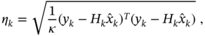
Typical RMSEs produced by the KF and UFIR algorithms versus ![]() are shown in Fig. 6.8 [183], where we recognize several basic features. It can be seen that the KF and UFIR filter modified for CMN give fewer errors than the original ones. It should also be noted that GKF performs better when
are shown in Fig. 6.8 [183], where we recognize several basic features. It can be seen that the KF and UFIR filter modified for CMN give fewer errors than the original ones. It should also be noted that GKF performs better when ![]() , and that the general UFIR filter is more accurate when
, and that the general UFIR filter is more accurate when ![]() . This means that a more robust UFIR filter may be a better choice when measurement noise is heavily colored.
. This means that a more robust UFIR filter may be a better choice when measurement noise is heavily colored.
![Schematic illustration of typical RMSEs produced by KF and UFIR filter for a two-state model versus the coloredness factor Ψ [183].](https://imgdetail.ebookreading.net/2023/10/9781119863076/9781119863076__9781119863076__files__images__c06f008.png)
Figure 6.8 Typical RMSEs produced by KF and UFIR filter for a two‐state model versus the coloredness factor  [183].
6.6.2 Colored Process Noise
Unlike the CMN, which always needs to be filtered out, the CPN, or at least its slow spectral components, can be tracked to avoid losing information about the process behavior. Let us show how to deal with CMN based on the following the state‐space model
where matrices ![]() ,
, ![]() , and
, and ![]() are nonsingular,
are nonsingular, ![]() , and
, and ![]() is the Gauss‐Markov CPN. Noise vectors
is the Gauss‐Markov CPN. Noise vectors ![]() and
and ![]() are mutually uncorrelated with the covariances
are mutually uncorrelated with the covariances ![]() and
and ![]() . The coloredness factor matrix
. The coloredness factor matrix ![]() is chosen such that the CPN
is chosen such that the CPN ![]() is always stationary.
is always stationary.
Using state differencing (3.175a), a new state equation can be written as
where ![]() is white Gaussian,
is white Gaussian, ![]() ,
, ![]() , and
, and ![]() is defined by solving for initial
is defined by solving for initial ![]() the NARE
the NARE ![]() , where
, where ![]() .
.
Using (3.188), we write the modified observation equation as
where ![]() can be substituted with the available past estimate
can be substituted with the available past estimate ![]() .
.
The pseudocode of the UFIR algorithm developed for CPN is listed as Algorithm 14. To initialize iterations, Algorithm 14 employs a short data vector ![]() and an auxiliary matrix
and an auxiliary matrix

Note that, by setting ![]() and
and ![]() , Algorithm 14 becomes the standard iterative UFIR filtering algorithm.
, Algorithm 14 becomes the standard iterative UFIR filtering algorithm.
The error covariance of the UFIR filter modified for CPN can be found if we notice that ![]() , where
, where ![]() . Since this estimate is subject to the constraint
. Since this estimate is subject to the constraint ![]() [182], the error
[182], the error ![]() for
for ![]() can be transformed to
can be transformed to

and the corresponding error covariance ![]() found to be
found to be
This finally gives
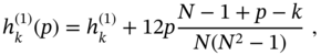
Typical RMSEs produced by the modified and original filters for a two‐state polynomial model with CPN are shown in Fig. 6.9 as functions of the scalar coloredness factor ![]() [182]. The filtering effect here is reminiscent of the effect shown in Fig. 6.6 for CMN, and we notice that the accuracy of the original filters has been improved. However, a significant improvement in performance is recognized only when the coloredness factor is relatively large,
[182]. The filtering effect here is reminiscent of the effect shown in Fig. 6.6 for CMN, and we notice that the accuracy of the original filters has been improved. However, a significant improvement in performance is recognized only when the coloredness factor is relatively large, ![]() . Otherwise, the discrepancies between the filter outputs are not significant.
. Otherwise, the discrepancies between the filter outputs are not significant.
![Schematic illustration of typical RMSEs produced by the two-state UFIR filter, KF, and modified KF and UFIR filter in the presence of CPN as functions of the coloredness factor θ [182].](https://imgdetail.ebookreading.net/2023/10/9781119863076/9781119863076__9781119863076__files__images__c06f009.png)
Figure 6.9 Typical RMSEs produced by the two‐state UFIR filter, KF, and modified KF and UFIR filter in the presence of CPN as functions of the coloredness factor  [182].
Considering the previous modifications of the UFIR filter, we finally conclude that the filtering effect in the presence of CMN and/or CPN is noticeable only with strong coloration.
6.7 Extended UFIR Filtering
Representation of physical processes and approximation of systems using linear models does not always fit with practical needs. Looking at the nonlinear model in (3.226) and (3.227) and analyzing the Taylor series approach that results in the extended KF algorithms, we conclude that UFIR filtering can also be adapted to nonlinear behaviors [178], as will be shown next.
Given a nonlinear state‐space model
where ![]() and
and ![]() are mutually uncorrelated, zero mean, and not obligatorily Gaussian additive noise vectors. In Chapter, when derived EKF, it was shown that (6.156) and (6.157) can be approximated using the second‐order Taylor series expansion as
are mutually uncorrelated, zero mean, and not obligatorily Gaussian additive noise vectors. In Chapter, when derived EKF, it was shown that (6.156) and (6.157) can be approximated using the second‐order Taylor series expansion as
where ![]() is the modified observation vector and
is the modified observation vector and ![]() and
and ![]() represent the components resulting from the linearization,
represent the components resulting from the linearization,
in which  ,
,  , and
, and ![]() and
and ![]() are Cartesian basis vectors with the
are Cartesian basis vectors with the ![]() th and
th and ![]() th components unity, and all others are zeros. The nonlinear functions are represented by
th components unity, and all others are zeros. The nonlinear functions are represented by

where ![]() and
and ![]() are Jacobian matrices and
are Jacobian matrices and ![]() and
and  are Hessian matrices.
Based on (6.158) and (6.159), we can now develop the first‐ and second‐order extended UFIR filtering algorithms. Similarly to the EKF‐1 and EKF‐2 algorithms, we will refer to the extended UFIR algorithms as EFIR‐1 and EFIR‐2.
6.7.1 First‐Order Extended UFIR Filter
Let us look at the model in (6.158) and (6.159) again and assume that the mutually uncorrelated ![]() and
and ![]() are zero mean and white Gaussian. The EFIR‐1 (first‐order) filtering algorithm can be designed using the following recursions [178]
are zero mean and white Gaussian. The EFIR‐1 (first‐order) filtering algorithm can be designed using the following recursions [178]
The pseudocode of the EFIR‐1 filtering algorithm is listed as Algorithm 15. As in the EKF‐1 algorithm, here the prior estimate ![]() is obtained using a nonlinear projection
is obtained using a nonlinear projection ![]() , and then
, and then ![]() is projected onto the observation as
is projected onto the observation as ![]() . Also, the system and observation matrices
. Also, the system and observation matrices ![]() and
and ![]() are Jacobian. The error covariance for this filter can be computed using (6.37) and the Jacobian matrices
are Jacobian. The error covariance for this filter can be computed using (6.37) and the Jacobian matrices ![]() and
and ![]() .
.
The EFIR‐1 filtering algorithm developed in this way turns out to be simple and in most cases truly efficient. However, it should be noted that the initial state ![]() , computed linearly in line 5 of Algorithm 15, may be too rough when the nonlinearity is strong. If so, then
, computed linearly in line 5 of Algorithm 15, may be too rough when the nonlinearity is strong. If so, then ![]() can be computed using multiple projections as
can be computed using multiple projections as ![]() ,
, ![]() , ...,
, ..., ![]() . Otherwise, an auxiliary EKF‐1 algorithm can be used to obtain
. Otherwise, an auxiliary EKF‐1 algorithm can be used to obtain ![]() .
.
6.7.2 Second‐Order Extended UFIR Filter
The derivation of the second‐order EFIR‐2 filter is more complex, and its application may not be very useful because it loses the ability to ignore noise covariances. To come up with the EFIR‐2 algorithm, we will mainly follow the results obtained in [178].
We first define the prior estimate by
for which, by the cyclic property of the trace operator, the expectation of ![]() can be found as
can be found as

We can show that for ![]() given by (6.164), the expectation of the prior error
given by (6.164), the expectation of the prior error ![]() becomes identically zero,
becomes identically zero,
Averaging the nonlinear function ![]() gives
gives
where the expectation of ![]() can be found as
can be found as

that allows us to obtain the error covariance as will be shown next.
Prior Error Covariance
Using (6.158) and (6.164) and taking into account that, for zero mean Gaussian noise, the vector ![]() and other similar vectors are equal to zero, the a priori error covariance
and other similar vectors are equal to zero, the a priori error covariance ![]() can be transformed as
can be transformed as

where matrix ![]() is specialized via its
is specialized via its ![]() th component
th component

Posterior Error Covariance
Reasoning similarly, the a posteriori error covariance ![]() can be transformed using extended nonlinearities if we first represent it as
can be transformed using extended nonlinearities if we first represent it as

take into account that ![]() and
and ![]() , provide the averaging, and obtain
, provide the averaging, and obtain

Due to the symmetry of the matrices ![]() ,
, ![]() , and
, and ![]() , the following expectations can be transformed as
, the following expectations can be transformed as

Then, taking into account that the expectations of other products are matrices with zero components, we finally write the covariance ![]() in the form
in the form

where, the ![]() th component of matrix
th component of matrix ![]() is defined by
is defined by
and the ![]() th component of matrix
th component of matrix ![]() is
is

It has to be remarked now that when developing the second‐order extended algorithms, the authors use two forms of ![]() . The complete form in (6.170) can be found in [12,157]. On the contrary, in [72,185] only first‐order components are preserved.
. The complete form in (6.170) can be found in [12,157]. On the contrary, in [72,185] only first‐order components are preserved.
The pseudocode of the EFIR‐2 filtering algorithm is listed as Algorithm 16. For the given ![]() ,
, ![]() , and
, and ![]() , the set of auxiliary matrices is computed and updated at each
, the set of auxiliary matrices is computed and updated at each ![]() . Then all matrices and vectors are updated iteratively, and the last updated
. Then all matrices and vectors are updated iteratively, and the last updated ![]() and
and ![]() go to the output when
go to the output when ![]() . Although the second‐order EFIR‐2 algorithm has been designed to improve accuracy, empirical studies show that its usefulness is questionable due to the following drawbacks:
. Although the second‐order EFIR‐2 algorithm has been designed to improve accuracy, empirical studies show that its usefulness is questionable due to the following drawbacks:
- Unlike the EFIR‐1 Algorithm 15, the EFIR‐2 Algorithm 16 requires
 and
and  and is thus less robust. It thus has more in common with the EKF rather than with the EFIR‐1 filter.
 - As noted in [178], nothing definite can be said about the accuracy of the EFIR‐2 algorithm compared to the EFIR‐1 algorithm. The same conclusion was made earlier in [185] regarding the EKF‐2 algorithm.
Overall, it can be said that the EFIR‐2 and EKF‐2 filtering algorithms do not demonstrate essential advantages over the EFIR‐1 and EKF‐1 algorithms. Moreover, these algorithms are more computationally complex and slower in operation.
6.8 Robustness of the UFIR Filter
Practice dictates that having a good estimator is not enough if the operating conditions are not satisfied from various perspectives, especially in unknown environments. In such a case, the required estimator must also be robust. In Chapter, we introduced the fundamentals of robustness, which is seen as the ability of an estimator not to respond to undesirable factors such as errors in noise statistics, model errors, and temporary uncertainties. We are now interested in investigating the trade‐off in robustness between the UFIR estimator and some other available state estimators. To obtain reliable results, we will examine along the KF, which is optimal and not robust, and the robust game theory recursive ![]() filter (3.307)–(3.310), which was developed in [185]. We will use the following state‐space model
filter (3.307)–(3.310), which was developed in [185]. We will use the following state‐space model
where the noise covariances ![]() and
and ![]() in the noise vectors
in the noise vectors ![]() and
and ![]() are not necessarily known, as required by KF. To apply the
are not necessarily known, as required by KF. To apply the ![]() filter,
filter, ![]() and
and ![]() will be thought of as norm‐bounded with symmetric and positive definite matrices
will be thought of as norm‐bounded with symmetric and positive definite matrices ![]() and
and ![]() .
.
In our scenario, there is not enough information about ![]() and
and ![]() to optimally tune KF, and the maximum values of the matrices
to optimally tune KF, and the maximum values of the matrices ![]() and
and ![]() are also not known to make the
are also not known to make the ![]() filter robust. Therefore, we organize a scaling test for robustness by representing any uncertain component
filter robust. Therefore, we organize a scaling test for robustness by representing any uncertain component ![]() in (6.173) and (6.174) as
in (6.173) and (6.174) as ![]() , where the increment
, where the increment ![]() is due to a positive‐valued scaling factor
is due to a positive‐valued scaling factor ![]() such that
such that ![]() means undisturbed
means undisturbed ![]() . This test can be applied with the following substitutions:
. This test can be applied with the following substitutions: ![]() ,
, ![]() ,
, ![]() ,
, ![]() ,
, ![]() , and
, and ![]() , where the set of scaling factors
, where the set of scaling factors ![]() can either change matrices or not when
can either change matrices or not when ![]() . For
. For ![]() , the product matrix
, the product matrix ![]() becomes
becomes

We can learn about the robustness of recursive estimators by examining the sensitivity of the bias correction gain to interfering factors and its immunity to these factors. Taken from the UFIR Algorithm 11, the alternate KF (3.92)–(3.96) [184], and the ![]() filter (3.307)–(3.310) [185], the bias corrections gains can be written as, respectively,
filter (3.307)–(3.310) [185], the bias corrections gains can be written as, respectively,
where ![]() ,
, ![]() , and matrix
, and matrix ![]() is constrained by the positive definite matrix
is constrained by the positive definite matrix ![]() . Note that the tuning factor
. Note that the tuning factor ![]() is required by the game theory
is required by the game theory ![]() filter in order to outperform KF.
filter in order to outperform KF.
The influence of ![]() on (6.176)–(6.178) can be learned if we use the following rule: if the error factor causes a decrease in
on (6.176)–(6.178) can be learned if we use the following rule: if the error factor causes a decrease in ![]() , then the bias errors will grow; otherwise, random errors will dominate. The increments
, then the bias errors will grow; otherwise, random errors will dominate. The increments ![]() caused by the error factors in the bias correction gains can now be represented for each of the filters as
caused by the error factors in the bias correction gains can now be represented for each of the filters as

and we notice that lower ![]() means higher robustness. There is one more important preliminary remark to be made. While more tuning factors make an estimator potentially more accurate and precise, it also makes an estimator less robust due to possible tuning errors (Fig. 1.3). In this sense, the two‐parameter
means higher robustness. There is one more important preliminary remark to be made. While more tuning factors make an estimator potentially more accurate and precise, it also makes an estimator less robust due to possible tuning errors (Fig. 1.3). In this sense, the two‐parameter ![]() UFIR filter appears to be more robust, but less accurate, while the four‐parameter
UFIR filter appears to be more robust, but less accurate, while the four‐parameter ![]() KF and five‐parameter
KF and five‐parameter ![]() game theory
game theory ![]() filter are less robust but potentially more accurate.
filter are less robust but potentially more accurate.
6.8.1 Errors in Noise Covariances and Weighted Matrices
The additional errors produced by estimators applied to stochastic models and caused by ![]() and
and ![]() occur due to the practical inability to collect accurate estimates of noise covariances and norm‐bounded weights, especially for LTV systems.
occur due to the practical inability to collect accurate estimates of noise covariances and norm‐bounded weights, especially for LTV systems.
UFIR Filter
The UFIR filter does not require any information about zero mean noise. Thus, this filter is insensitive (robust) to variations in ![]() and
and ![]() , unlike the KF and game theory
, unlike the KF and game theory ![]() filter.
filter.
Kalman Filter
For ![]() and
and ![]() , errors in the KF can be learned in stationary mode if we allow
, errors in the KF can be learned in stationary mode if we allow ![]() . Accordingly, the error covariance can be represented using the DARE
. Accordingly, the error covariance can be represented using the DARE

The solution to (6.179) does not exist in simple form. But if we accept ![]() , which is true for low measurement noise,
, which is true for low measurement noise, ![]() , then (6.179) can be replaced by the discrete Lyapunov equation [184] (A.34)
, then (6.179) can be replaced by the discrete Lyapunov equation [184] (A.34)
which is solvable (A.35). Although approximation (6.180) can be rough when ![]() is not small, it helps to compare the KF and
is not small, it helps to compare the KF and ![]() filter for robustness, as will be shown next.
filter for robustness, as will be shown next.
When ![]() , we can assume that KF is tracking state with high precision and let
, we can assume that KF is tracking state with high precision and let ![]() that gives
that gives ![]() . This gives
. This gives ![]() and
and ![]() , and we conclude that
, and we conclude that ![]() . Note that this relationship is consistent with the equality in (6.183), which was obtained for the isolated cases of
. Note that this relationship is consistent with the equality in (6.183), which was obtained for the isolated cases of ![]() and
and ![]() .
.
Referring to lemma 6.1, the bias correction gain (6.177) can now be approximated for ![]() by the inequality
by the inequality

which does not hold true for ![]() . It is worth noting that
. It is worth noting that ![]() and
and ![]() act in opposite directions, and therefore the worst case will be when
act in opposite directions, and therefore the worst case will be when ![]() and
and ![]() or vice versa.
or vice versa.
Game Theory  Filter
Reasoning similarly for equal weighting errors obtained with ![]() , the bias correction gain (6.178) for the recursive game theory
, the bias correction gain (6.178) for the recursive game theory ![]() filter can be approximated by the inequality [180]
filter can be approximated by the inequality [180]

It can be seen that ![]() makes no difference with the KF gain (6.184) for Gaussian models implying
makes no difference with the KF gain (6.184) for Gaussian models implying ![]() and
and ![]() . Otherwise, we can expect KF to be less accurate and the
. Otherwise, we can expect KF to be less accurate and the ![]() filter to perform better, provided that both
filter to perform better, provided that both ![]() and
and ![]() are properly maximized. Indeed, if we assume that
are properly maximized. Indeed, if we assume that ![]() and
and ![]() , then we can try to find some small
, then we can try to find some small ![]() such that the effect of
such that the effect of ![]() and
and ![]() is compensated. However, if
is compensated. However, if ![]() is not set properly, the
is not set properly, the ![]() filter can cause even more errors than the KF. Moreover, even if
filter can cause even more errors than the KF. Moreover, even if ![]() is set properly, any deviation of
is set properly, any deviation of ![]() from unity will additionally chance the gain through the product of
from unity will additionally chance the gain through the product of ![]() . More information and examples on this topic can be found in [180].
. More information and examples on this topic can be found in [180].
What follows behind the approximations (6.184) and (6.185) is that, if properly tuned with ![]() , the
, the ![]() filter will be more accurate than the KF in the presence of errors in noise covariances. In practice, however, it can be difficult to find and set the correct
filter will be more accurate than the KF in the presence of errors in noise covariances. In practice, however, it can be difficult to find and set the correct ![]() , especially for LTV systems that imply a new
, especially for LTV systems that imply a new ![]() at each point in time. If so, then the
at each point in time. If so, then the ![]() filter may give more errors and even diverge. Thus, the relationship between the filters in terms of robustness to errors in noise statistics should be practically as follows:
filter may give more errors and even diverge. Thus, the relationship between the filters in terms of robustness to errors in noise statistics should be practically as follows:
where ![]() holds true for properly maximized
holds true for properly maximized ![]() and
and ![]() and properly set
and properly set ![]() . Otherwise, the KF may perform better. In turn, the UFIR filter that is
. Otherwise, the KF may perform better. In turn, the UFIR filter that is ![]() ‐invariant may be a better choice, especially with large errors in noise covariances.
‐invariant may be a better choice, especially with large errors in noise covariances.
6.8.2 Model Errors
Permanent estimation errors arise from incorrect modeling and persistent model uncertainties, known as mismodeling, when the model is not fully consistent with the process over all time [69]. If no improvement is expected in the model, then the best choice may be to use robust estimators, in which case testing becomes an important subject of confirmation of the estimator accuracy and stability.
UFIR Filter
In UFIR filtering, errors caused by ![]() are taken into account only on the horizon
are taken into account only on the horizon ![]() . Accordingly, the bias correction gain
. Accordingly, the bias correction gain ![]() can be expressed as
can be expressed as

and approximated using the following lemma.
The gain ![]() can finally be approximated with
can finally be approximated with


It is seen that the factor ![]() affects
affects ![]() directly and as a reciprocal. However, the same cannot be said about the factor
directly and as a reciprocal. However, the same cannot be said about the factor ![]() raised to the power
raised to the power ![]() . Indeed, for
. Indeed, for ![]() , the gain
, the gain ![]() can significantly grow. Otherwise, when
can significantly grow. Otherwise, when ![]() , it decreases. Thus, we conclude that the effect of errors in the system matrix on the bias correction gain of the UFIR filter is more complex than the effect of errors in the observation matrix.
, it decreases. Thus, we conclude that the effect of errors in the system matrix on the bias correction gain of the UFIR filter is more complex than the effect of errors in the observation matrix.
Kalman Filter
When examining Kalman filter errors associated with mismodeling, ![]() and
and ![]() , it should be kept in mind that such errors are usually observed along with errors in noise covariances. If we ignore errors in the description of noise, the picture will be incomplete due to multiplicative effects. Therefore, we assume that
, it should be kept in mind that such errors are usually observed along with errors in noise covariances. If we ignore errors in the description of noise, the picture will be incomplete due to multiplicative effects. Therefore, we assume that ![]() and
and ![]() , and analyze the errors similarly to the UFIR filter. To do this, we start with the discrete Lyapunov equation 6.180, the solution of which can be approximated using the following lemmas.
, and analyze the errors similarly to the UFIR filter. To do this, we start with the discrete Lyapunov equation 6.180, the solution of which can be approximated using the following lemmas.
Referring to lemma 6.3 and lemma 6.4, the bias correction gain ![]() of the KF, which is given by (6.177), can be approximated as
of the KF, which is given by (6.177), can be approximated as

and we notice that inequality (6.196) is inapplicable to some models.
Analyzing (6.195), it can be concluded that the mismodeling errors, ![]() , and errors in noise covariance,
, and errors in noise covariance, ![]() , cause multiplicative effects in the Kalman gain. In the best case, these effects can compensate for each another, although not completely. In the worst case, which is of practical interest, errors can grow essentially. Again, we see that
, cause multiplicative effects in the Kalman gain. In the best case, these effects can compensate for each another, although not completely. In the worst case, which is of practical interest, errors can grow essentially. Again, we see that ![]() and
and ![]() act in opposite directions, as in the case of
act in opposite directions, as in the case of ![]() .
.
Game Theory  Filter
The game theory ![]() filter obtained in [185] does not take into account errors in the system and observation matrices. Therefore, it is interesting to know its robustness to such errors in comparison with the UFIR filter and KF. Referring to (6.195) and (6.196), the bias correction gain
filter obtained in [185] does not take into account errors in the system and observation matrices. Therefore, it is interesting to know its robustness to such errors in comparison with the UFIR filter and KF. Referring to (6.195) and (6.196), the bias correction gain ![]() of the
of the ![]() filter, which is given by (6.178), can be approximated for
filter, which is given by (6.178), can be approximated for ![]() and
and ![]() by
by


These inequalities more clearly demonstrate the key advantage of the ![]() filter: a properly set
filter: a properly set ![]() can dramatically improve the estimation accuracy. Indeed, if the tuning factor
can dramatically improve the estimation accuracy. Indeed, if the tuning factor ![]() constrained by
constrained by ![]() is chosen such that the relationships in parentheses become zero, then it follows that the effects of
is chosen such that the relationships in parentheses become zero, then it follows that the effects of ![]() are reduced to zero, and errors in the observation matrix will remain the main source. Furthermore, by adjusting
are reduced to zero, and errors in the observation matrix will remain the main source. Furthermore, by adjusting ![]() , the effect of
, the effect of ![]() can be fully compensated.
can be fully compensated.
Unfortunately, the previous remedy is effective only if the correct ![]() is available at any given time. Otherwise, the
is available at any given time. Otherwise, the ![]() filter may produce more errors than the KF, and can even diverge. For more information, the reader can read [180], where a complete analysis for robustness is presented with typical examples.
filter may produce more errors than the KF, and can even diverge. For more information, the reader can read [180], where a complete analysis for robustness is presented with typical examples.
The general conclusion that can be drawn from the analysis of the impact of mismodeling errors is that, under ![]() and
and ![]() , the KF performance can degrade dramatically and that the
, the KF performance can degrade dramatically and that the ![]() can improve it if we set a proper tuning factor
can improve it if we set a proper tuning factor ![]() at each time instant. Since this is hardly possible for many practical applications, the UFIR filter is still preferred, and the relationship between the filters in terms of robustness to model errors will generally be the same (6.186), where
at each time instant. Since this is hardly possible for many practical applications, the UFIR filter is still preferred, and the relationship between the filters in terms of robustness to model errors will generally be the same (6.186), where ![]() holds true for properly maximized errors in
holds true for properly maximized errors in ![]() and
and ![]() if
if ![]() and
and ![]() are properly maximized and
are properly maximized and ![]() is set properly. Otherwise, the
is set properly. Otherwise, the ![]() filter may give large errors and go to divergence, while the KF may perform better.
filter may give large errors and go to divergence, while the KF may perform better.
6.8.3 Temporary Uncertainties
Certainly persistent model errors can seriously degrade the estimator performance, causing uncontrollable bias errors. But their effect can be mitigated by improving the model, at least theoretically. What cannot be done efficiently is the elimination of errors caused by temporary uncertainties such as jumps in phase, frequency, and velocity. Such errors are not easy to deal with due to the unpredictability and short duration of the impacts. The problem is complicated by the fact that temporary uncertainties exist in different forms, and it is hard to imagine that they have a universal model.
One way to investigate the associated estimation errors is to assume that the model has no past errors up to the time index ![]() and that the uncertainty caused by
and that the uncertainty caused by ![]() occurs at
occurs at ![]() . The estimator that is less sensitive to such an impact caused by
. The estimator that is less sensitive to such an impact caused by ![]() at
at ![]() can be said to be the most robust.
can be said to be the most robust.
UFIR Filter
Suppose the model is affected by ![]() over all time and that
over all time and that ![]() is known at
is known at ![]() . At the next step, at
. At the next step, at ![]() , the system experiences an unpredictable impact caused by
, the system experiences an unpredictable impact caused by ![]() and
and ![]() . Provided that
. Provided that ![]() is also known at
is also known at ![]() , the bias correction gain
, the bias correction gain ![]() of the UFIR filter (6.176) can be transformed to
of the UFIR filter (6.176) can be transformed to

As can be seen, ![]() and
and ![]() act in the same way in (6.199) as in the case of model errors represented by (6.192). However, the effect in (6.199) turns out to be stronger because of the square of
act in the same way in (6.199) as in the case of model errors represented by (6.192). However, the effect in (6.199) turns out to be stronger because of the square of ![]() , in contrast to (6.192). This means that temporary data errors have a stronger effect on the UFIR filter than permanent model errors. The conclusion just made should not be unexpected, given the fact that rapid changes cause transients, the values of which usually exceed steady‐state errors.
, in contrast to (6.192). This means that temporary data errors have a stronger effect on the UFIR filter than permanent model errors. The conclusion just made should not be unexpected, given the fact that rapid changes cause transients, the values of which usually exceed steady‐state errors.
Kalman Filter
The Kalman gain can be approximated similarly to the bias correction gain of the UFIR filter. Substituting the prior estimate ![]() into (6.177), where the matrices are scaled by the error factors
into (6.177), where the matrices are scaled by the error factors ![]() and
and ![]() taking into account that
taking into account that ![]() , we obtain the approximation of the Kalman gain in the form
, we obtain the approximation of the Kalman gain in the form

Analyzing (6.199) and (6.200), we draw attention to an important feature. Namely, the effect of the first ![]() is partially compensated by the second
is partially compensated by the second ![]() in the parentheses, which is not observed in the UFIR filter. Because of this, the KF responds to temporary uncertainty with lower values than the UFIR filter. In other words, the UFIR filter is more sensitive to temporary uncertainties. On the other hand, all transients in the UFIR filter are limited by
in the parentheses, which is not observed in the UFIR filter. Because of this, the KF responds to temporary uncertainty with lower values than the UFIR filter. In other words, the UFIR filter is more sensitive to temporary uncertainties. On the other hand, all transients in the UFIR filter are limited by ![]() points, while the KF filter generates long transients due to IIR. Both these effects, which are always seen in practice, represent one of the fundamental differences between the UFIR filter and the KF [179].
points, while the KF filter generates long transients due to IIR. Both these effects, which are always seen in practice, represent one of the fundamental differences between the UFIR filter and the KF [179].
Transients in the UFIR filter and KF: Responding to the stepwise temporary uncertainty, the UFIR filter produces
points transient with a larger overshoot, and the KF produces a longer transient with a shorter overshoot.
Examples of transients in the UFIR filter and KF are given in Fig. 4.2 and Fig. 6.3, and we notice that the difference between the overshoots is usually ![]() .
.
Game Theory  Filter
Providing similar transformations as for (6.200), we approximate the bias correction gain of the ![]() filter (6.178) as
filter (6.178) as

and notice an important difference with (6.200). In (6.201), there is an additional term containing ![]() , which can be chosen such that the effect of
, which can be chosen such that the effect of ![]() is fully compensated. This is considered to be the main advantage of the game theory
is fully compensated. This is considered to be the main advantage of the game theory ![]() filter over KF. The drawback is that the tuning factor
filter over KF. The drawback is that the tuning factor ![]() is an unknown analytical function of the set
is an unknown analytical function of the set ![]() , which contains uncertain components. Therefore, if
, which contains uncertain components. Therefore, if ![]() cannot be set properly at every point of time, the
cannot be set properly at every point of time, the ![]() filter performance may significantly degrade, and the filter may even demonstrate the divergence [180]. Analyzing (6.201), it can also be noted that the problem is complicated by the higher sensitivity of
filter performance may significantly degrade, and the filter may even demonstrate the divergence [180]. Analyzing (6.201), it can also be noted that the problem is complicated by the higher sensitivity of ![]() to
to ![]() .
.
All that follows from the previous analysis of estimation errors caused by temporary uncertainties is that the UFIR filter can still be considered the most robust solution. The game theory ![]() filter can improve the performance of KF by properly setting the tuning factor
filter can improve the performance of KF by properly setting the tuning factor ![]() . However, since the exact
. However, since the exact ![]() is not available at every point of time, this filter can become unstable and diverge.
is not available at every point of time, this filter can become unstable and diverge.
6.9 Implementation of Polynomial UFIR Filters
Hardware implementation of digital filters is usually not required in state space. In contrast, scalar input‐to‐output structures have found much more applications. Researchers often prefer to use UFIR polynomial structures, whenever suboptimal filtering is required. Examples can be found in tracking, control, positioning, timekeeping, etc. If such a UFIR filter matches the model, then the group delay reaches a minimum. Otherwise, the group delay grows at a lower rate than in IIR filters. This makes UFIR structures very useful in engineering practice of suboptimal filtering. Next we will present and analyze the polynomial UFIR structures in the ![]() domain [29] and discrete Fourier transform (DFT) domain [30].
domain [29] and discrete Fourier transform (DFT) domain [30].
6.9.1 Filter Structures in  ‐Domain
The transfer function ![]() of the
of the ![]() th degree polynomial UFIR filter is specialized by the
th degree polynomial UFIR filter is specialized by the ![]() ‐transform applied to the FIR function
‐transform applied to the FIR function ![]() given by (6.120) with
given by (6.120) with ![]() ; that is,
; that is,


where ![]() ,
, ![]() is an angular frequency,
is an angular frequency, ![]() is the sampling time,
is the sampling time, ![]() is given by (6.121), and conventionally we will also use
is given by (6.121), and conventionally we will also use ![]() in
in ![]() as the imaginary sign
as the imaginary sign ![]() . The following properties of
. The following properties of ![]() can be listed in addition to the inherent
can be listed in addition to the inherent ![]() ‐periodicity, symmetry of
‐periodicity, symmetry of ![]() , and antisymmetry of
, and antisymmetry of ![]() .
.
- Transfer function at
 . By
. By  , the transfer function becomes
(6.203)for all
, the transfer function becomes
(6.203)for all
 , which means that the UFIR filter is an LP filter.
 - Impulse response at
 . By the inverse
  ‐transform, the value of
  at
at  is defined as
Because
 is always positive‐valued,
  , and for all
  , the counterclockwise circular integration in (6.204a) always produces a positive imaginary value, which gives(6.205)
- Transfer function at
 . By
. By  , the transfer function becomes
(6.206)where
, the transfer function becomes
(6.206)where
 is the Euler polynomial. For low‐degree impulse responses, the Euler polynomials become
  ,
,  ,
,  , and
, and  .
. - Energy. By Parseval's theorem, the following relations hold
(6.207a)
 (6.207b)
and it follows that the energy (or squared norm) of the FIR function in the
 domain is equal to the value of
  at
at  .
. - Unbiasedness in the
 domain. The following theorem establishes an unbiasedness condition that is fundamental to digital FIR filters in the
  domain.
- Noise power gain. The squared norm of
 , which represents the NPG
  of the UFIR filter (Table 6.2), is also the energy of
  . By Parseval's theorem, NPG takes the following equivalent forms
(6.209a)
. By Parseval's theorem, NPG takes the following equivalent forms
(6.209a) (6.209b)
 (6.209c)


It is worth noting that using to the properties listed, it becomes possible to design and optimize polynomial FIR filter structures in the ![]() domain with maximum efficiency for real‐time operation.
domain with maximum efficiency for real‐time operation.
Transfer Function in the  ‐Domain
Although the inner sum in (6.202b) does not have a closed form, the properties of the FIR filter in the ![]() ‐domain allow one to represent
‐domain allow one to represent ![]() as
as

By assigning the following subtransfer functions


the generalized block diagram of the ![]() th degree UFIR filter can be shown as in Fig. 6.10. The low‐degree coefficients
th degree UFIR filter can be shown as in Fig. 6.10. The low‐degree coefficients ![]() ,
, ![]() , and
, and ![]() are listed for this structure in Table 6.3 [29].
are listed for this structure in Table 6.3 [29].
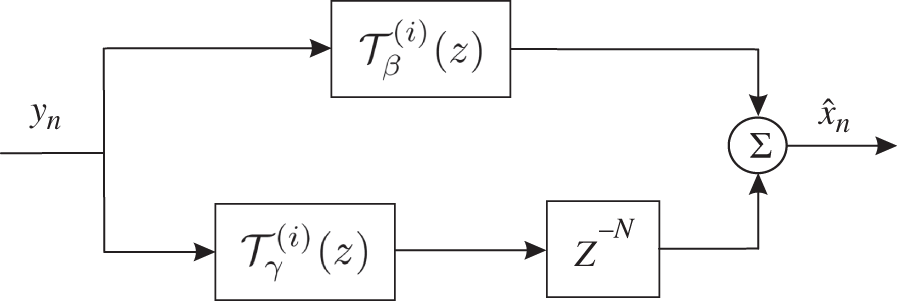
Figure 6.10 Generalized block diagram of the  th degree UFIR filter.
Table 6.3 Coefficients ![]() ,
, ![]() , and
, and ![]() of Low‐Degree UFIR Filters.
of Low‐Degree UFIR Filters.
| 0 | 1 | 2 | 3 | |
|---|---|---|---|---|
| 0 | − | − | − | |
| 0 | 0 | |||
| 0 | 0 | 0 | − | |
| − | − | |||
| 0 | − | − | ||
| 0 | 0 | − | ||
| 0 | 0 | 0 | − | |
| −1 | −2 | −3 | −4 | |
| 0 | 1 | 3 | 6 | |
| 0 | 0 | −1 | −4 | |
| 0 | 0 | 0 | 1 | |
The magnitude response functions ![]() of low‐degree polynomial UFIR filters are shown in Fig. 6.12. A distinctive feature of LP filters of this type is a negative slop of 20 dB per decade in the Bode plot (Fig. 6.12b) in the transient region. Another feature is that increasing the degree of the polynomial filter expands the bandwidth. It can also be seen that the transfer function has multiple intensive side lobes that are related to the shape of the impulse response (Fig. 6.5). The later property is discouraged in the design of standard LP filters. However, it is precisely this shape of
of low‐degree polynomial UFIR filters are shown in Fig. 6.12. A distinctive feature of LP filters of this type is a negative slop of 20 dB per decade in the Bode plot (Fig. 6.12b) in the transient region. Another feature is that increasing the degree of the polynomial filter expands the bandwidth. It can also be seen that the transfer function has multiple intensive side lobes that are related to the shape of the impulse response (Fig. 6.5). The later property is discouraged in the design of standard LP filters. However, it is precisely this shape of ![]() that guarantees the filter unbiasedness.
that guarantees the filter unbiasedness.
Figure 6.12a assures that bias is eliminated at the filter output by shifting and lifting the side lobes of a zero‐degree uniform FIR filter, which provides simple averaging. Accordingly, the ![]() ‐degree filter passes the spectral content close to zero without change, magnifies the components falling into the first lobe, and attenuates the power of the higher‐frequency components with 10 dB per decade (Fig. 6.12b).
‐degree filter passes the spectral content close to zero without change, magnifies the components falling into the first lobe, and attenuates the power of the higher‐frequency components with 10 dB per decade (Fig. 6.12b).
The phase response functions ![]() of low‐degree polynomial UFIR filters are shown in Fig. 6.13a, and the group delay functions obtained by
of low‐degree polynomial UFIR filters are shown in Fig. 6.13a, and the group delay functions obtained by ![]() are shown in Fig. 6.13b. The phase response function of this filter is linear on average (Fig. 6.13a). However, the phase response changes following variations in the magnitude response, which, in turn, leads to changes in the group delay around a small constant value (Fig. 6.13b). From the standpoint of the design of basic LP filters, the presence of periodic variations in the phase response is definitely a disadvantage. But it is also a key condition that cannot be violated without making the filter output biased.
are shown in Fig. 6.13b. The phase response function of this filter is linear on average (Fig. 6.13a). However, the phase response changes following variations in the magnitude response, which, in turn, leads to changes in the group delay around a small constant value (Fig. 6.13b). From the standpoint of the design of basic LP filters, the presence of periodic variations in the phase response is definitely a disadvantage. But it is also a key condition that cannot be violated without making the filter output biased.

Figure 6.13 Phase response functions of the low‐degree UFIR filters for  : (a) phase response
  and (b) group delay
  .
.
6.9.2 Transfer Function in the DFT Domain
The DFT of the ![]() th degree UFIR filter impulse response
th degree UFIR filter impulse response ![]() is obtained as
is obtained as

where ![]() . In addition to the inherent
. In addition to the inherent ![]() ‐periodicity, the symmetry of
‐periodicity, the symmetry of ![]() , and the antisymmetry of
, and the antisymmetry of ![]() , the following properties are important for the implementation of UFIR filters in the DFT domain.
, the following properties are important for the implementation of UFIR filters in the DFT domain.
- DFT value at
 . By
. By  , the function
  becomes unity,
  , and, by the properties listed in Table 6.2, the DFT function (6.214) is transformed to
(6.215)for all
, and, by the properties listed in Table 6.2, the DFT function (6.214) is transformed to
(6.215)for all
 , which fits with LP filtering.
 - Impulse response at
 . For
. For  and
and  , the inverse DFT (IDFT) applied to
  gives
(6.216)
gives
(6.216)
Since
 holds for all
  , the sum of the DFT coefficients is real and positive. It then follows that(6.217)
- DFT value at
 . At the point of symmetry
  for even
  , the function
  becomes
  and the following relation holds
(6.218)where
and the following relation holds
(6.218)where
 is the Euler polynomial. For low degrees, the Euler polynomials take the following form:
  ,
,  ,
,  , and
, and  .
. - Noise power gain. As a measure of noise reduction at the UFIR filter output, NPG
 for white Gaussian noise is determined by the energy of
  . The NPG has the following equivalent forms in the DFT domain:
(6.219a)
. The NPG has the following equivalent forms in the DFT domain:
(6.219a) (6.219b)
 (6.219c)
- Unbiasedness condition in the DFT domain. The following theorem establishes an unbiasedness condition that is fundamental to UFIR filters in the DFT domain.
Proof. To prove (6.220), use the following fundamental condition for optimal filtering: the order of the optimal and/or unbiased filter must be the same as that of the system. Then represent
 by (6.124),
where the coefficient
 is given by (6.125). Recall that function (6.124) has the following main properties, given in Table 6.2: the sum of its coefficients is equal to unity, and the moments zero; that is,(6.221)
 (6.222)
Use Parseval's theorem and obtain the following relationships,
(6.223a) (6.223b)
 (6.223c)
Now observe that the IDFT applied to
 at
at  gives
gives  that finally leads to (6.220) and completes the proof.
 - Estimation error boundary. The concept of NPG
 can be used to specify the bound
  for the estimation error in the three‐sigma sense as
(6.224)where
for the estimation error in the three‐sigma sense as
(6.224)where
 is the standard deviation of the measurement white noise
  .
.
Note that the previously discussed properties of polynomial UFIR filters in the DFT domain are preserved for any polynomial degree, but in practice only low‐degree digital UFIR filters, ![]() , are usually found. The reason for using low‐degree filters is explained earlier: increasing the degree leads to larger random errors at the filter output.
, are usually found. The reason for using low‐degree filters is explained earlier: increasing the degree leads to larger random errors at the filter output.
Transfer Function in the DFT Domain
Using the properties listed, the transfer function ![]() of the
of the ![]() th degree UFIR filter can be represented in the DFT domain with the sum
th degree UFIR filter can be represented in the DFT domain with the sum

in which the inner sum has no closed‐form solution for an arbitrary ![]() . However, solutions can be found for low‐degree polynomials as shown in [30]. Next we will illustrate such a solution for a first‐degree UFIR filter and postpone to “Problems” the search for solutions associated with higher degrees.
. However, solutions can be found for low‐degree polynomials as shown in [30]. Next we will illustrate such a solution for a first‐degree UFIR filter and postpone to “Problems” the search for solutions associated with higher degrees.
The magnitude response ![]() , Bode plot, and phase response
, Bode plot, and phase response ![]() functions of the
functions of the ![]() th degree,
th degree, ![]() , polynomial UFIR filter are shown in Fig. 6.14. For the 1st degree, the functions are computed by (6.226b) and for the next two low degrees the transfer functions can be found in [30]. In addition to the inherent properties of periodicity with a repetition period of
, polynomial UFIR filter are shown in Fig. 6.14. For the 1st degree, the functions are computed by (6.226b) and for the next two low degrees the transfer functions can be found in [30]. In addition to the inherent properties of periodicity with a repetition period of ![]() points, symmetry of
points, symmetry of ![]() , and antisymmetry of
, and antisymmetry of ![]() , the transfer function
, the transfer function ![]() has several other features that are of practical importance.
has several other features that are of practical importance.
- The magnitude response
 is a monotonically decreasing function of
  , which changes from
  to
to  (Fig. 6.14a), and has a transition slope
  on the Bode plot (Fig. 6.14b). So we have further proof that the UFIR filter is essentially an LP filter.
 - The phase response
 is an antisymmetric function existing from
  to
to  on
on  with a positive slope, except for the transient region where an increase in the filter degree makes it more complex (Fig. 6.14c). This function is close to linear for low‐degree filters, and it is strictly linear for the first‐degree filter.

Figure 6.14 DFT of the low‐degree polynomial UFIR filters: (a) magnitude response  for
for  , (b) Bode plot of
  for
for  , and (c) phase response
  for
for  .
.
Finally, we come to an important practical conclusion. Since the transfer function of the polynomial UFIR filter is monotonic and does not contain the periodic variations observed in the ![]() ‐domain (Fig. 6.13), it follows that the filter can be easily implemented with all of the advantages of suboptimal unbiased filtering.
‐domain (Fig. 6.13), it follows that the filter can be easily implemented with all of the advantages of suboptimal unbiased filtering.
6.10 Summary
By abandoning the requirement for initial values and ignoring zero mean noise, the UFIR state estimator appears to be the most robust among other linear estimators such as OFIR, OUFIR, and ML state estimators. Moreover, its iterative algorithm is more robust than the recursive KF algorithm. The only tuning factor required for the UFIR filter is the optimal horizon, which can be determined much more easily than noise statistics. Furthermore, at given averaging horizons, the UFIR state estimator becomes blind, which is very much appreciated in practice. In general, it is only within a narrow range of error factors caused by various types of uncertainties that optimal and ML estimators are superior to the UFIR estimator. For the most part, this explains the better performance of the UFIR state estimator in many real‐world applications.
Like other FIR filters, the UFIR filter operates on the averaging horizon ![]() of
of ![]() points, from
points, from ![]() to
to ![]() . Its discrete convolution‐based batch resembles the LS estimator. But, the latter is not a state estimator. The main performance characteristic of a scalar input‐to‐output UFIR filter is NPG. If the UFIR filter is designed to work in state space, then its noise reduction properties are characterized by GNPG.
. Its discrete convolution‐based batch resembles the LS estimator. But, the latter is not a state estimator. The main performance characteristic of a scalar input‐to‐output UFIR filter is NPG. If the UFIR filter is designed to work in state space, then its noise reduction properties are characterized by GNPG.
The recursive forms used to iteratively compute the batch UFIR estimate are not Kalman recursions. An important feature is that UFIR filter recursions serve any zero mean noise, while Kalman recursions are optimal only for white Gaussian noise. It is worth noting that the error covariance of the UFIR and Kalman filters are represented by the same Riccati equation. The difference lies in the different bias correction gains. The optimal bias correction gain of the KF is called the Kalman gain ![]() , while the bias correction gain of the UFIR filter is computed in terms of GNPG as
, while the bias correction gain of the UFIR filter is computed in terms of GNPG as ![]() .
.
Since the UFIR filter does not involve noise covariances to the algorithm, it minimizes the MSE on the optimal horizon of ![]() points (Fig. 6.1). The significance of
points (Fig. 6.1). The significance of ![]() is that random errors increase if the horizon length
is that random errors increase if the horizon length ![]() is chosen such that
is chosen such that ![]() . Otherwise, bias errors grow if
. Otherwise, bias errors grow if ![]() . Using (6.49), the optimal horizon
. Using (6.49), the optimal horizon ![]() can be estimated through the measurement residual without using ground truth. In response to stepwise temporary uncertainties, the UFIR filter generates finite time transients at
can be estimated through the measurement residual without using ground truth. In response to stepwise temporary uncertainties, the UFIR filter generates finite time transients at ![]() points with larger overshoots, while the KF generates longer transients with lower overshoots. This property represents the main difference between the transients in both filters.
points with larger overshoots, while the KF generates longer transients with lower overshoots. This property represents the main difference between the transients in both filters.
It turns out that, since zero mean noise is ignored by UFIR state estimators, the FFFM, FFBM, BFFM, and BFBM ![]() ‐lag UFIR smoothing algorithms are equivalent. It should also be kept in mind that all unbiased, optimal, and optimal unbiased state estimators are essentially LP filters. Moreover, the zero‐degree (simple average) UFIR filter is the best in the sense of the minimum produces noise. This is because an increase in the filter degree or the number of the states leads to an increase in random errors at the estimator output. It also follows that the set of degree polynomial impulse responses of the UFIR filter establishes a class of discrete orthogonal polynomials that are suitable for signal analysis and restoration due to the built‐in unbiasedness.
‐lag UFIR smoothing algorithms are equivalent. It should also be kept in mind that all unbiased, optimal, and optimal unbiased state estimators are essentially LP filters. Moreover, the zero‐degree (simple average) UFIR filter is the best in the sense of the minimum produces noise. This is because an increase in the filter degree or the number of the states leads to an increase in random errors at the estimator output. It also follows that the set of degree polynomial impulse responses of the UFIR filter establishes a class of discrete orthogonal polynomials that are suitable for signal analysis and restoration due to the built‐in unbiasedness.
Although the UFIR filter ignores zero mean noise, it is not suitable for colored noise that is biased on short horizons. If the colored noise is well‐approximated by the Gauss‐Markov process, then the general UFIR filter becomes universal for time‐correlated and uncorrelated driving white noise sources. Like GKF, a general UFIR filter can be designed to work with CMN and CPN. It can also be applied to state‐space models with smooth nonlinearities using the first‐ or second‐order Taylor series expansions. However, it turns out that the second‐order EFIR‐2 filter has no practical advantage over the first‐order EFIR‐1 filter.
The implementation of polynomial UFIR filters can be most efficiently obtained in the DFT domain due to the following critical property: the DFT transfer function is smooth and does not exhibit periodic variations inherent to the ![]() ‐domain.
‐domain.
6.11 Problems
- Explain the difference between polynomial fitting and filtering (smoothing) of polynomial models.
- NPG for scalar signals is given by (6.15). Give the interpretation of GNPG defined by (6.16a) for state vectors. Why does the NPG decrease with an increase in the averaging horizon?
- Solved problem: Recursive forms for UFIR filter. Consider the batch UFIR filtering estimate
 with the fundamental gain given by (6.10b). Another way to obtain recursive forms for this filter (Algorithm 11) is the following [179]. Represent the inverse of the GNPG
  as
as

Since
 holds for
  , write
  as
as
substitute to the previous relation, and arrive at the recursion (6.21) for
 .
.Similarly, represent the product
 as
as
combine with
 , obtain
  , substitute
  , and come up with
From (6.21) find
 , substitute into the previous relation, and arrive at the recursion (6.29) for the UFIR estimate.
 - The error covariance of the UFIR filter is given by (6.37) as

Compare this relation to the error covariance of the KF and explain the difference between the bias correction gain
 of the UFIR filter and the Kalman gain
  . Why can the Kalman gain not be less than the optimal value? Why does the bias correction gain
  of the UFIR decrease with increasing the horizon length?
 - To minimize MSE, the averaging horizon for the UFIR filter should be optimal
 (Fig. 6.1) by solving the following minimization problem

Why does the OFIR filter not need an optimal horizon? Why does the error in the OFIR filter decrease with increasing the horizon length, while the UFIR filter minimizes the MSE by only
 ? Give simple and intuitive explanations.
 - Measurement data transmitted over a wireless communication channel with latency are represented at the receiver with the following state‐space equations

where
 ,
,  , is a deterministic weight, which can be either unity or zero. The time‐stamped data indicate a value of
  for which the weight is unity and the other weights are zero. Transform the model to another without delay and develop a UFIR filter.
 - A useful property of the measurement residual
 of the UFIR filter is that the derivative of its trace with respect to the horizon length reaches a minimum when
  approaches
  (Fig. 6.2). This makes it possible to determine
  by (6.49) or by solving the minimization problem

Give an explanation to this fact and discuss the problems that may arise in the practical implementations of this method.
- An open and challenging problem is to find an analytical relationship between
 and noise covariances
  and
and  similarly to (6.51) [153]. Find a solution to this problem for a periodical process observed as

where
 and
and  ,
,  , and
, and  are state variables. Write the state equation with additive white Gaussian noise.
 - The GNPG of the backward UFIR filter is defined by (6.62) as

Represent GNPG as
 and specify
  .
. - The error covariance
 of the backward UFIR filter is given by

Reasoning similarly as for the forward UFIR filter, provide the derivation of (6.72). Analyze this relationship and find out what will happen to
 if the noise covariance
  is set equal to zero.
 - The error covariance of the batch
 ‐lag FFFM UFIR smoother is given by (6.85). Recursive computation of (6.85) is provided by (6.94), where the matrix
  still has a batch form (6.92) given by

Find a recursive form for (6.92) or, otherwise, develop a different approach for recursive computation of (6.85).
- Using deductive reasoning, the recursive form for
 was found as (6.90) and for
  as (6.93), respectively,

Show other possible ways to obtain recursions for (6.90) and (6.93).
- Referring to the optimal state estimation problem and considering the transform of the UFIR filter gain
 , find an explanation for the fact that the optimal, optimal unbiased, ML, and unbiased FIR filters are LP filters.
 - It follows from (6.129) that polynomial FIR functions
 ,
,  , given by (6.124), establish a new class discrete orthogonal polynomials related by the recurrence relation (6.128). Reasoning in a similar way, examine for orthogonality the class of more general
  ‐shift FIR functions
  ,
,  ,
,  , given by (6.120), and find the recurrence relation, if any.
 - Find an explanation for the fact that increasing the number of states makes the state estimator less effective in terms of noise reduction. In this sense, explain why simple averaging is best in terms of the minimum produced noise.
- It follows from Fig. 6.5 that prediction errors grow with increasing the
 ‐step. Which method is more efficient in predicting future states: stochastic prediction requiring future noise values? Deterministic prediction ignoring future noise? Or linear deterministic prediction?
 - General UFIR and Kalman filters serve for correlated and de‐correlated Gauss‐Markov process noise
 and measurement noise
  , where
  and
and  . Can we modify the UFIR filter and KF for non‐Gaussian colored noise? If not, explain why.
 - The periodic system is represented in state space by the equations

where
 is a constant angular measure, and
  and
and  are zero mean noise sources. Using the derivation of the UFIR filter for polynomial models, derive the scalar FIR functions for the first state
  and the second state
  to satisfy the unbiasedness condition
  .
. - The bias correction gain of the KF is approximated by (6.184). Referring to the derivation of (6.184), give a proof of the corresponding approximation (6.185) for the
 filter.
 - Lemma 6.3 states that the prior error covariance
 of the KF is approximated by

where
 and
and  are given constants. Using the proof of lemma 6.1, give a corresponding proof of the lemma 6.3.
 - Using the derivation procedure given in [180], provide a proof of approximation (6.194) of the prior error covariance
 of the KF stated by lemma 6.4.
 - A linear digital system operates normally without uncertainties from the past to the time index
 inclusive. Then it experiences uncertainties in the coefficients
  and
and  at the time index
  . Check that the approximate gains of the UFIR filter (6.199), KF (6.200), and
  filter (6.201) are correct.
 - For the
 th degree polynomial scalar FIR function
  existing on
  and the transfer function
  , the unbiasedness constraint in the
  ‐domain is established by theorem 6.2 as

Obtain the corresponding constraint for the general UFIR filter matrix gain case
 .
. - Given a digital UFIR filter with the
 th degree transfer function
  corresponding to a polynomial FIR function
  existing on
  , theorem 6.3 establishes the unique unbiasedness constrain for this filter in the DFT domain as

Obtain the corresponding constraint for the UFIR filter matrix gain
 .
. - The transfer function
 of the
  th degree polynomial UFIR filter is given in the
  ‐domain by (6.210), which for arbitrary
  has no closed‐form solution. Using the properties of the UFIR filters in the
  ‐domain and Table 6.3, find the closed forms of this function for the second and third degrees and represent the filter with block diagrams similar to that shown in Fig. 6.11.
 - The transfer function
 of the
  th degree polynomial UFIR filter is given by (6.225) and has no closed‐form solution. Find solutions in closed-form for special cases of the second and third degrees.