1
Introduction
The limited memory filter appears to be the only device for preventing divergence in the presence of unbounded perturbation.
Andrew H. Jazwinski [79], p. 255
The term state estimation implies that we want to estimate the state of some process, system, or object using its measurements. Since measurements are usually carried out in the presence of noise, we want an accurate and precise estimator, preferably optimal and unbiased. If the environment or data is uncertain (or both) and the system is being attacked by disturbances, we also want the estimator to be robust. Since the estimator usually extracts state from a noisy observation, it is also called a filter, smoother, or predictor. Thus, a state estimator can be represented by a certain block (hardware or software), the operator of which allows transforming (in some sense) input data into an output estimate. Accordingly, the linear state estimator can be designed to have either infinite impulse response (IIR) or finite impulse response (FIR). Since IIR is a feedback effect and FIR is inherent to transversal structures, the properties of such estimators are very different, although both can be represented in batch forms and by iterative algorithms using recursions. Note that effective recursions are available only for delta‐correlated (white) noise and errors.
In this chapter, we introduce the reader to FIR and IIR state estimates, discuss cost functions and the most critical properties, and provide a brief historical overview of the most notable works in the area. Since IIR‐related recursive Kalman filtering, described in a huge number of outstanding works, serves in a special case of Gaussian noise and diagonal block covariance matrices, our main emphasis will be on the more general FIR approach.
1.1 What Is System State?
When we deal with some stochastic dynamic system or process and want to predict its further behavior, we need to know the system characteristics at the present moment. Thus, we can use the fundamental concept of state variables, a set of which mathematically describes the state of a system. The practical need for this was formulated by Jazwinski in [79] as “…the engineer must know what the system is “doing” at any instant of time” and “…the engineer must know the state of his system.”
Obviously, the set of state variables should be sufficient to predict the future system behavior, which means that the number of state variables should not be less than practically required. But the number of state variables should also not exceed a reasonable set, because redundancy, ironically, reduces the estimation accuracy due to random and numerical errors. Consequently, the number of useful state variables is usually small, as will be seen next.
When tracking and localizing mechanical systems, the coordinates of location and velocities in each of the Cartesian coordinates are typical state variables. In precise satellite navigation systems, the coordinates, velocities, and accelerations in each of the Cartesian coordinates are a set of nine state variables. In electrical and electronic systems, the number of state variables is determined by the order of the differential equation or the number of storage elements, which are inductors and capacitors.
In periodic systems, the amplitude, frequency, and phase of the spectral components are necessary state variables. But in clocks that are driven by oscillators (periodic systems), the standard state variables are the time error, fractional frequency offset, and linear frequency drift rate.
In thermodynamics, a set of state variables consists of independent variables of a state function such as internal energy, enthalpy, and entropy. In ecosystem models, typical state variables are the population sizes of plants, animals, and resources. In complex computer systems, various states can be assigned to represent processes.
In industrial control systems, the number of required state variables depends on the plant program and the installation complexity. Here, a state observer provides an estimate of the set of internal plant states based on measurements of its input and output, and a set of state variables is assigned depending on practical applications.
1.1.1 Why and How Do We Estimate State?
The need to know the system state is dictated by many practical problems. An example of signal processing is system identification over noisy input and output. Control systems are stabilized using state feedback. When such problems arise, we need some kind of model and an estimator.
Any stochastic dynamic system can be represented by the first‐order linear or nonlinear vector differential equation (in continuous time) or difference equation (in discrete time) with respect to a set of its states. Such equations are called state equations, where state variables are usually affected by internal noise and external disturbances, and the model can be uncertain.
Estimating the state of a system with random components represented by the state equation means evaluating the state approximately using measurements over a finite time interval or all available data. In many cases, the complete set of system states cannot be determined by direct measurements in view of the practical inability of doing so. But even if it is possible, measurements are commonly accompanied by various kinds of noise and errors. Typically, the full set of state variables is observed indirectly by way of the system output, and the observed state is represented with an observation equation, where the measurements are usually affected by internal noise and external disturbances. The important thing is that if the system is observable, then it is possible to completely reconstruct the state of the system from its output measurements using a state observer. Otherwise, when the inner state cannot be observed, many practical problems cannot be solved.
1.1.2 What Model to Estimate State?
Systems and processes can be both nonlinear or linear. Accordingly, we recognize nonlinear and linear state‐space models. Linear models are represented by linear equations and Gaussian noise. A model is said to be nonlinear if it is represented by nonlinear equations or linear equations with non‐Gaussian random components.
Nonlinear Systems
A physical nonlinear system with random components can be represented in continuous time ![]() by the following time‐varying state space model,
by the following time‐varying state space model,
where the nonlinear differential equation (1.1) is called the state equation and an algebraic equation 1.2 the observation equation. Here, ![]() is the system state vector;
is the system state vector; ![]() ,
, ![]() is the input (control) vector;
is the input (control) vector; ![]() is the state observation vector,
is the state observation vector, ![]() is some system error, noise, or disturbance;
is some system error, noise, or disturbance; ![]() is an observation error or measurement noise;
is an observation error or measurement noise; ![]() is a nonlinear system function; and
is a nonlinear system function; and ![]() is a nonlinear observation function. Vectors
is a nonlinear observation function. Vectors ![]() and
and ![]() can be Gaussian or non‐Gaussian, correlated or noncorrelated, additive or multiplicative. For time‐invariant systems, both nonlinear functions become constant.
can be Gaussian or non‐Gaussian, correlated or noncorrelated, additive or multiplicative. For time‐invariant systems, both nonlinear functions become constant.
In discrete time ![]() , a nonlinear system can be represented in state space with a time step
, a nonlinear system can be represented in state space with a time step ![]() using either the forward Euler (FE) method or the backward Euler (BE) method. By the FE method, the discrete‐time state equation turns out to be predictive and we have
using either the forward Euler (FE) method or the backward Euler (BE) method. By the FE method, the discrete‐time state equation turns out to be predictive and we have
where ![]() is the state,
is the state, ![]() is the input,
is the input, ![]() is the observation,
is the observation, ![]() is the system error or disturbance, and
is the system error or disturbance, and ![]() is the observation error. The model in (1.3) and (1.4) is basic for digital control systems, because it matches the predicted estimate required for feedback and model predictive control.
is the observation error. The model in (1.3) and (1.4) is basic for digital control systems, because it matches the predicted estimate required for feedback and model predictive control.
By the BE method, the discrete‐time nonlinear state‐space model becomes
to suit the many signal processing problem when prediction is not required. Since the model in (1.5) and (1.6) is not predictive, it usually approximate a nonlinear process more accurately.
Linear Systems
A linear time‐varying (LTV) physical system with random components can be represented in continuous time using the following state space model
where the noise vectors ![]() and
and ![]() can be either Gaussian or not, correlated or not. If
can be either Gaussian or not, correlated or not. If ![]() and
and ![]() are both zero mean, uncorrelated, and white Gaussian with the covariances
are both zero mean, uncorrelated, and white Gaussian with the covariances ![]() and
and ![]() , where
, where ![]() and
and ![]() are the relevant power spectral densities, then the model in (1.7) and (1.8) is said to be linear. Otherwise, it is nonlinear. Note that all matrices in (1.7) and (1.8) become constant as
are the relevant power spectral densities, then the model in (1.7) and (1.8) is said to be linear. Otherwise, it is nonlinear. Note that all matrices in (1.7) and (1.8) become constant as ![]() ,
, ![]() ,
, ![]() ,
, ![]() ,
, ![]() when a system is linear time‐invariant (LTI). If the order of the disturbance
when a system is linear time‐invariant (LTI). If the order of the disturbance ![]() is less than the order of the system, then
is less than the order of the system, then ![]() , and the model in (1.7) and (1.8) becomes standard for problems considering vectors
, and the model in (1.7) and (1.8) becomes standard for problems considering vectors ![]() and
and ![]() as the system and measurement noise, respectively.
as the system and measurement noise, respectively.
By the FE method, the linear discrete‐time state equation also turns out to be predictive, and the state‐space model becomes
where ![]() ,
, ![]() ,
, ![]() ,
, ![]() , and
, and ![]() are time‐varying matrices. If the discrete noise vectors
are time‐varying matrices. If the discrete noise vectors ![]() and
and ![]() are zero mean and white Gaussian with the covariances
are zero mean and white Gaussian with the covariances ![]() and
and ![]() , then this model is called linear.
, then this model is called linear.
Using the BE method, the corresponding state‐space model takes the form
and we notice again that for LTI systems all matrices in (1.9)–(1.12) become constant.
Both the FE‐ and BE‐based discrete‐time state‐space models are employed to design state estimators with the following specifics. The term with matrix ![]() is neglected if the order of the disturbance
is neglected if the order of the disturbance ![]() is less than the order of the system, which is required for stability. If noise in (1.9)–(1.12) with
is less than the order of the system, which is required for stability. If noise in (1.9)–(1.12) with ![]() is Gaussian and the model is thus linear, then the optimal state estimation is provided using the batch optimal FIR filtering and recursive optimal Kalman filtering. When
is Gaussian and the model is thus linear, then the optimal state estimation is provided using the batch optimal FIR filtering and recursive optimal Kalman filtering. When ![]() and/or
and/or ![]() are non‐Gaussian, then the model becomes nonlinear and other estimators can be more accurate. In some cases, the nonlinear model can be converted to linear, as in the case of colored Gauss‐Markov noise. If
are non‐Gaussian, then the model becomes nonlinear and other estimators can be more accurate. In some cases, the nonlinear model can be converted to linear, as in the case of colored Gauss‐Markov noise. If ![]() and
and ![]() are unknown and bounded only by the norm, then the model in (1.9–1.12). can be used to derive different kinds of estimators called robust.
are unknown and bounded only by the norm, then the model in (1.9–1.12). can be used to derive different kinds of estimators called robust.
1.1.3 What Are Basic State Estimates in Discrete Time?
Before discussing the properties of state estimators fitting various cost functions, it is necessary to introduce baseline estimates and errors, assuming that the observation is available from the past (not necessarily zero) to the time index ![]() inclusive. The following filtering estimates are commonly used:
inclusive. The following filtering estimates are commonly used:
 is the a posteriori estimate.
 is the a priori or predicted estimate.
 is the a posteriori error covariance.
 is the a priori or predicted error covariance,
where ![]() means an estimate at
means an estimate at ![]() over data available from the past to and including at time index
over data available from the past to and including at time index ![]() ,
, ![]() is the a posteriori estimation error, and
is the a posteriori estimation error, and ![]() is the a priori estimation error. Here and in the following,
is the a priori estimation error. Here and in the following, ![]() is an operator of averaging.
is an operator of averaging.
Since the state estimates can be derived in various senses using different performance criteria and cost functions, different state estimators can be designed using FE and BE methods to have many useful properties. In considering the properties of state estimators, we will present two other important estimation problems: smoothing and prediction.
If the model is linear, then the optimal estimate is obtained by the batch optimal FIR (OFIR) filter and the recursive Kalman filter (KF) algorithm. The KF algorithm is elegant, fast, and optimal for the white Gaussian approximation. Approximation! Does this mean it has nothing to do with the real world, because white noise does not exist in nature? No! Engineering is the science of approximation, and KF perfectly matches engineering tasks. Therefore, it found a huge number of applications, far more than any other state estimator available. But is it true that KF should always be used when we need an approximate estimate? Practice shows no! When the environment is strictly non‐Gaussian and the process is disturbed, then batch estimators operating with full block covariance and error matrices perform better and with higher accuracy and robustness. This is why, based on practical experience, F. Daum summarized in [40] that “Gauss's batch least squares …often gives accuracy that is superior to the best available extended KF.”
1.2 Properties of State Estimators
The state estimator performance depends on a number of factors, including cost function, accurate modeling, process suitability, environmental influences, noise distribution and covariance, etc. The linear optimal filtering theory [9] assumes that the best estimate is achieved if the model adequately represents a system, an estimator is of the same order as the model, and both noise and initial values are known. Since such assumptions may not always be met in practice, especially under severe operation conditions, an estimator must be stable and sufficiently robust. In what follows, we will look at the most critical properties of batch state estimators that meet various performance criteria. We will view the real‐time state estimator as a filter that has an observation ![]() and control signal
and control signal ![]() in the input and produces an estimate in the output. We will also consider smoothing and predictive state estimation structures. Although we will refer to all the linear and nonlinear state‐space models discussed earlier, the focus will be on discrete‐time systems and estimates.
in the input and produces an estimate in the output. We will also consider smoothing and predictive state estimation structures. Although we will refer to all the linear and nonlinear state‐space models discussed earlier, the focus will be on discrete‐time systems and estimates.
1.2.1 Structures and Types
In the time domain, the general operator of a linear system is convolution, and a convolution‐based linear state estimator (filter) can be designed to have either IIR or FIR. In continuous time, linear and nonlinear state estimators are electronic systems that implement differential equations and produce output electrical signals proportional to the system state. In this book, we will pay less attention to such estimators.
In discrete time, a discrete convolution‐based state estimator can be designed to perform the following operations:
- Filtering, to produce an estimate
 at
at 
- Smoothing, to produce an estimate
 at
at  with a delay lag
- Prediction, to produce an estimate
 at
at  with a step
- Smoothing filtering, to produce an estimate
 at
at  taking values from
  future points
 - Predictive filtering, to produce an estimate
 at
at  over data delayed on
  points
These operations are performed on the horizon of ![]() data points, and there are three procedures most often implemented in digital systems:
data points, and there are three procedures most often implemented in digital systems:
- Filtering at
 over a data horizon
  , where
  , to determine the current system state
 - One‐step prediction at
 over
over  to predict future system state
 - Predictive filtering at
 over
over  to organize the receding horizon (RH) state feedback control or model predictive control (MPC)
It is worth noting that if discrete convolution is long, then the computational problem may arise and batch estimation becomes impractical for real‐time applications.
Nonlinear Structures
To design a batch estimator, observations and control signals collected on a horizon ![]() , from
, from ![]() to
to ![]() , can be united in extended vectors
, can be united in extended vectors ![]() and
and ![]() . Then the nonlinear state estimator can be represented by the time‐varying operator
. Then the nonlinear state estimator can be represented by the time‐varying operator ![]() and, as shown in Fig. 1.1, three basic
and, as shown in Fig. 1.1, three basic ![]() ‐shift state estimators recognized to produce the filtering estimate, if
‐shift state estimators recognized to produce the filtering estimate, if ![]() ,
, ![]() ‐lag smoothing estimate, if
‐lag smoothing estimate, if ![]() , and
, and ![]() ‐step prediction, if
‐step prediction, if ![]() :
:
- FIR state estimator (Fig. 1.1a), in which the initial state estimate
 and error matrix
  are variables of
- IIR limited memory state estimator (Fig. 1.1b), in which the initial state
 is taken beyond the horizon
  and becomes the input
 - RH FIR state estimator (Fig. 1.1c) that processes one‐step delayed inputs and in which
 and
and  are variables of

Figure 1.1 Generalized structures of nonlinear state estimators: (a) FIR, (b) IIR limited memory, and (c) RH FIR; filter by  ,
,  ‐lag smoother by
  , and
, and  ‐step predictor by
  .
.
Due to different cost functions, the nonlinear operator ![]() may or may not require information about the noise statistics, and the initial values may or may not be its variables. For time‐invariant models, the operator
may or may not require information about the noise statistics, and the initial values may or may not be its variables. For time‐invariant models, the operator ![]() is also time‐invariant. Regardless of the properties of
is also time‐invariant. Regardless of the properties of ![]() , the
, the ![]() ‐dependent structures (Fig. 1.1) can give either a filtering estimate, a
‐dependent structures (Fig. 1.1) can give either a filtering estimate, a ![]() ‐lag smoothing estimate, or a
‐lag smoothing estimate, or a ![]() ‐step prediction.
‐step prediction.
In the FIR state estimator (Fig. 1.1a) the initial ![]() and
and ![]() represent the supposedly known state
represent the supposedly known state ![]() at the initial point
at the initial point ![]() of
of ![]() . Therefore,
. Therefore, ![]() and
and ![]() are variables of the operator
are variables of the operator ![]() . This estimator has no feedback, and all its transients are limited by the horizon length of
. This estimator has no feedback, and all its transients are limited by the horizon length of ![]() points.
points.
In the limited memory state estimator (Fig. 1.1b), the initial state ![]() is taken beyond the horizon
is taken beyond the horizon ![]() . Therefore,
. Therefore, ![]() goes to the input and is provided through estimator state feedback, thanks to which this estimator has an IIR and long‐lasting transients.
goes to the input and is provided through estimator state feedback, thanks to which this estimator has an IIR and long‐lasting transients.
The RH FIR state estimator (Fig. 1.1c) works similarly to the FIR estimator (Fig. 1.1a) but processes the one‐step delayed inputs. Since the predicted estimate ![]() by
by ![]() appears at the output of this estimator before the next data arrive, it is used in state feedback control. This property of RH FIR filters is highly regarded in the MPC theory [106].
appears at the output of this estimator before the next data arrive, it is used in state feedback control. This property of RH FIR filters is highly regarded in the MPC theory [106].
Linear Structures
Due to the properties of homogeneity and additivity [167], data and control signal in linear state estimators can be processed separately by introducing the homogeneous gain ![]() and forced gain
and forced gain ![]() for LTV systems and constant gains
for LTV systems and constant gains ![]() and
and ![]() for LTI systems. The generalized structures of state estimators that serve for LTV systems are shown in Fig. 1.2 and can be easily modified for LTI systems using
for LTI systems. The generalized structures of state estimators that serve for LTV systems are shown in Fig. 1.2 and can be easily modified for LTI systems using ![]() and
and ![]() .
.

Figure 1.2 Generalized structures of linear state estimators: (a) FIR, (b) limited memory IIR, and (c) RH FIR; filter by  ,
,  ‐lag smoother by
  , and
, and  ‐step predictor by
  . Based on [174].
The ![]() ‐shift linear FIR filtering estimate corresponding to the structure shown in Fig. 1.2a can be written as [173]
‐shift linear FIR filtering estimate corresponding to the structure shown in Fig. 1.2a can be written as [173]
where the ![]() ‐dependent gain
‐dependent gain ![]() is defined for zero input,
is defined for zero input, ![]() , and
, and ![]() for zero initial conditions. For Gaussian models, the OFIR estimator requires all available information about system and noise, and thus the noise covariances, initial state
for zero initial conditions. For Gaussian models, the OFIR estimator requires all available information about system and noise, and thus the noise covariances, initial state ![]() , and estimation error
, and estimation error ![]() become variables of its gains
become variables of its gains ![]() and
and ![]() . It has been shown in [229] that iterative computation of the batch OFIR filtering estimate with
. It has been shown in [229] that iterative computation of the batch OFIR filtering estimate with ![]() is provided by Kalman recursions. If such an estimate is subjected to the unbiasedness constraint, then the initial values are removed from the variables. In another extreme, when an estimator is derived to satisfy only the unbiasedness condition, the gains
is provided by Kalman recursions. If such an estimate is subjected to the unbiasedness constraint, then the initial values are removed from the variables. In another extreme, when an estimator is derived to satisfy only the unbiasedness condition, the gains ![]() and
and ![]() depend neither on the zero mean noise statistics nor on the initial values. It is also worth noting that if the control signal
depend neither on the zero mean noise statistics nor on the initial values. It is also worth noting that if the control signal ![]() is tracked exactly, then the forced gain can be expressed via the homogeneous gain, and the latter becomes the fundamental gain
is tracked exactly, then the forced gain can be expressed via the homogeneous gain, and the latter becomes the fundamental gain ![]() of the FIR state estimator.
of the FIR state estimator.
The batch linear limited memory IIR state estimator appears from Fig. 1.2b by combining the subestimates as
where the initial state ![]() taken beyond the horizon
taken beyond the horizon ![]() is processed with the gain
is processed with the gain ![]() . As will become clear in the sequel, the limited memory filter (LMF) specified by (1.14) with
. As will become clear in the sequel, the limited memory filter (LMF) specified by (1.14) with ![]() is the batch KF.
is the batch KF.
The RH FIR state estimator (Fig. 1.2c) is the FIR estimator (Fig. 1.2a) that produces a ![]() ‐shift state estimate over one‐step delayed data and control signal as
‐shift state estimate over one‐step delayed data and control signal as
By ![]() , this estimator becomes the RH FIR filter used in state feedback control and MPC. The theory of this filter has been developed in great detail by W. H. Kwon and his followers [91].
, this estimator becomes the RH FIR filter used in state feedback control and MPC. The theory of this filter has been developed in great detail by W. H. Kwon and his followers [91].
It has to be remarked now that a great deal of nonlinear problems can be solved using linear estimators if we approximate the nonlinear functions between two neighboring discrete points using the Taylor series expansion. State estimators designed in such ways are called extended. Note that other approaches employing the Volterra series and describing functions [167] have received much less attention in state space.
1.2.2 Optimality
The term optimal is commonly applied to estimators of linear stochastic processes, in which case the trace of the error covariance, which is the mean square error (MSE), is convex and the optimal gain ![]() is required to keep it to a minimum. It is also used when the problem is not convex and the estimation error is minimized in some other sense.
is required to keep it to a minimum. It is also used when the problem is not convex and the estimation error is minimized in some other sense.
The estimator optimality is highly dependent on noise distribution and covariance. That is, an estimator must match not only the system model but also the noise structure. Otherwise, it can be improved and thus each type of noise requires its own optimal filter.
Gaussian Noise
If a nonlinear system is represented with a nonlinear stochastic differential equation (SDE) (1.1), where ![]() is white Gaussian, then the optimal filtering problem can be solved using the approach originally proposed by Stratonovich [193] and further developed by many other authors. For linear systems represented by SDE (1.7), an optimal filter was derived by Kalman and Bucy in [85], and this is a special case of Stratonovich's solution.
is white Gaussian, then the optimal filtering problem can be solved using the approach originally proposed by Stratonovich [193] and further developed by many other authors. For linear systems represented by SDE (1.7), an optimal filter was derived by Kalman and Bucy in [85], and this is a special case of Stratonovich's solution.
If a discrete‐time system is represented by a stochastic difference equation, then an optimal filter (Fig. 1.1) can be obtained by minimizing the MSE, which is a trace of the error covariance ![]() . The optimal filter gain
. The optimal filter gain ![]() can thus be determined by solving the minimization problem
can thus be determined by solving the minimization problem
to guarantee, at ![]() , an optimal balance between random errors and bias errors, and as a matter of notation we notice that the optimal estimate is biased. A solution to (1.16) results in the batch
, an optimal balance between random errors and bias errors, and as a matter of notation we notice that the optimal estimate is biased. A solution to (1.16) results in the batch ![]() ‐shift OFIR filter [176]. Given
‐shift OFIR filter [176]. Given ![]() , the OFIR filtering estimate can be computed iteratively using Kalman recursions [229]. Because the state estimator derived in this way matches the model and noise, then it follows that there is no other estimator for Gaussian processes that performs better than the OFIR filter and the KF algorithm.
, the OFIR filtering estimate can be computed iteratively using Kalman recursions [229]. Because the state estimator derived in this way matches the model and noise, then it follows that there is no other estimator for Gaussian processes that performs better than the OFIR filter and the KF algorithm.
In the transform domain, the FIR filter optimality can be achieved for LTI systems using the ![]() approach by minimizing the squared Frobenius norm
approach by minimizing the squared Frobenius norm ![]() of the noise‐to‐error weighted transfer function
of the noise‐to‐error weighted transfer function ![]() averaged over all frequencies [141]. Accordingly, the gain
averaged over all frequencies [141]. Accordingly, the gain ![]() of the OFIR state estimator can be determined by solving the minimization problem
of the OFIR state estimator can be determined by solving the minimization problem
where the weights for ![]() are taken from the error covariance, which will be discussed in detail in Chapter . Note that if we solve problem (1.17) for unweighed
are taken from the error covariance, which will be discussed in detail in Chapter . Note that if we solve problem (1.17) for unweighed ![]() , as in the early work [109], then gain
, as in the early work [109], then gain ![]() will be valid for unit‐intensity noise. It is also worth noting that, by Parseval's theorem and under the same conditions, the gains obtained from (1.16) and (1.17) become equivalent. The disadvantage of (1.17) is stationarity. However, (1.17) does not impose any restrictions on the bounded noise, which thus can have any distribution and covariance, which is a distinct advantage.
will be valid for unit‐intensity noise. It is also worth noting that, by Parseval's theorem and under the same conditions, the gains obtained from (1.16) and (1.17) become equivalent. The disadvantage of (1.17) is stationarity. However, (1.17) does not impose any restrictions on the bounded noise, which thus can have any distribution and covariance, which is a distinct advantage.
It follows that the optimality in state estimates of Gaussian processes can be achieved if accurate information on noise covariance and initial values is available. To avoid the requirement of the initial state, an estimator is often derived to be optimal unbiased or maximum likelihood. The same approach is commonly used when the noise is not Gaussian or even unknown, so the estimator acquires the property of unbiased optimality.
1.2.3 Unbiased Optimality (Maximum Likelihood)
We will use the term unbiased optimality to emphasize that the optimal estimate subject to the unbiasedness constraint becomes optimal unbiased or an estimator that involves information about noise is designed to track the most probable process value under the assumed statistical model. In statistics, such an estimator is known as the maximum likelihood (ML) estimator, and we will say that it has the property of unbiased optimality. For example, the ordinary least squares (OLS) estimator maximizes the likelihood of a linear regression model and thus has the property of unbiased optimality. From the standpoint of Bayesian inference, the ML estimator is a special case of the maximum a posteriori probability estimator under the uniform a priori noise or error distribution, in which case the ML estimate coincides with the most probable Bayesian estimate. In frequentist inference, the ML estimator is considered as a special case of the extremum estimator. The ML estimation approach is also implemented in many artificial intelligence algorithms such as machine learning, supervised learning, and artificial neural networks.
For further study, it is important that the various types of state estimators developed using the ML approach do not always have closed‐form engineering solutions in state space (or at least reasonably simple closed‐form solutions) due to challenging nonlinear and nonconvex problems.
Gaussian Noise
As was already mentioned, the property of unbiased optimality can be “inoculated” to an optimal state estimate of Gaussian processes if the unbiasedness condition ![]() is obeyed in the derivation. The FIR filter derived in this way is called the a posteriori optimal unbiased FIR (OUFIR) filter [222]. The
is obeyed in the derivation. The FIR filter derived in this way is called the a posteriori optimal unbiased FIR (OUFIR) filter [222]. The ![]() ‐dependent gain
‐dependent gain ![]() can be determined for the OUFIR filter by solving the minimization problem
can be determined for the OUFIR filter by solving the minimization problem

and we notice that (1.18) does not guarantee optimality in the MSE sense, which means that the unbiased OUFIR estimate is less accurate than the biased OFIR estimate. A distinct advantage is that a solution to (1.18) ignores the initial state and error covariance. It was also shown in [223] that the ML FIR estimate is equivalent to the OUFIR estimate and the minimum variance unbiased (MVU) FIR estimate [221], and thus the property of unbiased optimality is achieved in the following canonical ML form
where matrix ![]() is combined with matrices
is combined with matrices ![]() and
and ![]() ,
, ![]() , and weight
, and weight ![]() is a function of the noise covariances
is a function of the noise covariances ![]() and
and ![]() ,
, ![]() .
.
It turns out that the recursive algorithm for the batch a posteriori OUFIR filter [222] is not the KF algorithm that serves the batch a posteriori OFIR filter. The latter means that the KF is optimal and not optimal unbiased.
In the transform domain, the property of unbiased optimality can be achieved by applying the ![]() approach to LTI systems if we subject the minimization of the squared Frobenius norm
approach to LTI systems if we subject the minimization of the squared Frobenius norm ![]() of the noise‐to‐error weighted transfer function
of the noise‐to‐error weighted transfer function ![]() averaged over all frequencies to the unbiasedness condition
averaged over all frequencies to the unbiasedness condition ![]() as
as

and we notice that, by Parseval's theorem and under the same conditions, gains produced by (1.18) and (1.20) become equivalent.
Laplace Noise
The heavy‐tailed Laplace distribution may better reflect measurement noise associated with harsh environments such as industrial ones. The Laplace noise is observed in underlying signals in radar clutter, ocean acoustic noise, and multiple access interference in wireless system communications [13,86,134]. To deal with heavy‐tailed noise, a special class of ML estimators called ![]() ‐estimators was developed in the theory of robust statistics, and it was shown that the nonlinear median filter is an ML estimator of location for Laplace noise distribution [90]. For multivariate Laplace measurement noise, the median approach [13] can be applied in state space if we consider the sum of absolute errors
‐estimators was developed in the theory of robust statistics, and it was shown that the nonlinear median filter is an ML estimator of location for Laplace noise distribution [90]. For multivariate Laplace measurement noise, the median approach [13] can be applied in state space if we consider the sum of absolute errors ![]() on
on ![]() and determine the
and determine the ![]() ‐dependent gain of the median ML FIR filter by solving the minimization problem in the infinum as
‐dependent gain of the median ML FIR filter by solving the minimization problem in the infinum as

It is worth noting that the nonlinear minimization problem (1.21) cannot be solved by applying the derivative with respect to ![]() , and the exact analytic form of the median FIR filter gain is thus unavailable. However, a numerical solution can be found if we solve the minimization problem (1.21) by approximating
, and the exact analytic form of the median FIR filter gain is thus unavailable. However, a numerical solution can be found if we solve the minimization problem (1.21) by approximating ![]() with a differentiable function.
with a differentiable function.
When the heavy‐tailed measurement noise is represented by a ratio of two independent zero mean Laplacian random variables, it acquires the meridian distribution [13]. Following the meridian strategy, the ![]() ‐shit meridian ML FIR filter gain can be determined by solving the minimization problem
‐shit meridian ML FIR filter gain can be determined by solving the minimization problem

where ![]() is referred to as the medianity parameter [13], and we notice the same advantages and drawbacks as in the case of the median ML FIR filter.
is referred to as the medianity parameter [13], and we notice the same advantages and drawbacks as in the case of the median ML FIR filter.
Cauchy Noise
Another type of heavy‐tailed noise has the Cauchy distribution [128], and the corresponding nonlinear filtering approach based on the ML estimate of location under Cauchy statistics is called myriad filtering [60]. Under the Cauchy distributed measurement noise, the ![]() ‐dependent myriad ML FIR filter gain can be determined by solving the nonlinear minimization problem
‐dependent myriad ML FIR filter gain can be determined by solving the nonlinear minimization problem
where ![]() is called the linearity parameter [60]. This nonlinear problem also cannot be solved analytically with respect to the filter gain, but approximate numerical solutions can be feasible for implementation.
is called the linearity parameter [60]. This nonlinear problem also cannot be solved analytically with respect to the filter gain, but approximate numerical solutions can be feasible for implementation.
1.2.4 Suboptimality
The property of suboptimality is inherent to minimax state estimators, where gains do not exist in closed analytic forms but can be determined numerically by solving the discrete algebraic Riccati inequality (DARI) or linear matrix inequality (LMI). The most elaborated estimators of this type minimize the disturbance‐to‐error (![]() ‐to‐
‐to‐![]() ) transfer function
) transfer function ![]() for maximized norm‐bounded random components and are called robust. Using the LMI approach, the FIR filter gain is computed for the smallest possible error‐to‐disturbance ratio
for maximized norm‐bounded random components and are called robust. Using the LMI approach, the FIR filter gain is computed for the smallest possible error‐to‐disturbance ratio ![]() . It is important to note that although the LMI problem is convex, the numerical solution does not guarantee the exact optimal value of
. It is important to note that although the LMI problem is convex, the numerical solution does not guarantee the exact optimal value of ![]() . Moreover, estimators of this type may fail the robustness test if they are too sensitive to tuning factors [180].
. Moreover, estimators of this type may fail the robustness test if they are too sensitive to tuning factors [180].
 Performance
We have already mentioned that a solution to the ![]() problem can be found analytically and, for LTI systems and Gaussian noise, the
problem can be found analytically and, for LTI systems and Gaussian noise, the ![]() FIR filter is equivalent to the OFIR filter. For arbitrary positive definite symmetric error matrices, the time‐invariant gain
FIR filter is equivalent to the OFIR filter. For arbitrary positive definite symmetric error matrices, the time‐invariant gain ![]() of the suboptimal
of the suboptimal ![]() FIR filter can be found numerically to match the hybrid
FIR filter can be found numerically to match the hybrid ![]() FIR structure [109].
FIR structure [109].
The suboptimal ![]() filter performance can be obtained by considering the error matrix
filter performance can be obtained by considering the error matrix ![]() and introducing an auxiliary matrix
and introducing an auxiliary matrix ![]() such that
such that ![]() . Then a nonlinear inequality
. Then a nonlinear inequality ![]() can be represented as a function of
can be represented as a function of ![]() in the LMI form, where structure and complexity depend on disturbances and uncertainties. The
in the LMI form, where structure and complexity depend on disturbances and uncertainties. The ![]() FIR filter gain
FIR filter gain ![]() can finally be computed numerically by solving the minimization problem
can finally be computed numerically by solving the minimization problem

It is worth noting that the LMI approach can be used to determine suboptimal gains for all kinds of ![]() FIR state estimators applied to LTI systems affected by bounded errors, model uncertainties, and external disturbances.
FIR state estimators applied to LTI systems affected by bounded errors, model uncertainties, and external disturbances.
 Performance
The ![]() estimation performance is reached in state space by minimizing the induced norm of
estimation performance is reached in state space by minimizing the induced norm of ![]() for the maximized disturbance
for the maximized disturbance ![]() in what is known as the
in what is known as the ![]() ‐to‐
‐to‐![]() or energy‐to‐energy filter. The approach is developed to minimize the
or energy‐to‐energy filter. The approach is developed to minimize the ![]() norm
norm ![]() , where
, where ![]() is the maximum singular value of
is the maximum singular value of ![]() . In the Bode plot, the
. In the Bode plot, the ![]() norm minimizes the highest peak value of
norm minimizes the highest peak value of ![]() . In the designs of
. In the designs of ![]() estimators, the induced
estimators, the induced ![]() norm
norm ![]() of
of ![]() is commonly minimized using Parseval's theorem [70], where the ratios of the squared norms have meanings the ratios of the energies. Since the
is commonly minimized using Parseval's theorem [70], where the ratios of the squared norms have meanings the ratios of the energies. Since the ![]() norm reflects the worst estimator case, the
norm reflects the worst estimator case, the ![]() estimator is called robust.
estimator is called robust.
The optimal ![]() FIR filtering problem implies that the
FIR filtering problem implies that the ![]() FIR filter gain
FIR filter gain ![]() can be found by solving on
can be found by solving on ![]() the following optimization problem,
the following optimization problem,

where ![]() and
and ![]() are some proper weights. Unfortunately, closed‐form optimal solutions to (1.25) are available only in some special cases. Therefore, the following suboptimal algorithm can be used to determine the gain
are some proper weights. Unfortunately, closed‐form optimal solutions to (1.25) are available only in some special cases. Therefore, the following suboptimal algorithm can be used to determine the gain ![]() numerically,
numerically,

where a small enough factor ![]() indicates a part of the disturbance energy that goes to the estimator error. The solution to (1.26) is commonly found using LMI and the bounded real lemma.
indicates a part of the disturbance energy that goes to the estimator error. The solution to (1.26) is commonly found using LMI and the bounded real lemma.
Hybrid  Performance
Hybrid suboptimal ![]() FIR state estimation structures are developed to improve the robustness by minimizing simultaneously the trace of the average weighted transfer function
FIR state estimation structures are developed to improve the robustness by minimizing simultaneously the trace of the average weighted transfer function ![]() using the
using the ![]() approach and the peak value of
approach and the peak value of ![]() using the
using the ![]() approach. An example is the
approach. An example is the ![]() FIR filter, where gain obeys both the
FIR filter, where gain obeys both the ![]() and
and ![]() constraints and can be determined by solving the following minimization problem
constraints and can be determined by solving the following minimization problem

Similarly, a hybrid ![]() FIR state estimator can be developed.
FIR state estimator can be developed.
Generalized  Performance
In generalized ![]() filtering, the energy‐to‐peak transfer function
filtering, the energy‐to‐peak transfer function ![]() is minimized and the generalized
is minimized and the generalized ![]() performance is achieved by minimizing the peak error for the maximized disturbance energy [213] in what is called the energy‐to‐peak or
performance is achieved by minimizing the peak error for the maximized disturbance energy [213] in what is called the energy‐to‐peak or ![]() ‐to‐
‐to‐![]() estimation algorithm. Because an optimal solution to the generalized
estimation algorithm. Because an optimal solution to the generalized ![]() filtering problem does not exist in closed form, suboptimal algorithms were elaborated in [188] using LMI and the energy‐to‐peak lemma and then developed by many authors [5,31,144,159].
filtering problem does not exist in closed form, suboptimal algorithms were elaborated in [188] using LMI and the energy‐to‐peak lemma and then developed by many authors [5,31,144,159].
The energy‐to‐peak filtering approach [213] implies minimizing the infinity error norm1  [188] over the maximized disturbance norm
 ![]() . Accordingly, the suboptimal FIR filter gain
. Accordingly, the suboptimal FIR filter gain ![]() can be determined by solving the optimization problem
can be determined by solving the optimization problem

using the energy‐to‐peak lemma [188]. In Chapter, we will show that this lemma is universally applicable to BE‐ and FE‐based state‐space models.
 Performance
In some applications, it is required to minimize the peak error with respect to the peak disturbance using the peak‐to‐peak, ![]() ‐to‐
‐to‐![]() , or most generally
, or most generally ![]() state estimator. The need to exploit such estimators arises when a system operates under impulsive external attacks and this is not enough to minimize the peak estimation error with respect to the disturbance energy. The approach was originally proposed in [208] and then developed by many authors [1,133,144,209]. It suggests to solve the peak‐to‐peak filtering problem by minimizing the
state estimator. The need to exploit such estimators arises when a system operates under impulsive external attacks and this is not enough to minimize the peak estimation error with respect to the disturbance energy. The approach was originally proposed in [208] and then developed by many authors [1,133,144,209]. It suggests to solve the peak‐to‐peak filtering problem by minimizing the ![]() norm of the peak disturbance
norm of the peak disturbance ![]() to peak error
to peak error ![]() transfer function
transfer function ![]() on
on ![]() as
as  . Accordingly, the FIR filter gain
 ![]() can be computed numerically by solving the optimization problem
can be computed numerically by solving the optimization problem

It can be shown that an optimal solution to (1.29) is mathematically untractable, but a suboptimal ![]() can be found under the following assumptions. Since
can be found under the following assumptions. Since ![]() at
at ![]() does not exceed the upper bound
does not exceed the upper bound ![]() , the following substitution can be made:
, the following substitution can be made: ![]() , where
, where ![]() is a scaling scalar. Likewise, substitute
is a scaling scalar. Likewise, substitute ![]() , where
, where ![]() is a scaling scalar. A suboptimal
is a scaling scalar. A suboptimal ![]() can then be determined by solving the optimization problem
can then be determined by solving the optimization problem

where ![]() is a scalar and
is a scalar and ![]() is small enough. In Chapter, we will show that the problem (1.30) can be solved numerically using the peak‐to‐peak lemma and LMI.
is small enough. In Chapter, we will show that the problem (1.30) can be solved numerically using the peak‐to‐peak lemma and LMI.
1.2.5 Unbiasedness
The property of unbiasedness is inherent to state estimators, which satisfy the unbiasedness condition
Because the operator of averaging removes zero mean noise from the model and zero mean random errors from the estimate, then it follows that any estimator will be unbiased if the test by (1.31) is positive. Estimators, which belong to the family of ML state estimators, produce the optimal unbiased estimate and thus obey (1.31). A purely unbiased estimator can be obtained by ignoring the zero mean noise in the system and the observation. That leads to the ![]() ‐shift unbiased FIR (UFIR) filtering estimate [179],
‐shift unbiased FIR (UFIR) filtering estimate [179],
which belongs to the class of OLS and also appears from the canonic ML estimate (1.19) by setting ![]() . Note that (1.32) does not pretend to minimize error covariance. Even so, this estimator is also able to minimize the MSE on the optimal horizon of
. Note that (1.32) does not pretend to minimize error covariance. Even so, this estimator is also able to minimize the MSE on the optimal horizon of ![]() points.
points.
1.2.6 Deadbeat
If there is no noise in the state space model, then the state ![]() and its estimate
and its estimate ![]() become deterministic and the unbiasedness condition (1.31) degenerates to
become deterministic and the unbiasedness condition (1.31) degenerates to
which is known as the deadbeat property. Any estimator can be tested for (1.33) if we ignore noise in the model. Inherently, the OFIR estimator [176], ML estimator (1.19), and UFIR estimator (1.32) are deadbeat estimators. However, it cannot be said that KF has this property, because the noise covariances cannot be ignored in its recursions.
1.2.7 Denoising (Noise Power Gain)
As a measure of noise reduction in FIR filters, the noise power gain (NPG) was introduced by W. F. Trench in [198] as the ratio of the output noise variance ![]() to the input noise variance
to the input noise variance ![]() ,
,

The NPG is thus akin to the noise figure in wireless communications. For white Gaussian noise, the NPG is equal to the sum of the squared coefficients of the impulse response ![]() of the FIR filter or the squared norm of
of the FIR filter or the squared norm of ![]() . Thus, for white Gaussian noise it can be computed as
. Thus, for white Gaussian noise it can be computed as ![]() , which does not apply for other types of noise.
, which does not apply for other types of noise.
In state space, the homogeneous gain ![]() represents the impulse response coefficients of the FIR filter for each state. Therefore, in [186] a symmetric square matrix
represents the impulse response coefficients of the FIR filter for each state. Therefore, in [186] a symmetric square matrix ![]() of dimensions
of dimensions ![]() was introduced and called the generalized NPG (GNPG),
was introduced and called the generalized NPG (GNPG),
The value of this measure resides in the fact that it shows which of the estimators is prone to best noise reduction. Indeed, the main diagonal components of ![]() are proportional to the NPGs in the system states, and the remaining components to the cross NPGs. Therefore, the estimator whose GNPG has the smallest components generates the least random noise at the output. For example, the UFIR filter has a larger GNPG than the OFIR filter and thus provides poorer noise reduction. It then follows that GNPG (1.35) can be used to compare different types of FIR state estimator in terms of noise reduction, provided that gains
are proportional to the NPGs in the system states, and the remaining components to the cross NPGs. Therefore, the estimator whose GNPG has the smallest components generates the least random noise at the output. For example, the UFIR filter has a larger GNPG than the OFIR filter and thus provides poorer noise reduction. It then follows that GNPG (1.35) can be used to compare different types of FIR state estimator in terms of noise reduction, provided that gains ![]() of these estimators are known.
of these estimators are known.
1.2.8 Stability
All FIR structures are bounded input bounded output (BIBO) stable by design. In contrast, LMF (Fig. 1.2b) and KF having IIR are not BIBO stable estimators due to the feedback. The stability of these estimators must be assured in each specific application.
1.2.9 Robustness
George E. P. Box was the first to introduce the term robustness in statistics [21]. Years later, P. J. Huber summarized that robustness signifies insensitivity to small deviations from the assumptions [74], and many other definitions of robustness have been adopted over time for specific applications. In this book, we will view robustness as the ability of an estimator to be unresponsive to model errors, uncertainties, and disturbances. This, however, has two different meanings. Solving the identification problem requires an estimator to be robust to all kinds of internal and external errors. In contrast, estimating the disturbed state requires an estimator to be robust only to observation errors. In both cases, the estimator must be robust to temporary uncertainties and impulsive attacks.
Obviously, a robust estimator is not one that is called robust, but which passes the test for robustness. The estimator robustness is highly dependent on the tuning factors and variables such as initial state, noise covariances, error matrices, scaling of norm‐bounded estimators, etc. Since each tuning factor is introduced to improve performance, it follows that the performance can degrade dramatically if tuning is not done properly. Thus, the rule of thumb for robustness to tuning errors can be formulated as follows. An estimator with a small number of tuning factors is more robust than an estimator with a large number of tuning factors.
The effect of tuning errors on the estimation accuracy is sketched in Fig. 1.3 for the worst case, when these errors do not compensate for each other and can occur in opposite directions.

Figure 1.3 Worst‐case effect of tuning errors on the estimator accuracy.
At the tuning phase, the blind estimator, which has no tuning factor, gives the largest errors. But this estimator is truly robust because its output is not affected by tuning. Several tuning factors can dramatically improve accuracy. However, tuning errors will degrade its performance. More tuning factors can further improve accuracy. But this can be accompanied by significant performance degradation due to tuning errors. The reader is referred to [180], where the trade‐off in robustness between the UFIR, Kalman, and game theory ![]() filters was investigated.
filters was investigated.
How can we tune an estimator to make it the most robust? The theory suggests that an estimator becomes robust if it is optimally tuned for maximized disturbance. If this is the case, then any deviation from the tuning point will lead to an increase in errors and a decrease in disturbance, which compensate for each other, and hence robustness.
1.2.10 Computational Complexity
The computational complexity of digital estimators is commonly associated with the computation time. In this regard, the most accurate batch FIR estimators, operating with data on the horizon ![]() of
of ![]() points, have the highest computational complexity
points, have the highest computational complexity ![]() and largest computation time. An iterative algorithm for computing OFIR estimates using KF recursions has complexity
and largest computation time. An iterative algorithm for computing OFIR estimates using KF recursions has complexity ![]() and medium computation time. The KF algorithm has the lowest computational complexity
and medium computation time. The KF algorithm has the lowest computational complexity ![]() and is the fastest state estimator. But the computation time consumed by iterative FIR algorithms can be significantly reduced using parallel computing.
and is the fastest state estimator. But the computation time consumed by iterative FIR algorithms can be significantly reduced using parallel computing.
Thus, the obvious reason for getting recursive forms is to reduce complexity when it is critical for real‐time applications. But in trying to find suitable recursions, one realizes that they are available only for Gaussian processes and diagonal block error matrices. To illustrate this issue, let us consider the block measurement noise covariance matrix ![]() . For delta‐correlated noise, this matrix is diagonal and can readily be represented recursively as
. For delta‐correlated noise, this matrix is diagonal and can readily be represented recursively as

that, for OFIR filter with diagonal ![]() , leads to Kalman recursions [229]. It can be shown that recursions for nondiagonal
, leads to Kalman recursions [229]. It can be shown that recursions for nondiagonal ![]() and
and ![]() are complex, which can increase the computational complexity so that the original batch estimate can become more efficient. This observation explains the fact that the optimal recursions derived by Kalman for white Gaussian noise and serving the OFIR filter with diagonal
are complex, which can increase the computational complexity so that the original batch estimate can become more efficient. This observation explains the fact that the optimal recursions derived by Kalman for white Gaussian noise and serving the OFIR filter with diagonal ![]() and
and ![]() and the unbiased recursions derived by Shmaliy for the UFIR filter by ignoring zero mean noise appear to be the only low‐complexity engineering schemes used in practice.
and the unbiased recursions derived by Shmaliy for the UFIR filter by ignoring zero mean noise appear to be the only low‐complexity engineering schemes used in practice.
1.2.11 Memory Use
The memory consumed by digital estimators typically depends on computational complexity. Batch state estimators, which simultaneously process ![]() measurements, require about
measurements, require about ![]() times more memory than KF. Iterative algorithms that compute batch estimates using recursions utilize about
times more memory than KF. Iterative algorithms that compute batch estimates using recursions utilize about ![]() times more memory than KF. Iterative FIR algorithms implemented using parallel computing require much more memory. However, memory is no longer an issue for modern computers.
times more memory than KF. Iterative FIR algorithms implemented using parallel computing require much more memory. However, memory is no longer an issue for modern computers.
1.3 More About FIR State Estimators
Now, it might be worthwhile to outline the most general features of FIR state estimators to make the rest of this book easier to read.
First, recall that the FIR state estimator is a batch estimator (Fig. 1.1 and Fig. 1.2) and, as such, is generally more accurate than a recursive computation algorithm. This is because the batch structure operates with full block noise covariance and error matrices, while suitable recursive forms are available when such matrices are diagonal. An exception is white Gaussian processes, where the block noise covariance matrices are diagonal and the Kalman recursions exactly compute the batch OFIR estimates.
Next, the folk belief that the batch is computationally less efficient than the recursive form is true only for Gaussian processes. For non‐Gaussian processes, low‐complexity recursive forms are commonly not available. Furthermore, in the modern world of fast computers and large memory, computational complexity no longer matters much, unlike in Kalman's days. Consequently, there is growing interest in batch FIR state estimators that produce the highest accuracy with the highest robustness.
Jazwinski was the first to draw attention in [79] to another fact that finite horizon (FH) control (read: RH FIR control) is more robust to temporary uncertainties than infinite horizon control (read: KF‐based control). His argument was that the FH estimator does not project old errors beyond the horizon to the current point, and therefore the LMF is preferable. The general idea behind the FH approach was then formulated by Schweppe [161] as an old estimate updated not over all data on ![]() but over an FH
but over an FH ![]() of
of ![]() most recent observations. It was later rephrased by Maybeck [126] that it is preferable to rerun the growing memory filter over the data FH for each
most recent observations. It was later rephrased by Maybeck [126] that it is preferable to rerun the growing memory filter over the data FH for each ![]() . In the sequel, FH estimators were developed using KF as LMFs for several control theories. In the general formulation of the FH estimation problem, it is required to minimize the cost function on
. In the sequel, FH estimators were developed using KF as LMFs for several control theories. In the general formulation of the FH estimation problem, it is required to minimize the cost function on ![]() at
at ![]() ,
, ![]() , taking into account the input signal
, taking into account the input signal ![]() . In the RH FIR control or MPC [106], this goal is achieved by predicting the state at
. In the RH FIR control or MPC [106], this goal is achieved by predicting the state at ![]() over most recent past data taken from
over most recent past data taken from ![]() . The most elaborated RH minimum variance FIR (MVF) filter was designed in [105] to be bias‐constrained or ML (not optimal).
. The most elaborated RH minimum variance FIR (MVF) filter was designed in [105] to be bias‐constrained or ML (not optimal).
Finally, it should be noted that the FIR approach recognizes the difference between the linear FE‐based state model ![]() used in control and the BE‐based
used in control and the BE‐based ![]() used when prediction is not required. For example, the a posteriori
used when prediction is not required. For example, the a posteriori ![]() ‐shift OFIR filter [176] uses the BE‐based state model, and the MVF filter [105] is based on the FE‐based state model. This difference is essential when developing batch estimators but is poorly recognized in recursive schemes.
‐shift OFIR filter [176] uses the BE‐based state model, and the MVF filter [105] is based on the FE‐based state model. This difference is essential when developing batch estimators but is poorly recognized in recursive schemes.
1.4 Historical Overview and Most Noticeable Works
The history of the development of methods of batch FIR state estimation related to filtering, smoothing, and prediction is rooted in a wide area of estimation theory. Probably the first and rather awkward batch method was used by J. Kepler2 in 1601 [1.1] to estimate the orbit of Mars from 12 observations. The next noticeable step was made in 1795 by C. F. Gauss3 [1.2], who contributed significant theoretical advances used to predict the planetary orbits with reasonable accuracy for a more elegant batch estimation approach, now referred to as the least squires.
In the 1930s, A. N. Kolmogorov4 developed the least squires approach for discrete stationary random processes from purely mathematical consideration [1.3]. Soon after, in the early 1940s, N. Wiener5 reconsidered the problem from the engineering perspective, extended the least squires approach to continuous‐time stationary random processes, and derived an optimal filter, now known as the Wiener filter [1.4]. The optimal Wiener filter was then applied to a wide range of applications, including weather forecasting, economics, and communications. Further, Wiener investigated and solved several smoothing problems including working in the frequency domain with signals characterized by their power spectral densities and estimators derived in terms of their transfer functions.
Since the class of random stationary processes is relatively narrow, further progress has been achieved for dynamic systems governed by white Gaussian noise. This made it possible to conveniently simulate nonstationary processes in state space, both in continuous and discrete time, and subsequently to elegantly solve the optimal state estimation problem. The most significant works on the optimal state estimation of linear nonstationary stochastic processes with white Gaussian noise were published in 1960–1961 by R. E. Kalman.6 The approach is based on the use of Bayes7 formula, a priori and a posteriori probability distributions, and likelihood function. Despite the fact that Bayes' rule cannot be applied directly to the filtering problem, the optimality conditions imposed on it lead to an optimal filtering algorithm. The Kalman approach in discrete time [1.5] and the Kalman‐Bucy approach in continuous time [1.6] are known now as Kalman filtering, and the corresponding algorithms are referred to as the Kalman and Kalman‐Bucy filters, respectively. Moreover, since this approach covers both stationary and nonstationary stochastic processes, the linear optimal filtering theory is called simply linear optimal Kalman filtering. About the time the Kalman filtering theory appeared, fundamental results on filtering of non‐Gaussian nonlinear random processes were presented in 1955–1965 by R. L. Stratonovich8 [1.7], whose nonlinear approach generalizes Kalman filtering in the linear case.
Soon after the optimal KF became a powerful tool for state estimation in linear systems, many authors also showed that its operation conditions are not always met in practice. Accordingly, the KF algorithm has been modified for colored Gauss‐Markov noise, extended to nonlinear cases using Taylor series and unscented transform, reorganized to solve various smoothing problems, and robustified. These and other developments of the KF algorithm can be found in D. Simon's book [1.8] and many other outstanding works.
In 1968, A. H. Jazwinski has made a fundamental observation [1.9], which, decades later, arouses great interest in state estimation using FIR structures. He stated [1.10] that the LMF appears to be the only device for preventing divergence in the presence of unbounded perturbation in the system and concluded that FH control is more robust than infinite horizon control. It then turned out that the initial conditions for optimal LMF operation could not always be set properly, and the approach was not widely adopted, although the basic idea was latter used in FIR filtering.
The batch FIR estimator can be viewed as a Gauss least squares estimator, although its roots can rather be found in Wiener's filtering theory. In [1.11], N. Levinson used Wiener's MSE criterion to design a discrete‐time filter and predictor in recursive form on the FH of past data. The FIR modification of the Wiener filter was made by L. A. Zadeh9 and J. R. Ragazzini in [1.12]. In [1.13], K. R. Johnson extended the Zadeh‐Ragazzini results to discrete time. The first RH UFIR filter based on discrete convolution was obtained by P. Heinonen and Y. Neuvo in [1.14], and the UFIR filter was derived by Y. S. Shmaliy in [1.16]. A general approach to FIR estimation using convolution and Hankel operator norms was developed by D. Wilson in [1.17].
In state space, the theory of various RH FIR structures and recursive forms was first developed in the works of W. H. Kwon et al. [1.18,1.19]. The theory of ![]() ‐shift OFIR filtering was developed by Y. S. Shmaliy [1.20,1.21]. In the batch form, the first RH UFIR filter was shown by P. S. Kim and M. E. Lee in [1.22], and the
‐shift OFIR filtering was developed by Y. S. Shmaliy [1.20,1.21]. In the batch form, the first RH UFIR filter was shown by P. S. Kim and M. E. Lee in [1.22], and the ![]() ‐shift UFIR filter was derived by Y. S. Shmaliy in [1.20]. The UFIR filter was then represented with an iterative algorithm using recursions by Y. S. Shmaliy in [1.23] to become a robust alternative to KF [1.24]. Several
‐shift UFIR filter was derived by Y. S. Shmaliy in [1.20]. The UFIR filter was then represented with an iterative algorithm using recursions by Y. S. Shmaliy in [1.23] to become a robust alternative to KF [1.24]. Several ![]() ,
, ![]() , and hybrid
, and hybrid ![]() FIR structures were first proposed by W. H. Kwon et al. in [1.19, 1.25].
FIR structures were first proposed by W. H. Kwon et al. in [1.19, 1.25].
In most recent years, significant progress in FIR state estimation has been achieved in works of Y. S. Shmaliy, S. Zhao, and C. K. Ahn. The first‐ and second‐order extended UFIR filters were proposed for nonlinear models in [1.26]. The optimal horizon ![]() for the UFIR filter is justified in [1.27]. In [1.28], it was shown that recursions for OUFIR and ML FIR filters are not Kalman recursions, and therefore KF is optimal, not optimal unbiased, as previously thought. It was shown in [1.29] that all types of bias‐constrained OFIR filters belong to the class of ML state estimators. In [1.30], it was proved that the error covariance of the UFIR filter can be computed iteratively. In [1.31], an improved frequency efficient RH
for the UFIR filter is justified in [1.27]. In [1.28], it was shown that recursions for OUFIR and ML FIR filters are not Kalman recursions, and therefore KF is optimal, not optimal unbiased, as previously thought. It was shown in [1.29] that all types of bias‐constrained OFIR filters belong to the class of ML state estimators. In [1.30], it was proved that the error covariance of the UFIR filter can be computed iteratively. In [1.31], an improved frequency efficient RH ![]() FIR filtering algorithm was proposed. The UFIR filtering approach has been extended in [1.32] to time‐stamped delayed and missing data. In [1.33], a new
FIR filtering algorithm was proposed. The UFIR filtering approach has been extended in [1.32] to time‐stamped delayed and missing data. In [1.33], a new ![]() FIR state estimation approach was developed under disturbances, data errors, and uncertain initial conditions. It was shown in [1.34] that the batch OFIR filtering estimate can be computed using Kalman recursions, and therefore the OFIR and Kalman approaches are not two different methods as previously thought. Chapter and Chapter of this book contribute to the current view of FIR state estimation under disturbances and for uncertain systems, and other important publications can be found in the references.
FIR state estimation approach was developed under disturbances, data errors, and uncertain initial conditions. It was shown in [1.34] that the batch OFIR filtering estimate can be computed using Kalman recursions, and therefore the OFIR and Kalman approaches are not two different methods as previously thought. Chapter and Chapter of this book contribute to the current view of FIR state estimation under disturbances and for uncertain systems, and other important publications can be found in the references.
- [1.1] Kepler J (1602) De Fundamentis Astrologiae Certioribus. Typis Schumanianis, Pragae Bohemorum
- [1.2] Plackett RL (1972) Studies in the History of Probability and Statistics. XXIX: The discovery of the Method of least squares. Biometrika 59(2):239–251
- [1.3] Publications of A. N. Kolmogorov (1989) Annals of Probability 17(3):945–964
- [1.4] Wiener N (1942) Extrapolation, Interpolation, and Smoothing of Stationary Time Series with Engineering Applications. MIT Press, Boston MA
- [1.5] Kalman RE (1960) A new approach to linear filtering and prediction problems. Trans. ASME (J. Basic Eng.) D82(1):35–45
- [1.6] Kalman RE, Bucy RS (1961) New results in linear filtering and prediction theory. Trans. ASME (J. Basic Eng.) D83(1):95–108
- [1.7] Stratonovich RL Topics in the Theory of Random Noise, Vol. 1 (1963), Vol. 2 (1967). Gordon and Breach, NY
- [1.8] Simon D (2006) Optimal State Estimaiton: Kalman,
 , and Nonlinear Approaches. John Wiley & Sons, Hoboken, NJ
 - [1.9] Jazwinski AH (1968) Limited memory optimal filtering. IEEE Trans. Automat. Contr. 13(5):558–563
- [1.10] Jazwinski AH (1970) Stochastic Processes and Filtering Theory. Academic Press
- [1.11] Levinson N. (1947) The Wiener RMS error criterion in filter design and prediction. J. Math. Phys. 25:261–278.
- [1.12] Zadeh LA, Ragazzini JR (1950) An Extension of Wiener's Theory of Prediction. J. Appl. Phys. 21:645–655
- [1.13] Johnson KR (1956) Optimum, linear, discrete filtering of signals containing a nonrandom component. IRE Trans. Inform. Theory 2(2):49–55
- [1.14] Friedlander B, Morf M, Kailath T, Ljung L (1978) Extended Levinson‐ and Chandra‐Sekhar‐type equations for a general discrete time linear estimation problem. IEEE Trans. Automat. Contr. 23(4):653–659
- [1.15] Heinonen P, Neuvo Y (1988) FIR‐median hybrid filter with predictive FIR substructures, IEEE Trans. Acoust. Speech Signal Process. 36(6):892–899
- [1.16] Shmaliy YS (2006) An unbiased FIR filter for TIE model of a local clock in applications to GPS‐based timekeeping, IEEE Trans. on Ultrason. Ferroelec. Freq. Contr. 53(5):862–8706
- [1.17] Wilson D (1989) Convolution and Hankel operator norms for linear systems, IEEE Trans. Autom. Contr. 34(1):94–97
- [1.18] Kwon OK, Kwon WH, Lee KS (1989) FIR filters and recursive forms for discretetime state‐space models. Automatica 25(5):715–728
- [1.19] Kwon WH, Han S (2005) Receding Horizon Control: Model Predictive Control for State Models. Springer, London
- [1.20] Shmaliy YS (2010) Linear optimal FIR estimation of discrete time‐invariant state space models, IEEE Trans. Signal Process. 58(6):3086–3096
- [1.21] Shmaliy YS, Ibarra‐Manzano OG, Time‐variant linear optimal finite impulse response estimator for discrete state‐space models, Int. J. Adapt. Contr. Signal Process. 26(2):95–104
- [1.22] Kim PS, and Lee ME (2007) A new FIR filter for state estimation and its applications, J. Comput. Sci. Technol. 22(5):779–784
- [1.23] Shmaliy YS (2011) An iterative Kalman‐like algorithm ignoring noise and initial conditions, IEEE Trans. Signal Process. 59(6):2465–2473
- [1.24] Shmaliy YS, Zhao S, Ahn CK (2017) Unbiased FIR filtering: an iterative alternative to Kalman filtering ignoring noise and initial conditions, IEEE Contr. Syst. Mag. 37(5):70–89
- [1.25] Lee YS, Han SH, Kwon WH (2006)
 FIR filters for discrete‐time state space models. Int. J. Control, Autom. Syst. 4(5):645–652
 - [1.26] Shmaliy YS (2012) Suboptimal FIR filtering of nonlinear models in additive white Gaussian noise, IEEE Trans. Signal Process. 60(10):5519–5527
- [1.27] Ramirez‐Echeverria Sarr FA, Shmaliy YS (2014) Optimal memory for discrete‐time FIR filters in state space, IEEE Trans. Signal Process 62(3):557–561
- [1.28] Zhao S, Shmaliy YS, Liu (2016) Fast Kalman‐like optimal unbiased FIR filtering with applications, IEEE Trans. Signal Process. 64(9):2284–2297
- [1.29] Zhao S, Shmaliy YS, Unified maximum likelihood form for bias constrained FIR filters, IEEE Signal Process. Lett. 23(12):1848–1852
- [1.30] Zhao S, Shmaliy YS, Liu F (2017) On the iterative computation of error matrix in unbiased FIR filtering, IEEE Signal Process. Lett. 24(5):555–558
- [1.31] Ahn CK, Zhao S, Shmaliy YS (2017) Frequency efficient receding horizon
 FIR filtering in discrete‐time state‐space, IEEE Trans. Circ. Syst. I: Regular Papers 64(11):2945–2953
 - [1.32] Uribe‐Murcia K, Shmaliy YS, Ahn CK, Zhao S (2020) Unbiased FIR filtering for time‐stamped discretely delayed and missing data. IEEE Trans. Automat. Contr. 65(5):2155–2162
- [1.33] Ortega‐Contreras J, Eli Pale‐Ramon E, Shmaliy YS, Xu Y (2021) A novel approach to
 FIR prediction under disturbances and measurement errors, IEEE Signal Process. Lett. 28:150–154
 - [1.34] Zhao S, Shmaliy YS, Liu F (2021) Optimal FIR filter for discrete‐time LTV systems and fast iterative algorithm, IEEE Trans. Circ. Syst. II, Express Briefs
1.5 Summary
Unlike the classical estimation theory, which was developed to estimate parameters of the approximating function based on measurements with random components, the state estimation theory deals with the internal state of a system. Hence, the state estimator can be thought of as an input‐to‐output structure (hardware or software) that has an IIR or FIR. The set of state variables should be sufficient to predict the future behavior of a system and should not be redundant to avoid excess errors. Physical systems are represented in state space via nonlinear or linear differential equations with random terms. In discrete‐time state‐space, noisy systems are represented via difference equations, which appear from the corresponding differential equations by applying the FE method or BE method.
The theory of linear systems with Gaussian random components is most developed. If a model is nonlinear, then the most common way is to linearize it using the Taylor series expansion and apply methods of linear state estimation. Regardless of structure, the state estimator can be designed to be a filter, ![]() ‐lag smoother,
‐lag smoother, ![]() ‐step predictor, smoothing filter, or predictive filter.
‐step predictor, smoothing filter, or predictive filter.
The term optimal most often refers to estimators of linear stochastic processes, in which case an optimal balance in the MSE sense is obtained between regular bias and random errors. It also applies to systems with random components when the estimation error is minimized in some other sense. In general, each noise requires its own optimal filter: OFIR filter and KF for Gaussian noise, median filter for Laplace noise, myriad filter for Cauchy noise, etc. If the derivation of the optimal estimator obeys the unbiasedness constraint, then the estimate has the property of unbiased optimality. All linear bias‐constrained FIR state estimators belong to the class of ML estimators and have the canonic ML FIR form (1.19).
The property of suboptimality is inherent to norm‐bounded filters, the gains of which cannot be obtained analytically and are determined numerically using LMI. The following suboptimal FIR state estimators having a disturbance‐to‐error transfer function ![]() can be designed using LMI:
can be designed using LMI: ![]() by minimizing the squared Frobenius norm
by minimizing the squared Frobenius norm ![]() ,
, ![]() by minimizing the induced norm of
by minimizing the induced norm of ![]() in the
in the ![]() ‐to‐
‐to‐![]() or energy‐to‐energy filter,
or energy‐to‐energy filter, ![]() by combining the
by combining the ![]() and
and ![]() filtering algorithms, generalized
filtering algorithms, generalized ![]() by minimizing the energy‐to‐peak
by minimizing the energy‐to‐peak ![]() in the
in the ![]() ‐to‐
‐to‐![]() structure, and
structure, and ![]() by minimizing the
by minimizing the ![]() ‐to‐
‐to‐![]() or peak‐to‐peak
or peak‐to‐peak ![]() .
.
Unbiasedness is achieved when the state estimator satisfies the unbiasedness condition (1.31). This condition results in a batch UFIR filter whose canonic form (1.32) can be computed using recursions that are not Kalman recursions. An estimator is a deadbeat estimator if it satisfies the condition (1.33) by neglecting noise in the model. All FIR state estimators are BIBO stable, which is not the case for IIR state estimators such as LMF and KF. The state estimator with the lowest GNPG is the most noise canceling. The state estimator with the least number of tuning factors and the sensitivity to these factors is the most robust. In this sense, the UFIR filter, which requires only one tuning factor, the horizon length, is the most robust of all other linear estimators.
The KF algorithm has low computational complexity ![]() . Iterative FIR algorithms operating on a horizon of
. Iterative FIR algorithms operating on a horizon of ![]() points have complexity
points have complexity ![]() and batch FIR state estimators
and batch FIR state estimators ![]() . A computationally complex estimator usually requires a lot of memory to obtain an estimate.
. A computationally complex estimator usually requires a lot of memory to obtain an estimate.
1.6 Problems
- Why can a physical system but not an image be represented by a differential equation?
- The power spectral density of a working motor has a major peak at the motor frequency and a lateral peak associated with the motor failures. Intuitively assign state variables to estimate motor normal operation and failures.
- A maneuvering robot is represented in state space with the following nonlinear equations

Apply the first‐order Taylor series expansion to the nonlinear functions
 and
and  and convert these equations to linear equations.
 - The continuous‐time state‐space model in (1.7) and (1.8) can be represented in discrete time using the FE method as (1.9) and (1.10) or BE method as (1.11) and (1.12). Analyze the difference between (1.9) and (1.11) and argue which model is 1) more accurate and 2) more suitable for feedback state control. Formulate the conditions under which these models can be transformed into each other.
- Batch state estimators, such as those shown in Fig. 1.2, process data collected on
 , which can cause a computational problem. Explain intuitively why recursive forms for batch estimators are mostly available when the block noise covariance matrices are diagonal.
 - Optimal solutions to the linear stochastic problem are the batch OFIR filter and the recursive KF algorithm. Why are these filters not optimal for non‐white Gaussian noise? Why does each noise distribution require its own optimal filter? Find logical explanations.
- There are three basic batch FIR state estimators for linear stochastic systems: OFIR, ML FIR, and UFIR. Test these estimators intuitively on the properties of state estimators and classify them in terms of 1) optimality, 2) noise reduction, and 3) robustness.
- Generate a discrete‐time two‐state process
 , where
  ,
, 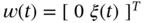 , and
, and  is zero mean white Gaussian noise with the variance
  . Plot the first and second states of the system as functions of time for
  ,
,  , and
, and  . Analyze the difference between functions.
 - A system is represented with the state‐space model in (1.11) and (1.12), where
 and
and  . Assume that noise vectors
  and
and  are correlated,

where
 ,
,  , and
, and  . Analyze intuitively how the correlation will affect the state estimate if we neglect it by setting
  in the algorithm.
 - The general structures of FIR and limited memory IIR estimators are shown in Fig. 1.1a and Fig. 1.1b, respectively. Explain logically why the initial
 and
and  serve as variables of the FIR estimator gain, while
  is an input of the limited memory IIR estimator.
 - In a satellite navigation system, the geometric distance
 between the receiver and the
  th satellite is measured as

where
 are 3D ground coordinates and
  are 3D coordinates of the
  th satellite. High navigation accuracy is guaranteed by the estimation of distance, velocity, and acceleration. Determine the dimensions of the navigation state vector.
 - The dynamics of a DC motor are described by the following equations,

where
 is the angle of rotation,
  is the armature current,
  is the electric resistance,
  is the electric inductance,
  is the motor viscous friction constant,
  is the moment of inertia of the rotor,
  is the driving voltage, and
  represents the motor torque and back electromotive force constants. The
  measurements are performed in the presence of noise
  . Introduce the state vector
  and represent the motor equations and measurement in continuous time state space.
 - A dynamic physical system is represented in continuous time state space with the state space equations
 and
and  , where matrices are of the form

Determine the dimensions of vectors
 and
and  and write the differential equation for this system.
 - Find the conditions under which the RH FIR estimator shown in Fig. 1.2c becomes a special case of the FIR estimator shown in Fig. 1.2a.
- The autonomous system consists of two subsystems [211],

where
 and matrices are specified as
Investigate numerically the impulse responses of these systems.
- Local clocks are characterized by three variables that represent their states: 1)
 is the time error, 2)
  is the fractional frequency offset, and 3)
  is the linear frequency drift rate. Variables are disturbed by independent noise sources. Write down the clock state model in discrete time.
 - An electronic oscillator is represented with the SDE

where
 is the generated voltage,
  is the angular bandwidth,
  is the oscillator angular frequency, and noise
  has the variance
  . Represent this equation in state space.
 - The block diagram of a stochastic LTV system, which is represented in continuous‐time state space, is shown in Fig. 1.4. Write the state space equations of this system.

Figure 1.4 Block diagram of a stochastic LTV system observed in continuous time state space.
- The system state
 is observed over a horizon
  in the presence of zero mean measurement noise
  as
as  , where

Show that the gain
 of an UFIR filter
  that satisfies the unbiasedness condition (1.31) is given by
Compare this gain to the canonic gain of the UFIR state estimator defined by (1.32) and analyze the differences.
- The time‐invariant gain
 of the median filter is given by (1.21) with
  . Approximate the absolute error
  with a differentiable function
  such that at the limit it is equal to
  . Minimize the sum
  by
by  using the derivative and obtain a closed form for
  in the limit.
Notes
- 1 Note that the infinity error norm has another meaning than the standard vector infinity norm.
- 2 Johannes Kepler (December 27, 1571 to November 15, 1630), German astronomer, mathematician, and astrologer.
- 3 Johann Carl Friedrich Gauss (April 30, 1777 to Feb 23, 1855), German mathematician and physicist.
- 4 Andrey Nikolaevich Kolmogorov (April 25, 1903 to October 20, 1987), Soviet mathematician.
- 5 Norbert Wiener (November 26, 1894 to March 18, 1964), American mathematician and philosopher.
- 6 Rudolf Emil Kálmán (May 19, 1930 to July 2, 2016), Hungarian‐American electrical engineer, mathematician, and inventor.
- 7 Thomas Bayes (1701 to April 7, 1761), English statistician, philosopher, and Presbyterian minister.
- 8 Ruslan Leont'evich Stratonovich (May 31, 1930 to January 13, 1997), Russian physicist, engineer, and probabilist.
- 9 Lotfi Aliasker Zadeh (February 4, 1921 to September 6, 2017), Iranian‐American mathematician, computer scientist, electrical engineer.