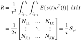
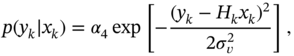
3
State Estimation
Gauss's batch least squares is routinely used today, and it often gives accuracy that is superior to the best available EKF.
Fred Daum, [40], p. 65
Although SDEs provide accessible mathematical models and have become standard models in many areas of science and engineering, features extraction from high‐order processes is usually much more complex than from first‐order processes such as the Langevin equation. The state-space representation avoids many inconveniences by replacing high‐order SDEs with first‐order vector SDEs. Estimation performed using the state‐space model solves simultaneously two problems: 1) filtering measurement noise and, in some cases, process noise and thus filter, and 2) solving state‐space equations with respect to the process state and thus state estimator. For well‐defined linear models, state estimation is usually organized using optimal, optimal unbiased, and unbiased estimators. However, any uncertainty in the model, interference, and/or errors in the noise description may require a norm‐bounded state estimator to obtain better results. Methods of linear state estimation can be extended to nonlinear problems to obtain acceptable estimates in the case of smooth nonlinearities. Otherwise, special nonlinear estimators can be more successful in accuracy. In this chapter, we lay the foundations of state estimation and introduce the reader to the most widely used methods applied to linear and nonlinear stochastic systems and processes.
3.1 Lineal Stochastic Process in State Space
To introduce the state space approach, we consider a simple case of a single‐input, single‐output ![]() th order LTV system represented by the SDE
th order LTV system represented by the SDE

where ![]() ,
, ![]() , and
, and ![]() are known time‐varying coefficients;
are known time‐varying coefficients; ![]() is the output;
is the output; ![]() is the input; and
is the input; and ![]() is WGN. To represent (3.1) in state space, let us assign
is WGN. To represent (3.1) in state space, let us assign ![]() , suppose that
, suppose that ![]() , and rewrite (3.1) as
, and rewrite (3.1) as

The ![]() th‐order derivative in (3.2) can be viewed as the
th‐order derivative in (3.2) can be viewed as the ![]() th system state and the state variables
th system state and the state variables ![]() assigned as
assigned as

to be further combined into compact matrix forms
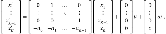
called state‐space equations, where time ![]() is omitted for simplicity. In a similar manner, a multiple input multiple output (MIMO) system can be represented in state space.
is omitted for simplicity. In a similar manner, a multiple input multiple output (MIMO) system can be represented in state space.
In applications, the system output ![]() is typically measured in the presence of additive noise
is typically measured in the presence of additive noise ![]() and observed as
and observed as ![]() . Accordingly, a continuous‐time MIMO system can be represented in state space using the state equation and observation equation, respectively, as
. Accordingly, a continuous‐time MIMO system can be represented in state space using the state equation and observation equation, respectively, as
where ![]() is the state vector,
is the state vector, ![]() ,
, ![]() is the observation vector,
is the observation vector, ![]() is the input (control) signal vector,
is the input (control) signal vector, ![]() is the process noise, and
is the process noise, and ![]() is the observation or measurement noise. Matrices
is the observation or measurement noise. Matrices ![]() ,
, ![]() ,
, ![]() .
. ![]() , and
, and ![]() are generally time‐varying. Note that the term
are generally time‐varying. Note that the term ![]() appears in (3.4) only if the order of
appears in (3.4) only if the order of ![]() is the same as of the system,
is the same as of the system, ![]() . Otherwise, this term must be omitted. Also, if a system has no input, then both terms consisting
. Otherwise, this term must be omitted. Also, if a system has no input, then both terms consisting ![]() in (3.3) and (3.4) must be omitted. In what follows, we will refer to the following definition of the state space linear SDE.
in (3.3) and (3.4) must be omitted. In what follows, we will refer to the following definition of the state space linear SDE.
Linear SDE in state‐space: The model in ((3.3)) and ((3.4)) is called linear if all its noise processes are Gaussian.
3.1.1 Continuous‐Time Model
Solutions to (3.3) and (3.4) can be found in state space in two different ways for LTI and LTV systems.
Time‐Invariant Case
When modeling LTI systems, all matrices are constant, and the solution to the state equation 3.3 can be found by multiplying both sides of (3.3) from the left‐hand side with an integration factor ![]() ,
,
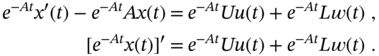
Further integration from ![]() to
to ![]() gives
gives

and the solution becomes

where the state transition matrix that projects the state from ![]() to
to ![]() is
is
and ![]() is called matrix exponential. Note that the stochastic integral in (3.6) can be computed either in the Itô sense or in the Stratonovich sense [193].
is called matrix exponential. Note that the stochastic integral in (3.6) can be computed either in the Itô sense or in the Stratonovich sense [193].
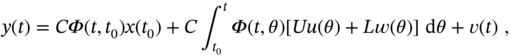
Substituting (3.6) into (3.4) transforms the observation equation to
where the matrix exponential ![]() has Maclaurin series
has Maclaurin series
in which ![]() is an identity matrix. The matrix exponential
is an identity matrix. The matrix exponential ![]() can also be transformed using the Cayley‐Hamilton theorem [167], which states that
can also be transformed using the Cayley‐Hamilton theorem [167], which states that ![]() can be represented with a finite series of length
can be represented with a finite series of length ![]() as
as
if a constant ![]() ,
, ![]() , is specified properly.
, is specified properly.
Time‐Varying Case
For equations 3.3 and (3.4) of the LTV system with time‐varying matrices, the proper integration factor cannot be found to obtain solutions like for (3.6) and (3.8) [167]. Instead, one can start with a homogenous ordinary differential equation (ODE) [28]
Matrix theory suggests that if ![]() is continuous for
is continuous for ![]() , then the solution to (3.13) for a known initial
, then the solution to (3.13) for a known initial ![]() can be written as
can be written as
where the fundamental matrix ![]() that satisfies the differential equation
that satisfies the differential equation
is nonsingular for all ![]() and is not unique.
and is not unique.
To determine ![]() , we can consider
, we can consider ![]() initial state vectors
initial state vectors ![]() , obtain from (3.13)
, obtain from (3.13) ![]() solutions
solutions ![]() , and specify the fundamental matrix as
, and specify the fundamental matrix as ![]() . Since each particular solution satisfies (3.13), it follows that matrix
. Since each particular solution satisfies (3.13), it follows that matrix ![]() defined in this way satisfies (3.14).
defined in this way satisfies (3.14).
Provided ![]() , the solution to (3.13) can be written as
, the solution to (3.13) can be written as ![]() , where
, where ![]() satisfies (3.15), and
satisfies (3.15), and ![]() is some unknown function of the same class. Referring to (3.15), equation 3.3 can then be transformed to
is some unknown function of the same class. Referring to (3.15), equation 3.3 can then be transformed to
and, from (3.16), we have
which, by known ![]() , specifies function
, specifies function ![]() as
as
The solution to (3.3), by ![]() and (3.17), finally becomes
and (3.17), finally becomes
where the state transition matrix is given by
Referring to (3.18), the observation equation can finally be rewritten as

It should be noted that the solutions (3.6) and (3.19) are formally equivalent. The main difference lies in the definitions of the state transition matrix: (3.7) for LTI systems and (3.19) for LTV systems.
3.1.2 Discrete‐Time Model
The necessity of representing continuous‐time state‐space models in discrete time arises when numerical analysis is required or solutions are supposed to be obtained using digital blocks. In such cases, a solution to an SDE is considered at two discrete points ![]() and
and ![]() with a time step
with a time step ![]() , where
, where ![]() is a discrete time index. It is also supposed that a digital
is a discrete time index. It is also supposed that a digital ![]() represents accurately a discrete‐time
represents accurately a discrete‐time ![]() . Further, the FE or BE methods are used [26].
. Further, the FE or BE methods are used [26].
The FE method, also called the standard Euler method or Euler‐Maruyama method, relates the numerically computed stochastic integrals to ![]() and is associated with Itô calculus. The relevant discrete‐time state‐space model
and is associated with Itô calculus. The relevant discrete‐time state‐space model ![]() , sometimes called a prediction model, is basic in control. A contradiction here is with the noise term
, sometimes called a prediction model, is basic in control. A contradiction here is with the noise term ![]() that exists even though the initial state
that exists even though the initial state ![]() is supposed to be known and thus already affected by
is supposed to be known and thus already affected by ![]() .
.
The BE method, also known as an implicit method, relates all integrals to the current time ![]() that yields
that yields ![]() . This state equation is sometimes called a real‐time model and is free of the contradiction inherent to the FE‐based state equation.
. This state equation is sometimes called a real‐time model and is free of the contradiction inherent to the FE‐based state equation.
The FE and BE methods are uniquely used to convert continuous‐time differential equations to discrete time, and in the sequel we will use both of them. It is also worth noting that predictive state estimators fit better with the FE method and filters with the BE method.
Time‐Invariant Case
Consider the solution (3.6) and the observation (3.4), substitute ![]() with
with ![]() ,
, ![]() with
with ![]() , and write
, and write

Because input ![]() is supposed to be known, assume that it is also piecewise constant on each time step and put
is supposed to be known, assume that it is also piecewise constant on each time step and put ![]() outside the first integral. Next, substitute
outside the first integral. Next, substitute ![]() ,
, ![]() , and
, and ![]() , and write
, and write
where ![]() ,
, ![]() , and
, and


The discrete process noise ![]() given by (3.24) has zero mean,
given by (3.24) has zero mean, ![]() , and the covariance
, and the covariance ![]() specified using the continuous WGN covariance (2.91) by
specified using the continuous WGN covariance (2.91) by

Observe that ![]() is a matrix of the same class as
is a matrix of the same class as ![]() , which is a function of
, which is a function of ![]() ,
, ![]() . If
. If ![]() is small enough, then this term can be set to zero. If also
is small enough, then this term can be set to zero. If also ![]() in (3.3), then
in (3.3), then ![]() establishes a rule of thumb relationship between the discrete and continuous process noise covariances.
establishes a rule of thumb relationship between the discrete and continuous process noise covariances.
The zero mean discrete observation noise ![]() (2.93) has the covariance
(2.93) has the covariance ![]() defined as
defined as
where ![]() ,
, ![]() , is a component of the PSD matrix
, is a component of the PSD matrix ![]() .
.
Time‐Varying Case
For LTV systems, solutions in state space are given by (3.18) and (3.20). Substituting ![]() with
with ![]() and
and ![]() with
with ![]() yields
yields
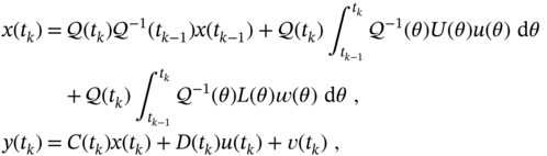
where the fundamental matrix ![]() must be assigned individually for each model. Reasoning along similar lines as for LTI systems, these equations can be represented in discrete‐time as
must be assigned individually for each model. Reasoning along similar lines as for LTI systems, these equations can be represented in discrete‐time as
where ![]() and the time‐varying matrices are given by
and the time‐varying matrices are given by

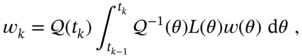
and noise ![]() has zero mean,
has zero mean, ![]() , and generally a time‐varying covariance
, and generally a time‐varying covariance ![]() . Noise
. Noise ![]() also has zero mean,
also has zero mean, ![]() , and generally a time‐varying covariance
, and generally a time‐varying covariance ![]() .
.
3.2 Methods of Linear State Estimation
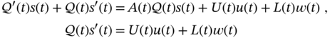
Provided adequate modeling of a real linear physical process in discrete‐time state space, state estimation can be carried out using methods of optimal linear filtering based on the following state‐space equations,
where ![]() is the state vector,
is the state vector, ![]() is the input (or control) signal vector,
is the input (or control) signal vector, ![]() is the observation (or measurement) vector,
is the observation (or measurement) vector, ![]() is the system (process) matrix,
is the system (process) matrix, ![]() is the observation matrix,
is the observation matrix, ![]() is the control (or input) matrix,
is the control (or input) matrix, ![]() is the disturbance matrix, and
is the disturbance matrix, and ![]() is the system (or process) noise matrix. The term with
is the system (or process) noise matrix. The term with ![]() is usually omitted in (3.33), assuming that the order of
is usually omitted in (3.33), assuming that the order of ![]() is less than the order of
is less than the order of ![]() . At the other extreme, when the input disturbance appears to be severe, the noise components are often omitted in (3.32) and (3.33).
. At the other extreme, when the input disturbance appears to be severe, the noise components are often omitted in (3.32) and (3.33).
In many cases, system or process noise is assumed to be zero mean and white Gaussian ![]() with known covariance
with known covariance ![]() . Measurement or observation noise
. Measurement or observation noise ![]() is also often modeled as zero mean and white Gaussian with covariance
is also often modeled as zero mean and white Gaussian with covariance ![]() . Moreover, many problems suggest that
. Moreover, many problems suggest that ![]() and
and ![]() can be viewed as physically uncorrelated and independent processes. However, there are other cases when
can be viewed as physically uncorrelated and independent processes. However, there are other cases when ![]() and
and ![]() are correlated with each other and exhibit different kinds of coloredness.
are correlated with each other and exhibit different kinds of coloredness.
Filters of two classes can be designed to provide state estimation based on (3.32) and (3.33). Estimators of the first class ignore the process dynamics described by the state equation 3.32. Instead, they require multiple measurements of the quantity in question to approach the true value through statistical averaging. Such estimators have batch forms, but recursive forms may also be available. An example is the LS estimator. Estimators of the second class require both state‐space equations, so they are more flexible and universal. The recursive KF algorithm belongs to this class of estimators, but its batch form is highly inefficient in view of growing memory due to IIR. The batch FIR filter and LMF, both operating on finite horizons, are more efficient in this sense, but they cause computational problems when the batch is very large.
Regardless of the estimator structure, the notation ![]() means an estimate of the state
means an estimate of the state ![]() at time index
at time index ![]() , given observations of
, given observations of ![]() up to and including at time index
up to and including at time index ![]() . The state
. The state ![]() to be estimated at the time index
to be estimated at the time index ![]() is represented by the following standard variables:
is represented by the following standard variables:
![]()
![]() is the a priori (or prior) state estimate at
is the a priori (or prior) state estimate at ![]() given observations up to and including at time index
given observations up to and including at time index ![]() ;
;
![]()
![]() is the a posteriori (or posterior) state estimate at
is the a posteriori (or posterior) state estimate at ![]() given observations up to and including at
given observations up to and including at ![]() ;
;
![]() The a priori estimation error is defined by
The a priori estimation error is defined by
![]() The a posteriori estimation error is defined by
The a posteriori estimation error is defined by
![]() The a priori error covariance is defined by
The a priori error covariance is defined by
![]() The a posteriori error covariance is defined by
The a posteriori error covariance is defined by
In what follows, we will refer to these definitions in the derivation and study of various types of state estimators.
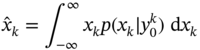
3.2.1 Bayesian Estimator
Suppose there is some discrete stochastic process ![]() ,
, ![]() measured as
measured as ![]() and assigned a set of measurements
and assigned a set of measurements ![]() . We may also assume that the a posteriori density
. We may also assume that the a posteriori density ![]() is known at the past time index
is known at the past time index ![]() . Of course, our interest is to obtain the a posteriori density
. Of course, our interest is to obtain the a posteriori density ![]() at
at ![]() . Provided
. Provided ![]() , the estimate
, the estimate ![]() can be found as the first‐order initial moment (2.10) and the estimation error as the second‐order central moment (2.14). To this end, we use Bayes' rule (2.43) and obtain
can be found as the first‐order initial moment (2.10) and the estimation error as the second‐order central moment (2.14). To this end, we use Bayes' rule (2.43) and obtain ![]() as follows.
as follows.
Consider the join density ![]() and represent it as
and represent it as

Note that ![]() is independent of past measurements and write
is independent of past measurements and write ![]() . Also, the desirable a posteriori pdf can be written as
. Also, the desirable a posteriori pdf can be written as ![]() . Then use Bayesian inference (2.47) and obtain
. Then use Bayesian inference (2.47) and obtain

where ![]() is a normalizing constant, the conditional density
is a normalizing constant, the conditional density ![]() represents the prior distribution of
represents the prior distribution of ![]() , and
, and ![]() is the likelihood function of
is the likelihood function of ![]() given the outcome
given the outcome ![]() . Note that the conditional pdf
. Note that the conditional pdf ![]() can be expressed via known
can be expressed via known ![]() using the rule (2.53) as
using the rule (2.53) as

Provided ![]() , the Bayesian estimate is obtained by (2.10) as
, the Bayesian estimate is obtained by (2.10) as
and the estimation error is obtained by (2.14) as

From the previous, it follows that the Bayesian estimate (3.41) is universal regardless of system models and noise distributions.
Bayesian estimator: Bayesian estimation can be universally applied to linear and nonlinear models with Gaussian and non‐Gaussian noise.
It is worth noting that for linear models the Bayesian approach leads to the optimal KF algorithm, which will be shown next.
Linear Model
Let us look at an important special case and show how the Bayesian approach can be applied to a linear Gaussian model (3.32) and (3.33) with ![]() . For clarity, consider a first‐order stochastic process. The goal is to obtain the a posteriori density
. For clarity, consider a first‐order stochastic process. The goal is to obtain the a posteriori density ![]() in terms of the known a posteriori density
in terms of the known a posteriori density ![]() and arrive at a computational algorithm.
and arrive at a computational algorithm.
To obtain the desired ![]() using (3.39), we need to specify
using (3.39), we need to specify ![]() using (3.40) and define the likelihood function
using (3.40) and define the likelihood function ![]() . Noting that all distributions are Gaussian, we can represent
. Noting that all distributions are Gaussian, we can represent ![]() as
as

where ![]() is the known a posteriori estimate of
is the known a posteriori estimate of ![]() and
and ![]() is the variance of the estimation error. Hereinafter, we will use
is the variance of the estimation error. Hereinafter, we will use ![]() as the normalizing coefficient.
as the normalizing coefficient.
Referring to (3.32), the conditional density ![]() can be written as
can be written as

where ![]() is the variance of the process noise
is the variance of the process noise ![]() .
.
Now, the a priori density ![]() can be transformed using (3.40) as
can be transformed using (3.40) as

By substituting (3.43) and (3.44) and equating to unity the integral of the normally distributed ![]() , (3.45) can be transformed to
, (3.45) can be transformed to

Likewise, the likelihood function ![]() can be written using (3.33) as
can be written using (3.33) as
where ![]() is the variance of the observation noise
is the variance of the observation noise ![]() . Then the required density
. Then the required density ![]() can be represented by (3.39) using (3.46) and (3.47) as
can be represented by (3.39) using (3.46) and (3.47) as

which holds if the following obvious relationship is satisfied
By equating to zero the free term and terms with ![]() and
and ![]() , we arrive at several conditions
, we arrive at several conditions


which establish a recursive computational algorithm to compute the estimate ![]() (3.53) and the estimation error
(3.53) and the estimation error ![]() (3.50) starting with the initial
(3.50) starting with the initial ![]() and
and ![]() for known
for known ![]() and
and ![]() . This is a one‐state KF algorithm. What comes from its derivation is that the estimate (3.53) is obtained without using (3.41) and (3.42). Therefore, it is not a Bayesian estimator. Later, we will derive the
. This is a one‐state KF algorithm. What comes from its derivation is that the estimate (3.53) is obtained without using (3.41) and (3.42). Therefore, it is not a Bayesian estimator. Later, we will derive the ![]() ‐state KF algorithm and discuss it in detail.
‐state KF algorithm and discuss it in detail.
3.2.2 Maximum Likelihood Estimator
From (3.39) it follows that the a posteriori density ![]() is given in terms of the a priori density
is given in terms of the a priori density ![]() and the likelihood function
and the likelihood function ![]() . It is also worth knowing that the likelihood function plays a special role in the estimation theory, and its use leads to the ML state estimator. For the first‐order Gaussian stochastic process, the likelihood function is given by the expression (3.47). This function is maximized by minimizing the exponent power, and we see that the only solution following from
. It is also worth knowing that the likelihood function plays a special role in the estimation theory, and its use leads to the ML state estimator. For the first‐order Gaussian stochastic process, the likelihood function is given by the expression (3.47). This function is maximized by minimizing the exponent power, and we see that the only solution following from ![]() is inefficient due to noise.
is inefficient due to noise.
An efficient ML estimate can be obtained if we combine ![]() measurement samples of the fully observed vector
measurement samples of the fully observed vector ![]() into an extended observation vector
into an extended observation vector ![]() with a measurement noise
with a measurement noise ![]() and write the observation equation as
and write the observation equation as
where ![]() is the extended observation matrix. A relevant example can be found in sensor networks, where the desired quantity is simultaneously measured by
is the extended observation matrix. A relevant example can be found in sensor networks, where the desired quantity is simultaneously measured by ![]() sensors. Using (3.54), the ML estimate of
sensors. Using (3.54), the ML estimate of ![]() can be found by maximizing the likelihood function
can be found by maximizing the likelihood function ![]() as
as
For Gaussian processes, the likelihood function becomes

where ![]() is the extended covariance matrix of the measurement noise
is the extended covariance matrix of the measurement noise ![]() . Since maximizing (3.56) with (3.55) means minimizing the power of the exponent, the ML estimate can equivalently be obtained from
. Since maximizing (3.56) with (3.55) means minimizing the power of the exponent, the ML estimate can equivalently be obtained from
By equating the derivative with respect to ![]() to zero,
to zero,
using the identities (A.4) and (A.5), and assuming that ![]() is nonsingular, the ML estimate can be found as
is nonsingular, the ML estimate can be found as
which demonstrates several important properties when the number ![]() of measurement samples grows without bound [125]:
of measurement samples grows without bound [125]:
- It converges to the true value of
 .
. - It is asymptotically optimal unbiased, normally distributed, and efficient.
Maximum likelihood estimate [125]: There is no other unbiased estimate whose covariance is smaller than the finite covariance of the ML estimate as a number of measurement samples grows without bounds.
It follows from the previous that as ![]() increases, the ML estimate (3.58) converges to the Bayesian estimate (3.41). Thus, the ML estimate has the property of unbiased optimality when
increases, the ML estimate (3.58) converges to the Bayesian estimate (3.41). Thus, the ML estimate has the property of unbiased optimality when ![]() grows unboundedly, and is inefficient when
grows unboundedly, and is inefficient when ![]() is small.
is small.
3.2.3 Least Squares Estimator
Another approach to estimate ![]() from (3.54) is known as Gauss' least squares (LS) [54,185] or LS estimator,1 which is widely used in practice. In the LS method, the estimate
from (3.54) is known as Gauss' least squares (LS) [54,185] or LS estimator,1 which is widely used in practice. In the LS method, the estimate ![]() is chosen such that the sum of the squares of the residuals
is chosen such that the sum of the squares of the residuals ![]() minimizes the cost function
minimizes the cost function ![]() over all
over all ![]() to obtain
to obtain
Reasoning similarly to (3.57), the estimate can be found to be
To improve (3.60), we can consider the weighted cost function ![]() , in which
, in which ![]() is a symmetric positive definite weight matrix. Minimizing of this cost yields the weighted LS (WLS) estimate
is a symmetric positive definite weight matrix. Minimizing of this cost yields the weighted LS (WLS) estimate
and we infer that the ML estimate (3.58) is a special case of WLS estimate (3.61), in which ![]() is chosen to be the measurement noise covariance
is chosen to be the measurement noise covariance ![]() .
.
3.2.4 Unbiased Estimator
If someone wants an unbiased estimator, whose average estimate is equal to the constant ![]() , then the only performance criterion will be
, then the only performance criterion will be
To obtain an unbiased estimate, one can think of an estimate ![]() as the product of some gain
as the product of some gain ![]() and the measurement vector
and the measurement vector ![]() given by (3.54),
given by (3.54),
Since ![]() has zero mean, the unbiasedness condition (3.62) gives the unbiasedness constraint
has zero mean, the unbiasedness condition (3.62) gives the unbiasedness constraint
By multiplying the constraint by the identity ![]() from the right‐hand side and discarding the nonzero
from the right‐hand side and discarding the nonzero ![]() on both sides, we obtain
on both sides, we obtain ![]() and arrive at the unbiased estimate
and arrive at the unbiased estimate
which is identical to the LS estimate (3.60). Since the product ![]() is associated with discrete convolution, the unbiased estimator (3.63) can be thought of as an unbiased FIR filter.
is associated with discrete convolution, the unbiased estimator (3.63) can be thought of as an unbiased FIR filter.
Recursive Unbiased (LS) Estimator
We have already mentioned that batch estimators (3.63) and (3.60) can be computationally inefficient and cause a delay when the number of data points ![]() is large. To compute the batch estimate recursively, one can start with
is large. To compute the batch estimate recursively, one can start with ![]() ,
, ![]() , associated with matrix
, associated with matrix ![]() , and rewrite (3.63) as
, and rewrite (3.63) as
where ![]() . Further, matrix
. Further, matrix ![]() can be represented using the forward and backward recursions as [179]
can be represented using the forward and backward recursions as [179]
and ![]() rewritten similarly as
rewritten similarly as
Combining this recursive form with (3.64), we obtain
Next, substituting ![]() taken from (3.64), combining with (3.66), and providing some transformations gives the recursive form
taken from (3.64), combining with (3.66), and providing some transformations gives the recursive form
in which ![]() can be computed recursively by (3.65). To run the recursions, the variable
can be computed recursively by (3.65). To run the recursions, the variable ![]() must range as
must range as ![]() for the inverse in (3.64) to exist and the initial values calculated at
for the inverse in (3.64) to exist and the initial values calculated at ![]() using the original batch forms.
using the original batch forms.
3.2.5 Kalman Filtering Algorithm
We now look again at the recursive algorithm in (3.50)–(3.53) associated with one‐state linear models. The approach can easily be extended to the ![]() ‐state linear model
‐state linear model
where the noise vectors ![]() and
and ![]() are uncorrelated. The corresponding algorithm was derived by Kalman in his seminal paper [84] and is now commonly known as the Kalman filter.2
are uncorrelated. The corresponding algorithm was derived by Kalman in his seminal paper [84] and is now commonly known as the Kalman filter.2
The KF algorithm operates in two phases: 1) in the prediction phase, the a priori estimate and error covariance are predicted at ![]() using measurements at
using measurements at ![]() , and 2) in the update phase, the a priori values are updated at
, and 2) in the update phase, the a priori values are updated at ![]() to the a posteriori estimate and error covariance using measurements at
to the a posteriori estimate and error covariance using measurements at ![]() . This strategy assumes two available algorithmic options: the a posteriori KF algorithm and the a priori KF algorithm. It is worth noting that the original KF algorithm is a posteriori.
. This strategy assumes two available algorithmic options: the a posteriori KF algorithm and the a priori KF algorithm. It is worth noting that the original KF algorithm is a posteriori.
The a posteriori Kalman Filter
Consider a ![]() ‐state space model as in (3.68) and (3.69). The Bayesian approach can be applied similarly to the one‐state case, as was done by Kalman in [84], although there are several other ways to arrive at the KF algorithm. Let us show the simplest one.
‐state space model as in (3.68) and (3.69). The Bayesian approach can be applied similarly to the one‐state case, as was done by Kalman in [84], although there are several other ways to arrive at the KF algorithm. Let us show the simplest one.
The first thing to note is that the most reasonable prior estimate can be taken from (3.68) for the known estimate ![]() and input
and input ![]() if we ignore the zero mean noise
if we ignore the zero mean noise ![]() . This gives
. This gives
which is also the prior estimate (3.52).
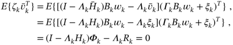
To update ![]() , we need to involve the observation (3.69). This can be done if we take into account the measurement residual
, we need to involve the observation (3.69). This can be done if we take into account the measurement residual
which is the difference between data ![]() and the predicted data
and the predicted data ![]() . The measurement residual covariance
. The measurement residual covariance ![]() can then be written as
can then be written as

Since ![]() is generally biased, because
is generally biased, because ![]() is generally biased, the prior estimate can be updated as
is generally biased, the prior estimate can be updated as
where the matrix ![]() is introduced to correct the bias in
is introduced to correct the bias in ![]() . Therefore,
. Therefore, ![]() plays the role of the bias correction gain.
plays the role of the bias correction gain.
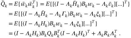
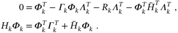
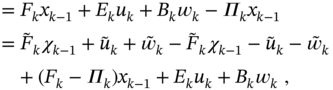
As can be seen, the relations (3.70) and (3.73), which are reasonably extracted from the state‐space model, are exactly the relations (3.52) and (3.53). Now notice that the estimate (3.73) will be optimal if we will find ![]() such that the MSE is minimized. To do this, let us refer to (3.68) and (3.69) and define errors (3.34)–(3.37) involving (3.70)–(3.73).
such that the MSE is minimized. To do this, let us refer to (3.68) and (3.69) and define errors (3.34)–(3.37) involving (3.70)–(3.73).
The prior estimation error ![]() (3.34) can be transformed as
(3.34) can be transformed as

and, for mutually uncorrelated ![]() and
and ![]() , the prior error covariance (3.36) can be transformed to
, the prior error covariance (3.36) can be transformed to
Next, the estimation error ![]() (3.35) can be represented by
(3.35) can be represented by
and, for mutually uncorrelated ![]() ,
, ![]() , and
, and ![]() , the a posteriori error covariance (3.37) can be transformed to
, the a posteriori error covariance (3.37) can be transformed to

What is left behind is to find the optimal bias correction gain ![]() that minimizes MSE. This can be done by minimizing the trace of
that minimizes MSE. This can be done by minimizing the trace of ![]() , which is a convex function with a minimum corresponding to the optimal
, which is a convex function with a minimum corresponding to the optimal ![]() . Using the matrix identities (A.3) and (A.6), the minimization of
. Using the matrix identities (A.3) and (A.6), the minimization of ![]() by
by ![]() can be carried out if we rewrite the equation
can be carried out if we rewrite the equation ![]() as
as
This gives the optimal bias correction gain
The gain ![]() (3.78) is known as the Kalman gain, and its substitution on the left‐hand side of the last term in (3.77) transforms the error covariance
(3.78) is known as the Kalman gain, and its substitution on the left‐hand side of the last term in (3.77) transforms the error covariance ![]() into
into
Another useful form of ![]() appears when we first refer to (3.78) and (3.72) and transform (3.77) as
appears when we first refer to (3.78) and (3.72) and transform (3.77) as

Next, inverting the both sides of ![]() and applying (A.7) gives [185]
and applying (A.7) gives [185]

and another form of ![]() appears as
appears as
Using (3.80), the Kalman gain (3.78) can also be modified as [185]

The previous derived standard KF algorithm gives an estimate at ![]() utilizing data from zero to
utilizing data from zero to ![]() . Therefore, it is also known as the a posteriori KF algorithm, the pseudocode of which is listed as Algorithm 1. The algorithm requires initial values
. Therefore, it is also known as the a posteriori KF algorithm, the pseudocode of which is listed as Algorithm 1. The algorithm requires initial values ![]() and
and ![]() , as well as noise covariances
, as well as noise covariances ![]() and
and ![]() to update the estimates starting at
to update the estimates starting at ![]() . Its operation is quite transparent, and recursions are easy to program, are fast to compute, and require little memory, making the KF algorithm suitable for many applications.
. Its operation is quite transparent, and recursions are easy to program, are fast to compute, and require little memory, making the KF algorithm suitable for many applications.
The a priori Kalman Filter
Unlike the a posteriori KF, the a priori KF gives an estimate at ![]() using data
using data ![]() from
from ![]() . The corresponding algorithm emerges from Algorithm 1 if we first substitute (3.79) in (3.74) and go to the discrete difference Riccati equation (DDRE)
. The corresponding algorithm emerges from Algorithm 1 if we first substitute (3.79) in (3.74) and go to the discrete difference Riccati equation (DDRE)
which gives recursion for the covariance of the prior estimation error. Then the a priori estimate ![]() can be obtained by the transformations
can be obtained by the transformations
and the a priori KF formalized with the pseudocode specified in Algorithm 2. As can be seen, this algorithm does not require data ![]() to produce an estimate at
to produce an estimate at ![]() . However, it requires future values
. However, it requires future values ![]() and
and ![]() and is thus most suitable for LTI systems without input.
and is thus most suitable for LTI systems without input.
Optimality and Unbiasedness of the Kalman Filter
From the derivation of the Kalman gain (3.78) it follows that, by minimizing the MSE, the KF becomes optimal [36,220]. In Chapter, the optimality of KF will be supported by the batch OFIR filter, whose recursions are exactly the KF recursions. On the other hand, the KF originates from the Bayesian approach. Therefore, many authors also call it optimal unbiased, and the corresponding proof given in [54] has been mentioned in many works [9,58,185]. However, in Chapter it will be shown that the batch OUFIR filter has other recursions, which contradicts the proof given in [54].
To ensure that the KF is optimal, let us look at the explanation given in [54]. So let us consider the model (3.68) with ![]() and define an estimate
and define an estimate ![]() as [54]
as [54]
where ![]() and the gain
and the gain ![]() still needs to be determined. Next, let us examine the a priori error
still needs to be determined. Next, let us examine the a priori error ![]() and the a posteriori error
and the a posteriori error

Estimate (3.82) was stated in [54], p. 107, to be unbiased if ![]() and
and ![]() . By satisfying these conditions using the previous relations, we obtain
. By satisfying these conditions using the previous relations, we obtain ![]() and the KF estimate becomes (3.73). This fact was used in [54] as proof that the KF is optimal unbiased.
and the KF estimate becomes (3.73). This fact was used in [54] as proof that the KF is optimal unbiased.
Now, notice that the prior error ![]() is always biased in dynamic systems, so
is always biased in dynamic systems, so ![]() . Otherwise, there would be no need to adjust the bias by
. Otherwise, there would be no need to adjust the bias by ![]() . Then we redefine the prior estimate as
. Then we redefine the prior estimate as
and average the estimation error as

The filter will be unbiased if ![]() is equal to zero that gives
is equal to zero that gives
Substituting (3.84) into (3.82) gives the same estimate (3.73) with, however, different ![]() defined by (3.83). The latter means that KF will be 1) optimal, if
defined by (3.83). The latter means that KF will be 1) optimal, if ![]() is optimally biased, and 2) optimal unbiased, if
is optimally biased, and 2) optimal unbiased, if ![]() has no bias. Now note that the Kalman gain
has no bias. Now note that the Kalman gain ![]() makes an estimate optimal, and therefore there is always a small bias to be found in
makes an estimate optimal, and therefore there is always a small bias to be found in ![]() , which contradicts the property of unbiased optimality and the claim that KF is unbiased.
, which contradicts the property of unbiased optimality and the claim that KF is unbiased.
Intrinsic Errors of Kalman Filtering
Looking at Algorithm 1 and assuming that the model matches the process, we notice that the required ![]() ,
, ![]() ,
, ![]() , and
, and ![]() must be exactly known in order for KF to be optimal. However, due to the practical impossibility of doing this at every
must be exactly known in order for KF to be optimal. However, due to the practical impossibility of doing this at every ![]() and prior to running the filter, these values are commonly estimated approximately, and the question arises about the practical optimality of KF. Accordingly, we can distinguish two intrinsic errors caused by incorrectly specified initial conditions and poorly known covariance matrices.
and prior to running the filter, these values are commonly estimated approximately, and the question arises about the practical optimality of KF. Accordingly, we can distinguish two intrinsic errors caused by incorrectly specified initial conditions and poorly known covariance matrices.
Figure 3.1 shows what happens to the KF estimate when ![]() and
and ![]() are set incorrectly. With correct initial values, the KF estimate ranges close to the actual behavior over all
are set incorrectly. With correct initial values, the KF estimate ranges close to the actual behavior over all ![]() . Otherwise, incorrectly set initial values can cause large initial errors and long transients. Although the KF estimate approaches an actual state asymptotically, it can take a long time. Such errors also occur when the process undergoes temporary changes associated, for example, with jumps in velocity, phase, and frequency. The estimator inability to track temporary uncertain behaviors causes transients that can last for a long time, especially in harmonic models [179].
. Otherwise, incorrectly set initial values can cause large initial errors and long transients. Although the KF estimate approaches an actual state asymptotically, it can take a long time. Such errors also occur when the process undergoes temporary changes associated, for example, with jumps in velocity, phase, and frequency. The estimator inability to track temporary uncertain behaviors causes transients that can last for a long time, especially in harmonic models [179].
Now, suppose the error covariances are not known exactly and introduce the worst‐case scaling factor ![]() as
as ![]() or
or ![]() . Figure 3.2 shows the typical root MSEs (RMSEs) produced by KF as functions of
. Figure 3.2 shows the typical root MSEs (RMSEs) produced by KF as functions of ![]() , and we notice that
, and we notice that ![]() makes the estimate noisy and
makes the estimate noisy and ![]() makes it biased with respect to the optimal case of
makes it biased with respect to the optimal case of ![]() . Although the most favorable case of
. Although the most favorable case of ![]() and
and ![]() assumes that the effects will be mutually exclusive, in practice this rarely happens due to the different nature of the process and measurement noise. We add that the intrinsic errors considered earlier appear at the KF output regardless of the model and differ only in values.
assumes that the effects will be mutually exclusive, in practice this rarely happens due to the different nature of the process and measurement noise. We add that the intrinsic errors considered earlier appear at the KF output regardless of the model and differ only in values.

Figure 3.1 Typical errors in the KF caused by incorrectly specified initial conditions. Transients can last for a long time, especially in a harmonic state‐space model.

Figure 3.2 Effect of errors in noise covariances,  and
and  , on the RMSEs produced by KF in the worst case:
  corresponds to the optimal estimate,
  makes the estimate more noisy, and
  makes it more biased.
3.2.6 Backward Kalman Filter
Some applications require estimating the past state of a process or retrieving information about the initial state and error covariance. For example, multi‐pass filtering (forward‐backward‐forward‐...) [231] updates the initial values using a backward filter, which improves accuracy.
The backward a posteriori KF can be obtained similarly to the standard KF if we represent the state equation 3.68 backward in time as
and then, reasoning along similar lines as for the a posteriori KF, define the a priori state estimate at ![]() ,
,
the measurement residual ![]() , the measurement residual covariance
, the measurement residual covariance
the backward estimate
the a priori error covariance
and the a posteriori error covariance
Further minimizing ![]() by
by ![]() gives the optimal gain
gives the optimal gain
and the modified error covariance
Finally, the pseudocode of the backward a posteriori KF, which updates the estimates from ![]() to 0, becomes as listed in Algorithm 3. The algorithm requires initial values
to 0, becomes as listed in Algorithm 3. The algorithm requires initial values ![]() and
and ![]() at
at ![]() and updates the estimates back in time from
and updates the estimates back in time from ![]() to zero to obtain estimates of the initial state
to zero to obtain estimates of the initial state ![]() and error covariance
and error covariance ![]() .
.
3.2.7 Alternative Forms of the Kalman Filter
Although the KF Algorithm 1 is the most widely used, other available forms of KF may be more efficient in some applications. Collections of such algorithms can be found in [9,58,185] and some other works. To illustrate the flexibility and versatility of KF in various forms, next we present two versions known as the information filter and alternate KF form. Noticing that these modifications were shown in [185] for the FE‐based model, we develop them here for the BE‐based model. Some other versions of the KF can be found in the section “Problems”.
Information Filter
When minimal information loss is required instead of minimal MSE, the information matrix ![]() , which is the inverse of the covariance matrix
, which is the inverse of the covariance matrix ![]() , can be used. Since
, can be used. Since ![]() is symmetric and positive definite, it follows that the inverse of
is symmetric and positive definite, it follows that the inverse of ![]() is unique and KF can be modified accordingly.
is unique and KF can be modified accordingly.
By introducing ![]() and
and ![]() , the error covariance (3.80) can be transformed to
, the error covariance (3.80) can be transformed to
where, by (3.75) and ![]() , matrix
, matrix ![]() becomes
becomes
Using the Woodbury identity (A.7), one can further rewrite (3.86) as
and arrive at the information KF [185]. Given ![]() ,
, ![]() ,
, ![]() ,
, ![]() , and
, and ![]() , the algorithm predicts and updates the estimates as
, the algorithm predicts and updates the estimates as
It is worth noting that the information KF is mathematically equivalent to the standard KF for linear models. However, its computational load is greater because more inversions are required in the covariance propagation.
Alternate Form of the KF
Another form of KF, called alternate KF form, has been proposed in [185] to felicitate obtaining optimal smoothing. The advantage is that this form is compatible with the game theory‐based ![]() filter [185]. The modification is provided by inverting the residual covariance (3.77) through the information matrix using (A.7). KF recursions modified in this way for a BE‐based model lead to the algorithm
filter [185]. The modification is provided by inverting the residual covariance (3.77) through the information matrix using (A.7). KF recursions modified in this way for a BE‐based model lead to the algorithm

It follows from [185] that matrix ![]() is equal to
is equal to ![]() . Therefore, this algorithm can be written in a more compact form. Given
. Therefore, this algorithm can be written in a more compact form. Given ![]() ,
, ![]() ,
, ![]() ,
, ![]() , and
, and ![]() , the initial prior error covariance is computed by
, the initial prior error covariance is computed by ![]() and the update equations for
and the update equations for ![]() become
become
The proof of the equivalence of matrices (3.92) and (3.77) is postponed to the section “Problems”.
3.2.8 General Kalman Filter
Looking into the KF derivation procedure, it can be concluded that the assumptions regarding the whiteness and uncorrelatedness of Gaussian noise are too strict and that the algorithm is thus “ideal,” since white noise does not exist in real life. More realistically, one can think of system noise and measurement noise as color processes and approximate them by a Gauss‐Markov process driven by white noise.
To make sure that such modifications are in demand in real life, consider a few examples. When noise passes through bandlimited and narrowband channels, it inevitably becomes colored and correlated. Any person traveling along a certain trajectory follows a control signal generated by the brain. Since this signal cannot be accurately modeled, deviations from its mean appear as system colored noise. A visual camera catches and tracks objects asymptotically, which makes the measurement noise colored.
In Fig. 3.3a, we give an example of the colored measurement noise (CMN) noise, and its simulation as the Gauss‐Markov process is illustrated in Fig. 3.3b. An example (Fig. 3.3a) shows the signal strength colored noise discovered in the GPS receiver [210]. The noise here was extracted by removing the antenna gain attenuation from the signal strength measurements and then normalizing to zero relative to the mean. The simulated colored noise shown in Fig. 3.3b comes from the Gauss‐Markov sequence ![]() with white Gaussian driving noise
with white Gaussian driving noise ![]() . Even a quick glance at the drawing (Fig. 3.3) allows us to think that both processes most likely belong to the same class and, therefore, colored noise can be of Markov origin.
. Even a quick glance at the drawing (Fig. 3.3) allows us to think that both processes most likely belong to the same class and, therefore, colored noise can be of Markov origin.
![Schematic illustration of examples of CMN in electronic channels: (a) signal strength CMN in a GPS receiver [210] and (c) Gauss-Markov noise simulated by vn=0.9vn-1+ξn with ξn∼(0,16).](https://imgdetail.ebookreading.net/2023/10/9781119863076/9781119863076__9781119863076__files__images__c03f003.png)
Figure 3.3 Examples of CMN in electronic channels: (a) signal strength CMN in a GPS receiver Based on [210] and (b) Gauss‐Markov noise simulated by 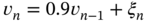 with
with  .
.
Now that we understand the need to modify the KF for colored and correlated noise, we can do it from a more general point of view than for the standard KF and come up with a universal linear algorithm called general Kalman filter (GKF) [185], which can have various forms. Evidence for the better performance of the GKF, even a minor improvement, can be found in many works, since white noise is unrealistic.
In many cases, the dynamics of CMN ![]() and colored process noise (CPN)
and colored process noise (CPN) ![]() can be viewed as Gauss‐Markov processes, which complement the state‐space model as
can be viewed as Gauss‐Markov processes, which complement the state‐space model as
where ![]() and
and ![]() are the covariances of white Gaussian noise vectors
are the covariances of white Gaussian noise vectors ![]() and
and ![]() and cross‐covariances
and cross‐covariances ![]() and
and ![]() represent the time‐correlation between
represent the time‐correlation between ![]() and
and ![]() . Equations 3.98 and (3.99) suggest that the coloredness factors
. Equations 3.98 and (3.99) suggest that the coloredness factors ![]() and
and ![]() should be chosen so that
should be chosen so that ![]() and
and ![]() remain stationary. Since the model (3.97)–(3.100) is still linear with white Gaussian
remain stationary. Since the model (3.97)–(3.100) is still linear with white Gaussian ![]() and
and ![]() , the Kalman approach can be applied and the GKF derived in the same way as KF.
, the Kalman approach can be applied and the GKF derived in the same way as KF.
Two approaches have been developed for applying KF to (3.97)–(3.100). The first augmented states approach was proposed by A. E. Bryson et al. in [24,25] and is the most straightforward. It proposes to combine the dynamic equations 3.97–(3.99) into a single augmented state equation and represent the model as

where  . Obviously, the augmented equations 3.101 and (3.102) can be easily simplified to address only CPN, CMN, or noise correlation problems. An easily seen drawback is that the observation equation 3.102 has zero measurement noise. This makes it impossible to apply some KF versions that require inversion of the covariance matrix
 ![]() , such as information KF and alternate KF form. Therefore, the KF is said to be ill conditioned for state augmentation [25].
, such as information KF and alternate KF form. Therefore, the KF is said to be ill conditioned for state augmentation [25].
The second approach, which avoids the state augmentation, was proposed and developed by A. E. Bryson et al. in [24,25] and is now known as Bryson's algorithm. This algorithm was later improved in [147] to what is now referred to as the Petovello algorithm. The idea was to use measurement differencing to convert the model with CMN to a standard model with new matrices, but with white noise. The same idea was adopted in [182] for systems with CPN using state differencing. Next, we show several GKF algorithms for time‐correlated and colored noise sources.
Time‐Correlated Noise
If noise has a very short correlation time compared to time intervals of interest, it is typically considered as white and its coloredness can be neglected. Otherwise, system may experience a great noise interference [58].
When the noise sources are white, ![]() and
and ![]() , but time correlated with
, but time correlated with ![]() , equations 3.98 and (3.99) can be ignored, and (3.101) and (3.102) return to their original forms (3.32) and (3.33) with time‐correlated
, equations 3.98 and (3.99) can be ignored, and (3.101) and (3.102) return to their original forms (3.32) and (3.33) with time‐correlated ![]() and
and ![]() . There are two ways to apply KF for time‐correlated
. There are two ways to apply KF for time‐correlated ![]() and
and ![]() . We can either de‐correlate
. We can either de‐correlate ![]() and
and ![]() or derive a new bias correction gain (Kalman gain) to guarantee the filter optimality.
or derive a new bias correction gain (Kalman gain) to guarantee the filter optimality.
Noise de‐correlation. To de‐correlate ![]() and
and ![]() and thereby make it possible to apply KF, one can use the Lagrange method [15] and combine (3.32) with the term
and thereby make it possible to apply KF, one can use the Lagrange method [15] and combine (3.32) with the term ![]() , where
, where ![]() is a data vector and the Lagrange multiplier
is a data vector and the Lagrange multiplier ![]() is yet to be determined. This transforms the state equation to
is yet to be determined. This transforms the state equation to

where we assign
and white noise ![]() has the covariance
has the covariance ![]() ,
,

To find a matrix ![]() such that
such that ![]() and
and ![]() become uncorrelated, the natural statement
become uncorrelated, the natural statement ![]() leads to
leads to
and the Lagrange multiplier can be found as
Finally, replacing in (3.107) the product ![]() taken from (3.108) removes
taken from (3.108) removes ![]() , and (3.107) becomes
, and (3.107) becomes

Given ![]() ,
, ![]() ,
, ![]() ,
, ![]() ,
, ![]() , and
, and ![]() , the GKF estimates can be updated using Algorithm 1, in which
, the GKF estimates can be updated using Algorithm 1, in which ![]() should be substituted with
should be substituted with ![]() (3.110) using
(3.110) using ![]() given by (3.109) and
given by (3.109) and ![]() with
with ![]() (3.105). We thus have
(3.105). We thus have
where ![]() is given by (3.104).
is given by (3.104).
New Kalman gain. Another possibility to apply KF to models with time‐correlated ![]() and
and ![]() implies obtaining a new Kalman gain
implies obtaining a new Kalman gain ![]() . In this case, first it is necessary to change the error covariance (3.76) for correlated
. In this case, first it is necessary to change the error covariance (3.76) for correlated ![]() and
and ![]() as
as

where ![]() is given by (3.74) and
is given by (3.74) and ![]() by (3.77). Using (A.3) and (A.6), the derivative of the trace of
by (3.77). Using (A.3) and (A.6), the derivative of the trace of ![]() with respect to
with respect to ![]() can be found as
can be found as
By equating the derivative to zero, ![]() , we can find the optimal Kalman gain as
, we can find the optimal Kalman gain as
and notice that it becomes the original gain (3.78) for uncorrelated noise, ![]() . Finally, (3.118) simplifies the error covariance (3.117) to
. Finally, (3.118) simplifies the error covariance (3.117) to
Given ![]() ,
, ![]() ,
, ![]() ,
, ![]() ,
, ![]() , and
, and ![]() , the GKF algorithm for time‐correlated
, the GKF algorithm for time‐correlated ![]() and
and ![]() becomes
becomes
As can be seen, when the correlation is removed by ![]() , the algorithm (3.120)–(3.125) becomes the standard KF Algorithm 1. It is also worth noting that the algorithms (3.111)–(3.116) and (3.120)–(3.125) produce equal estimates and, thus, they are identical with no obvious advantages over each other. We will see shortly that the corresponding algorithms for CMN are also identical.
, the algorithm (3.120)–(3.125) becomes the standard KF Algorithm 1. It is also worth noting that the algorithms (3.111)–(3.116) and (3.120)–(3.125) produce equal estimates and, thus, they are identical with no obvious advantages over each other. We will see shortly that the corresponding algorithms for CMN are also identical.
Colored Measurement Noise
The suggestion that CMN may be of Markov origin was originally made by Bryson et al. in [24] for continuous‐time and in [25] for discrete‐time tracking systems. Two fundamental approaches have also been proposed in [25] for obtaining GKF for CMN: state augmentation and measurement differencing. The first approach involves reassigning the state vector so that the white sources are combined in an augmented system noise vector. This allows using KF directly, but makes it ill‐conditioned, as shown earlier. Even so, state augmentation is considered to be the main solution to the problem caused by CMN [54,58,185].
For CMN, the state‐space equations can be written as
where ![]() and
and ![]() are zero mean white Gaussian with the covariances
are zero mean white Gaussian with the covariances ![]() and
and ![]() and the property
and the property ![]() for all
for all ![]() and
and ![]() . Augmenting the state vector gives
. Augmenting the state vector gives

where, as in (3.101), zero observation noise makes KF ill‐conditioned.
To avoid increasing the state vector, one can apply the measurement differencing approach [25] and define a new observation ![]() as
as
By substituting ![]() taken from (3.126) and
taken from (3.126) and ![]() taken from (3.127), the observation equation 3.129 becomes
taken from (3.127), the observation equation 3.129 becomes
where we introduced
![]() , and white noise
, and white noise ![]() with the properties
with the properties
where
Now the modified model (3.126) and (3.130) contains white and time‐correlated noise sources ![]() and
and ![]() , for which the prior estimate
, for which the prior estimate ![]() is defined by (3.70) and the prior error covariance
is defined by (3.70) and the prior error covariance ![]() by (3.74).
by (3.74).
For (3.130), the measurement residual can be written as
and the innovation covariance ![]() can be transformed as
can be transformed as

The recursive GKF estimate can thus be written as

where the Kalman gain ![]() should be found for either time‐correlated or de‐correlated
should be found for either time‐correlated or de‐correlated ![]() and
and ![]() . Thereby, one can come up with two different, although mathematically equivalent, algorithms as discussed next.
. Thereby, one can come up with two different, although mathematically equivalent, algorithms as discussed next.
Correlated noise. For time‐correlated ![]() and
and ![]() , KF can be applied if we find the Kalman gain
, KF can be applied if we find the Kalman gain ![]() by minimizing the trace of the error covariance
by minimizing the trace of the error covariance ![]() . Representing the estimation error
. Representing the estimation error ![]() with
with
and noticing that ![]() does not correlate
does not correlate ![]() and
and ![]() , we obtain the error covariance
, we obtain the error covariance ![]() as
as


where ![]() is given by (3.120) and
is given by (3.120) and ![]() by (3.139).
by (3.139).
Now the optimal Kalman gain ![]() can be found by minimizing
can be found by minimizing ![]() using (A.3), (A.4), and (A.6). Equating to zero the derivative of
using (A.3), (A.4), and (A.6). Equating to zero the derivative of ![]() with respect to
with respect to ![]() gives
gives

and we obtain
Finally, replacing the first component in the last term in (3.142b) with (3.144) gives
Given ![]() ,
, ![]() ,
, ![]() ,
, ![]() ,
, ![]() , and
, and ![]() , the GKF equations become [183]
, the GKF equations become [183]
and we notice that ![]() causes
causes ![]() ,
, ![]() ,
, ![]() , and
, and ![]() , and this algorithm converts to the standard KF Algorithm 1.
, and this algorithm converts to the standard KF Algorithm 1.
De‐correlated noise. Alternatively, efforts can be made to de‐correlate ![]() and
and ![]() by repeating steps (3.103)–(3.110) as shown next. Similarly to (3.103), rewrite the state equation as
by repeating steps (3.103)–(3.110) as shown next. Similarly to (3.103), rewrite the state equation as

where the following variables are assigned
and require that noise ![]() be white with the covariance
be white with the covariance
Matrix ![]() that makes
that makes ![]() and
and ![]() uncorrelated can be found by representing
uncorrelated can be found by representing ![]() with
with
that gives the following Lagrange multiplier
Substituting ![]() taken from (3.157) into the last term in (3.156) removes
taken from (3.157) into the last term in (3.156) removes ![]() and (3.156) takes the form
and (3.156) takes the form
Given ![]() ,
, ![]() ,
, ![]() ,
, ![]() ,
, ![]() , and
, and ![]() , the GKF equations become [183]
, the GKF equations become [183]
Again we notice that ![]() makes
makes ![]() ,
, ![]() ,
, ![]() ,
, ![]() ,
, ![]() , and
, and ![]() , and this algorithm transforms to KF Algorithm 1. Next, we will show that algorithms (3.146)–(3.151) and (3.160)–(3.165) give identical estimates and therefore are equivalent.
, and this algorithm transforms to KF Algorithm 1. Next, we will show that algorithms (3.146)–(3.151) and (3.160)–(3.165) give identical estimates and therefore are equivalent.
Equivalence of GKF Algorithms for CMN
The equivalence of the Bryson and Petovello algorithms for CMN was shown in [33], assuming time‐invariant noise covariances that do not distinguish between FE‐ and BE‐based models. We will now show that the GKF algorithms (3.146)–(3.151) and (3.160)–(3.165) are also equivalent [183]. Note that the algorithms can be said to be equivalent in the MSE sense if they give the same estimates for the same input; that is, for the given ![]() and
and ![]() , the outputs
, the outputs ![]() and
and ![]() in both algorithms are identical.
in both algorithms are identical.
First, we represent the prior estimate ![]() (3.163) via the prior estimate
(3.163) via the prior estimate ![]() (3.149) and the prior error covariance
(3.149) and the prior error covariance ![]() (3.160) via
(3.160) via ![]() (3.146) as
(3.146) as


where ![]() . We now equate estimates (3.150) and (3.164),
. We now equate estimates (3.150) and (3.164),
substitute (3.166), combine with (3.153), transform as
and skip the nonzero equal terms from the both sides. This relates the gains ![]() and
and ![]() as
as
which is the main condition for both estimates to be identical.
If also (3.168) makes the error covariances identical, then the algorithms can be said to be equivalent. To make sure that this is the case, we equate (3.151) and (3.165) as
substitute (3.168) and (3.167), rewrite (3.169) as

introduce ![]() , and arrive at
, and arrive at

By rearranging the terms, this relationship can be transformed into

and, by substituting ![]() , represented with
, represented with
which, after tedious manipulations with matrices, becomes

By substituting ![]() taken from
taken from ![]() , we finally end up with
, we finally end up with
Because ![]() is symmetric,
is symmetric, ![]() , and (3.131) means
, and (3.131) means ![]() , then it follows that (3.171) is the equality
, then it follows that (3.171) is the equality ![]() , and we conclude that the algorithms (3.146)–(3.151) and (3.160)–(3.165) are equivalent. It can also be shown that they do not demonstrate significant advantages over each other.
, and we conclude that the algorithms (3.146)–(3.151) and (3.160)–(3.165) are equivalent. It can also be shown that they do not demonstrate significant advantages over each other.
Colored Process Noise
Process noise becomes colored for various reasons, often when the internal control mechanism is not reflected in the state equation and thus becomes the error component. For example, the IEEE Standard 1139‐2008 [75] states that, in addition to white noise, the oscillator phase PSD has four independent CPNs with slopes ![]() ,
, ![]() ,
, ![]() , and
, and ![]() , where f is the Fourier frequency. Unlike CMN, which needs to be filtered out, slow CPN behavior can be tracked, as in localization and navigation. But when solving the identification problem, both the CMN and the CPN are commonly removed. This important feature distinguishes GKFs designed for CMN and CPN.
, where f is the Fourier frequency. Unlike CMN, which needs to be filtered out, slow CPN behavior can be tracked, as in localization and navigation. But when solving the identification problem, both the CMN and the CPN are commonly removed. This important feature distinguishes GKFs designed for CMN and CPN.
A linear process with CPN can be represented in state space in the standard formulation of the Gauss‐Markov model with the equations
where ![]() ,
, ![]() ,
, ![]() , and
, and ![]() . To obtain GKF for CPN, we assign
. To obtain GKF for CPN, we assign ![]() ,
, ![]() , and
, and ![]() , and think that
, and think that ![]() ,
, ![]() , and
, and ![]() are nonsingular. We also suppose that the noise vectors
are nonsingular. We also suppose that the noise vectors ![]() and
and ![]() are uncorrelated with the covariances
are uncorrelated with the covariances ![]() and
and ![]() , and choose the matrix
, and choose the matrix ![]() so that CPN
so that CPN ![]() remains stationary.
remains stationary.
The augmented state‐space model for CPN becomes

and we see that, unlike (3.101), this does not make the KF ill‐conditioned. On the other hand, colored noise ![]() repeated in the state
repeated in the state ![]() can cause extra errors in the KF output under certain conditions.
can cause extra errors in the KF output under certain conditions.
To avoid the state augmentation, we now reason similarly to the measurement differencing approach [25] and derive the GKF for CPN based on the model (3.172)–(3.174) using the state differencing approach [182].
Using the state differencing method, the new state ![]() can be written as
can be written as
where ![]() ,
, ![]() ,
, ![]() , and
, and ![]() are still to be determined. The KF can be applied if we rewrite the new state equation as
are still to be determined. The KF can be applied if we rewrite the new state equation as
and find the conditions under which the noise ![]() will be zero mean and white Gaussian,
will be zero mean and white Gaussian, ![]() . By referring to (3.176), unknown variables can be retrieved by putting to zero the remainder in (3.175b),
. By referring to (3.176), unknown variables can be retrieved by putting to zero the remainder in (3.175b),
Then we replace ![]() taken from (3.175a) into (3.177), combine with
taken from (3.175a) into (3.177), combine with ![]() taken from (3.172), and write
taken from (3.172), and write

Although ![]() may hold for some applications, the case
may hold for some applications, the case ![]() for arbitrary
for arbitrary ![]() is isolated, and a solution to (3.178) can thus be found with simultaneous solution of four equations
is isolated, and a solution to (3.178) can thus be found with simultaneous solution of four equations
which suggest that the modified control signal ![]() is given by (3.180), and for nonsingular
is given by (3.180), and for nonsingular ![]() ,
, ![]() , and
, and ![]() (3.181) gives
(3.181) gives
where ![]() is a weighted version of
is a weighted version of ![]() . Next, substituting (3.183) into (3.179) and providing some transformations give the backward and forward recursions for
. Next, substituting (3.183) into (3.179) and providing some transformations give the backward and forward recursions for ![]() ,
,

It can be seen that ![]() becomes
becomes ![]() for white noise if
for white noise if ![]() and
and ![]() , which follows from the backward recursion (3.184), but is not obvious from the forward recursion (3.185).
, which follows from the backward recursion (3.184), but is not obvious from the forward recursion (3.185).
What follows is that the choice of the initial ![]() is critical to run (3.185). Indeed, if we assume that
is critical to run (3.185). Indeed, if we assume that ![]() , then (3.185) gives
, then (3.185) gives ![]() , which may go far beyond the proper matrix. But for the diagonal
, which may go far beyond the proper matrix. But for the diagonal ![]() with equal components
with equal components ![]() is the only solution. On the other hand,
is the only solution. On the other hand, ![]() gives
gives ![]() , which makes no sense. One way to specify
, which makes no sense. One way to specify ![]() is to assume that the process is time‐invariant up to
is to assume that the process is time‐invariant up to ![]() , convert (3.184) to the nonsymmetric algebraic Riccati equation (NARE) [107] or quadratic matrix equation
, convert (3.184) to the nonsymmetric algebraic Riccati equation (NARE) [107] or quadratic matrix equation
and solve (3.186) for ![]() . However, the solution to (3.186) is generally not unique [107], and efforts must be made to choose the proper one.
. However, the solution to (3.186) is generally not unique [107], and efforts must be made to choose the proper one.
So the modified state equation 3.176 becomes
with white Gaussian ![]() and matrix
and matrix ![]() , which is obtained recursively using (3.185) for the properly chosen fit
, which is obtained recursively using (3.185) for the properly chosen fit ![]() of (3.186). To specify the initial
of (3.186). To specify the initial ![]() , we consider (3.175a) at
, we consider (3.175a) at ![]() and write
and write ![]() . Since
. Since ![]() is not available, we set
is not available, we set ![]() and take
and take ![]() as a reasonable initial state to run (3.187).
as a reasonable initial state to run (3.187).
Finally, extracting ![]() from (3.175a), substituting it into the observation equation 3.174, and rearranging the terms, we obtain the modified observation equation
from (3.175a), substituting it into the observation equation 3.174, and rearranging the terms, we obtain the modified observation equation
with respect to ![]() , in which
, in which ![]() can be replaced by the estimate
can be replaced by the estimate ![]() .
.
Given ![]() ,
, ![]() ,
, ![]() ,
, ![]() ,
, ![]() , and
, and ![]() , the GKF equations for CPN become
, the GKF equations for CPN become
A specific feature of this algorithm is that the future values of ![]() and
and ![]() are required at
are required at ![]() , which is obviously not a problem for LTI systems. It is also seen that
, which is obviously not a problem for LTI systems. It is also seen that ![]() results in
results in ![]() and
and ![]() , and the algorithm becomes the standard KF Algorithm 1.
, and the algorithm becomes the standard KF Algorithm 1.
3.2.9 Kalman‐Bucy Filter
The digital world today requires fast and accurate digital state estimators. But when the best sampling results in significant loss of information due to limitations in the operation frequency of digital devices, then there will be no choice but to design and implement filters physically in continuous time.
The optimal filter for continuous‐time stochastic linear systems was obtained in [85] by Kalman and Bucy and is called the Kalman‐Bucy filter (KBF). Obtaining KBF can be achieved in a standard way by minimizing MSE. Another way is to convert KF to continuous time as shown next.
Consider a stochastic LTV process represented in continuous‐time state space by the following equations
where the initial ![]() is supposed to be known.
is supposed to be known.
For a sufficiently short time interval ![]() , we can assume that all matrices and input signal are piecewise constant when
, we can assume that all matrices and input signal are piecewise constant when ![]() and take
and take ![]() ,
, ![]() ,
, ![]() , and
, and ![]() . Following (3.6) and assuming that
. Following (3.6) and assuming that ![]() is small, we can then approximate
is small, we can then approximate ![]() with
with ![]() and write the solution to (3.196) as
and write the solution to (3.196) as

Thus, the discrete analog of model (3.196) and (3.197) is
where we take ![]() ,
,

refer to (3.25) and (3.26), and define the noise covariances as ![]() and
and ![]() , where
, where ![]() is the PSD of
is the PSD of ![]() and
and ![]() is the PSD of
is the PSD of ![]() . Ensured correspondence between continuous‐time model (3.196) and (3.197) and discrete‐time model (3.198) and (3.199) for small
. Ensured correspondence between continuous‐time model (3.196) and (3.197) and discrete‐time model (3.198) and (3.199) for small ![]() , the KBF can be obtained as follows.
, the KBF can be obtained as follows.
We first notice that the continuous time estimate does not distinguish between the prior and posterior estimation errors due to ![]() . Therefore, the optimal Kalman gain
. Therefore, the optimal Kalman gain ![]() (3.78) for small
(3.78) for small ![]() can be transformed as
can be transformed as

where ![]() is the optimal Kalman gain in continuous time.
is the optimal Kalman gain in continuous time.
The Kalman estimate (3.72) can now be transformed for small ![]() as
as

where ![]() is given by (3.201).
is given by (3.201).
Reasoning along similar lines as for (3.201), error covariance ![]() (3.79) combined with
(3.79) combined with ![]() , defined as (3.75), can also be transformed for small
, defined as (3.75), can also be transformed for small ![]() as
as
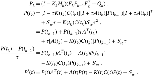
where (3.203) is the Riccati differential equation (RDE) (A.25).
Thus, the KBF can be represented by two differential equations

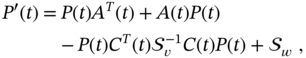
given the initial state ![]() and error covariance
and error covariance ![]() .
.
It is worth noting that although less attention is paid to the RBP in the modern digital world, its hardware implementation is required when the main spectral information is located above the operation frequency of the digital device.
3.3 Linear Recursive Smoothing
When better noise reduction is required than using optimal filtering, we think of optimal smoothing. The term smoothing comes from antiquity, and solutions to the smoothing problem can be found in the works of Gauss, Kolmogorov, and Wiener. Both optimal filtering and optimal smoothing minimize the MSE using data taken from the past up to the current time index ![]() . What distinguishes the two approaches is that optimal filtering gives an estimate in the current time index
. What distinguishes the two approaches is that optimal filtering gives an estimate in the current time index ![]() , while optimal smoothing refers the estimate to the past point
, while optimal smoothing refers the estimate to the past point ![]() with a lag
with a lag ![]() . Therefore, it is common to say that
. Therefore, it is common to say that ![]() is the output of an optimal filter and
is the output of an optimal filter and ![]() is the output of a
is the output of a ![]() ‐lag optimal smoother. Smoothing can also be organized at the current point
‐lag optimal smoother. Smoothing can also be organized at the current point ![]() by involving
by involving ![]() future data. In this case, it is said that the estimate
future data. In this case, it is said that the estimate ![]() is produced by a
is produced by a ![]() ‐lag smoothing filter.
‐lag smoothing filter.
The following smoothing problems can be solved:
- Fixed‐lag smoothing gives an estimate at
 with a fixed lag
  over a horizon
  , where
  can be zero.
 - Fixed‐interval smoothing gives an estimate at any point in a fixed interval
 with a lag
  ranging from
  to
to  .
. - Fixed‐point smoothing gives an estimate at a fixed point
 in
in  with variable lag
  , where
  can be zero.
The opposite problem to smoothing is called prediction. The prediction refers to an estimate of the future point with some step ![]() , and it is said that
, and it is said that ![]() is the
is the ![]() ‐step predictive estimate and
‐step predictive estimate and ![]() is the
is the ![]() ‐step predictive filtering estimate.
‐step predictive filtering estimate.
Several two‐pass (forward‐backward) smoothers have been developed using Kalman recursions [9,83]. The idea behind each such solution is to provide forward filtering using KF and then arrange the backward pass to obtain a ![]() ‐lag smoothing estimate at
‐lag smoothing estimate at ![]() . Next we will look at a few of the most widely used recursive smoothers.
. Next we will look at a few of the most widely used recursive smoothers.
3.3.1 Rauch‐Tung‐Striebel Algorithm
In the Rauch‐Tung‐Striebel (RTS) smoother developed for fixed intervals [154], the forward state estimates ![]() and
and ![]() and the error covariances
and the error covariances ![]() and
and ![]() are taken at each
are taken at each ![]() from KF, and then the
from KF, and then the ![]() ‐lag smoothed state estimate
‐lag smoothed state estimate ![]() and error covariance
and error covariance ![]() are computed at
are computed at ![]() backward using backward recursions.
backward using backward recursions.
If we think of a smoothing estimate ![]() as an available filtering estimate
as an available filtering estimate ![]() adjusted for the predicted residual
adjusted for the predicted residual ![]() by the gain
by the gain ![]() as
as
then the RTS smoother derivation can be provided as follows.
Define the smoother error ![]() by
by
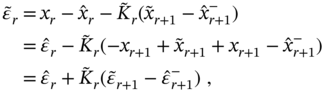
which gives the error covariance
To find the optimal smoother gain ![]() , substitute
, substitute ![]() , represent (3.107) as
, represent (3.107) as

and arrive at another form of the error covariance
Now, apply the derivative with respect to ![]() to the trace of
to the trace of ![]() , consider
, consider ![]() as the process noise covariance
as the process noise covariance ![]() , and obtain
, and obtain ![]() . The RTS smoothing algorithm can then be formalized with the following steps,
. The RTS smoothing algorithm can then be formalized with the following steps,
where the required KF estimates ![]() ,
, ![]() ,
, ![]() , and
, and ![]() must be available (saved) from the filtering procedure. A more complete analysis of RTS smoother can be found in [83,185].
must be available (saved) from the filtering procedure. A more complete analysis of RTS smoother can be found in [83,185].
3.3.2 Bryson‐Frazier Algorithm
Another widely used modified Bryson‐Frazier (MBF) smoother, developed by Bierman [20] for fixed intervals, also uses data stored from the KF forward pass. In this algorithm, the backward pass for ![]() and
and ![]() is organized using the following recursions,
is organized using the following recursions,
where ![]() and other definitions are taken from Algorithm 4. The MBF
and other definitions are taken from Algorithm 4. The MBF ![]() ‐lag smoothing estimate and error covariance are then found as
‐lag smoothing estimate and error covariance are then found as
It can be seen that the inversion of the covariance matrix is not required for this algorithm, which is an important advantage over the RTS algorithm.
3.3.3 Two‐Filter (Forward‐Backward) Smoothing
Another solution to the smoothing problem can be proposed if we consider data on ![]() , where
, where ![]() can be zero, provide forward filtering on
can be zero, provide forward filtering on ![]() and backward filtering on
and backward filtering on ![]() , and then combine both estimates at
, and then combine both estimates at ![]() . The resulting two‐filter (or forward‐backward) smoother is suitable for the fixed interval problem [83], but can also be applied to other smoothing problems. Furthermore, both recursive and batch structures can be designed for two‐filter smoothing by fusing either filtering or predictive estimates.
. The resulting two‐filter (or forward‐backward) smoother is suitable for the fixed interval problem [83], but can also be applied to other smoothing problems. Furthermore, both recursive and batch structures can be designed for two‐filter smoothing by fusing either filtering or predictive estimates.
A two‐filter smoother can be designed if we assume that the forward filtering estimate is obtained at ![]() over
over ![]() as
as ![]() and the backward filtering estimate is obtained at
and the backward filtering estimate is obtained at ![]() over
over ![]() as
as ![]() . The smoothing estimate
. The smoothing estimate ![]() can then be obtained by combining both estimates as
can then be obtained by combining both estimates as
where the gains ![]() and
and ![]() are required such that the MSE is minimized for the optimal
are required such that the MSE is minimized for the optimal ![]() . Since
. Since ![]() and
and ![]() should not cause a regular error (bias), they can be linked as
should not cause a regular error (bias), they can be linked as ![]() . Then (3.218) can be represented as
. Then (3.218) can be represented as
By defining the forward filtering error as ![]() , the backward one as
, the backward one as ![]() , and the smoother error as
, and the smoother error as ![]() , we next represent the error covariance
, we next represent the error covariance ![]() as
as
equate to zero the derivative applied to the trace of ![]() with respect to
with respect to ![]() , and obtain the optimal gains as
, and obtain the optimal gains as
Using (3.220) and (3.221), the error covariance ![]() can finally be transformed to
can finally be transformed to
and we see that the information ![]() about the smoothing estimate (3.219) is additively combined with the information
about the smoothing estimate (3.219) is additively combined with the information ![]() at the output of the forward filter and
at the output of the forward filter and ![]() at the output of the backward filter,
at the output of the backward filter,
The proof of (3.222) can be found in [83,185] and is postponed to “Problems”.
Thus, two‐filter (forward‐backward) smoothing is provided by (3.218) with optimal gains (3.220) and (3.221) and error covariance (3.222). It also follows that the information identity (3.223) is fundamental to two‐filter optimal smoothing and must be obeyed regardless of structure (batch or recursive). Practical algorithms of these smoothers are given in [185], and more details about the two‐filter smoothing problem can be found in [83].
3.4 Nonlinear Models and Estimators
So far, we have looked at linear models and estimators. Since many systems are nonlinear in nature and therefore have nonlinear dynamics, their mathematical representations require nonlinear ODEs [80] and algebraic equations. More specifically, we will assume that the process (or system) is nonlinear and that measurement can also be provided using nonlinear sensors. For white Gaussian noise, the exact solution of the nonlinear problem in continuous time was found by Stratonovich [193] and Kushner [92] in the form of a stochastic partial differential equation (SPDE). The state probability density associated with the SPDE is given by the Stratonovich‐Kushner equation, which belongs to the FPK family of equations (2.118), and KBF is its particular solution. Because the Stratonovich‐Kuchner equation has no general solution and is therefore impractical in discrete time, much more attention has been drawn to approximate solutions developed during decades to provide a state estimate with sufficient accuracy.
In discrete‐time state‐space, the nonlinear state and observation equations can be written, respectively, as
where ![]() and
and ![]() are some nonlinear time‐varying functions,
are some nonlinear time‐varying functions, ![]() is an input, and
is an input, and ![]() and
and ![]() are white Gaussian with known statistics. If the noise is of low intensity or acts additively, the model (3.224) and (3.225) is often written as
are white Gaussian with known statistics. If the noise is of low intensity or acts additively, the model (3.224) and (3.225) is often written as
Provided the posterior distribution ![]() of the state
of the state ![]() by (3.39), the Bayesian estimate
by (3.39), the Bayesian estimate ![]() for nonlinear models can be found as (3.41) with error covariance (3.42). For Gauss‐Markov processes,
for nonlinear models can be found as (3.41) with error covariance (3.42). For Gauss‐Markov processes, ![]() can be specified by solving the FPK equation (2.118) in the stationary mode as (2.120). This gives fairly accurate estimates, but in practice difficulties arise when
can be specified by solving the FPK equation (2.118) in the stationary mode as (2.120). This gives fairly accurate estimates, but in practice difficulties arise when ![]() and/or
and/or ![]() are not smooth enough and the noise is large.
are not smooth enough and the noise is large.
To find approximate solutions, Cox in [38] and others extended KF to nonlinear models in the first‐order approximation, and Athans, Wishner, and Bertolini provided it in [12] in the second‐order approximation. However, it was later told [178,185] that nothing definite can be said about the second‐order approximation, and the first‐order extended KF (EKF) was recommended as the main tool. Yet another versions of EKF have been proposed, such as the divided difference filter [136] and quadrature KF [10], and we notice that several solutions beyond the EKF can be found in [40].
Referring to particularly poor performance of the EKF when the system is highly nonlinear and noise large [49], Julier, Uhlmann, and Durrant‐Whyte developed the unscented KF (UKF) [81,82,199] to pick samples around the mean, propagate through the nonlinearity, and then recover the mean and covariance. Although the UKF often outperforms the EKF and can be improved by using high‐order statistics, it loses out in many applications to another approach known as particle filtering.
The idea behind the particle filter (PF) approach [44] is to use sequential Monte Carlo (MC) methods [116] and solve the filtering problem by computing the posterior distributions of the states of some Markov process, given some noisy and partial observations. Given enough time to generate a large number of particles, the PF usually provides better accuracy than other nonlinear estimators. Otherwise, it can suffer from two effects called sample degeneracy and sample impoverishment, which cause divergence.
Next we will discuss the most efficient nonlinear state estimators. Our focus will be on algorithmic solutions, advantages, and drawbacks.
3.4.1 Extended Kalman Filter
The EKF is viewed in state estimation as a nonlinear version of KF that linearizes the mean and covariance between two neighboring discrete points. For smooth rather than harsh nonlinearities, EKF has become the de facto standard technique used in many areas of system engineering.
For the model in (3.226) and (3.227), the first‐order EKF (EKF‐1) and the second‐order EKF (EKF‐2) can be obtained using the Taylor series as shown next. Suppose that both ![]() and
and ![]() are smooth functions and approximate them on a time step between two neighboring discrete points using the second‐order Taylor series. For simplicity, omit the known input
are smooth functions and approximate them on a time step between two neighboring discrete points using the second‐order Taylor series. For simplicity, omit the known input ![]() .
.
The nonlinear function ![]() can be expanded around the estimate
can be expanded around the estimate ![]() and
and ![]() around the prior estimate
around the prior estimate ![]() as [178]
as [178]
where the Jacobian matrices (A.20) are

![]() is the prior estimation error, and
is the prior estimation error, and ![]() is the estimation error. The second‐order terms are represented by [15]
is the estimation error. The second‐order terms are represented by [15]


where the Hessian matrices (A.21) are


and ![]() ,
, ![]() , and
, and ![]() ,
, ![]() , are the
, are the ![]() th and
th and ![]() th components, respectively, of vectors
th components, respectively, of vectors ![]() and
and ![]() . Also,
. Also, ![]() and
and ![]() are Cartesian basis vectors with the
are Cartesian basis vectors with the ![]() th and
th and ![]() th components equal to unity and all others equal to zero.
th components equal to unity and all others equal to zero.
Referring to (3.228) and (3.229), the nonlinear model (3.226) and (3.227) can now be approximated with
where the modified observation vector is ![]() , also
, also
and other matrices are specified earlier. As can be seen, the second‐order terms ![]() and
and ![]() affect only
affect only ![]() and
and ![]() . If
. If ![]() and
and ![]() contribute insignificantly to the estimates [185], they are omitted in the EKF‐1. Otherwise, the second‐order EKF‐2 is used.
contribute insignificantly to the estimates [185], they are omitted in the EKF‐1. Otherwise, the second‐order EKF‐2 is used.
The EKF algorithm can now be summarized with the recursions
Now it is worth mentioning again that the EKF usually works very accurately when both nonlinearities are weak. However, if this condition is not met and the nonlinearity is severe, another approach using the “unscented transformation” typically gives better estimates. The corresponding modification of the KF [81] is considered next.
3.4.2 Unscented Kalman Filter
Referring to typically large errors and possible divergence of the KF with sharp nonlinearities [49], Julier, Uhlrnann, and Durrant‐Whyte have developed another approach to nonlinear filtering, following the intuition that it is easier to approximate a probability distribution than it is to approximate an arbitrary nonlinear function or transformation [82]. The approach originally proposed by Uhlrnann in [199] was called the unscented transformation (UT) and resulted in the unscented (or Uhlrnann) KF (UKF) [81,82]. The UKF has been further deeply investigated and used extensively in nonlinear filtering practice. Next we will succinctly introduce UT and UKF, referring the reader to [185] and many other books, tutorials, and papers discussing the theory and applications of UT and UKF for further learning.
The Unscented Transformation
Consider a nonlinear function ![]() . The problem with its linear approximation (3.210) is that the matrix
. The problem with its linear approximation (3.210) is that the matrix ![]() projects
projects ![]() into the next time index
into the next time index ![]() in a linear way, which may not be precise and even cause divergence. To avoid the linearization and not use matrix
in a linear way, which may not be precise and even cause divergence. To avoid the linearization and not use matrix ![]() , we can project through
, we can project through ![]() the statistics of
the statistics of ![]() and obtain at
and obtain at ![]() the mean and approximate covariance. First of all, we are interested in the projection of the mean and the deviations from the mean by the standard deviation.
the mean and approximate covariance. First of all, we are interested in the projection of the mean and the deviations from the mean by the standard deviation.
Referring to [82], we can consider a ![]() ‐state process and assign
‐state process and assign ![]() weighted samples of sigma points
weighted samples of sigma points ![]() at
at ![]() for
for ![]() as
as
where ![]() , and
, and ![]() means the
means the ![]() th column of
th column of ![]() if
if ![]() . Otherwise, if
. Otherwise, if ![]() ,
, ![]() means the
means the ![]() th raw of
th raw of ![]() . Note that, to find the matrix square root, the Cholesky decomposition method can be used [59]. A tuning factor
. Note that, to find the matrix square root, the Cholesky decomposition method can be used [59]. A tuning factor ![]() can be either positive or negative, although such that
can be either positive or negative, although such that ![]() . This factor is introduced to affect the fourth and higher‐order sample moments of the sigma points.
. This factor is introduced to affect the fourth and higher‐order sample moments of the sigma points.
While propagating through ![]() , the sigma points (3.245) are projected at
, the sigma points (3.245) are projected at ![]() as
as
and one may compute the predicted mean ![]() by the weighed sum of
by the weighed sum of ![]() as
as

where the weighted function ![]() is specified in [82] as
is specified in [82] as ![]() for
for ![]() and as
and as ![]() for
for ![]() . But it can also be chosen in another way, for example, as
. But it can also be chosen in another way, for example, as ![]() for
for ![]() and
and ![]() for
for ![]() [185]. The advantage of the UT approach is that the weights
[185]. The advantage of the UT approach is that the weights ![]() can be chosen in such a way that this also affects higher‐order statistics.
can be chosen in such a way that this also affects higher‐order statistics.
Provided ![]() by (3.247), the error covariance can be predicted as
by (3.247), the error covariance can be predicted as

Referring to (3.246) and ![]() in (3.227), the predicted observations can then be formed as
in (3.227), the predicted observations can then be formed as
and further averaged to obtain

with the prediction error covariance

The cross‐covariance between ![]() and
and ![]() can be found as
can be found as

It follows that the UT just described provides a set of statistics at the outputs of the nonlinear blocks for an optimal solution to the filtering problem. The undoubted advantage over the Taylor series (3.228) and (3.229) is that the Jacobian matrices are not used, and projections are obtained directly through nonlinear functions.
UKF Algorithm
So the ultimate goal of the UKF algorithm is to get rid of all matrices of the EKF algorithm (3.240)–(3.244) using the previous introduced projections. Let us show how to do it. Since (3.248) predicts the error covariance, we can approximate ![]() with
with ![]() , and since (3.251) predicts the innovation covariance (3.223), we can approximate
, and since (3.251) predicts the innovation covariance (3.223), we can approximate ![]() with
with ![]() . Then the product
. Then the product ![]() in (3.242) can be transformed to
in (3.242) can be transformed to ![]() defined by (3.252) as
defined by (3.252) as
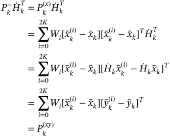
and the gain ![]() (3.242) represented as
(3.242) represented as ![]() . Finally, (3.244) can be transformed as
. Finally, (3.244) can be transformed as

It can be seen from the previous that there is now a complete set of predictions to get rid of matrices in EKF, and the UKF algorithm is thus the following
where ![]() is computed by (3.252),
is computed by (3.252), ![]() by (3.248),
by (3.248), ![]() by (3.251),
by (3.251), ![]() by (3.247), and
by (3.247), and ![]() by (3.250).
by (3.250).
Many studies have confirmed that the UKF in (3.255)–(3.257) is more accurate than EKF when the nonlinearity is not smooth. Moreover, using the additional degree of freedom ![]() in the weights
in the weights ![]() , the UKF can be made even more accurate. It should be noted, however, that the same statistics can be predicted by UT for different distributions, which is a serious limitation on accuracy. Next, we will consider the “particle filtering” approach that does not have this drawback.
, the UKF can be made even more accurate. It should be noted, however, that the same statistics can be predicted by UT for different distributions, which is a serious limitation on accuracy. Next, we will consider the “particle filtering” approach that does not have this drawback.
3.4.3 Particle Filtering
Along with the linear optimal KF, the Bayesian approach has resulted in two important suboptimal nonlinear solutions: point mass filter (PMF) [8] and particle filter (PF) [62]. The PMF computes posterior density recursively over a deterministic state‐space grid. It can be applied to any nonlinear and non‐Gaussian model, but it has a serious limitation: complexity. The PF performs sequential MC estimation by representing the posterior densities with samples or particles, similarly to PMF, and is generally more successful in accuracy than EKF and UKF for highly nonlinear systems with large Gaussian and non‐Gaussian noise.
To introduce the PF approach, we will assume that a nonlinear system is well represented by a first‐order Markov model and is observed over a nonlinear equation with (3.206) and (3.207) ignoring the input ![]() . We will be interested in the best estimate for
. We will be interested in the best estimate for ![]() , given measurements
, given measurements ![]() . More specifically, we will try to obtain a filtering estimate from
. More specifically, we will try to obtain a filtering estimate from ![]() . Within the Bayesian framework, the required estimate and the estimation error can be extracted from the conditional posterior probability density
. Within the Bayesian framework, the required estimate and the estimation error can be extracted from the conditional posterior probability density ![]() . This can be done, albeit approximately, using the classical “bootstrap” PF considered next.
. This can be done, albeit approximately, using the classical “bootstrap” PF considered next.
Bootstrap
The idea behind PF is simple and can be described in two steps, referring to the bootstrap proposed by Gordon, Salmond, and Smith [62].
Prediction. Draw ![]() samples3 (or particles)
samples3 (or particles) ![]() and
and ![]() . Pass these samples through the system model (3.206) to obtain
. Pass these samples through the system model (3.206) to obtain ![]() prior samples
prior samples ![]() . Since prediction may not be accurate, update the result next.
. Since prediction may not be accurate, update the result next.
Update. Using ![]() , evaluate the likelihood of each prior sample as
, evaluate the likelihood of each prior sample as ![]() , normalize by
, normalize by ![]() , and obtain a normalized weight
, and obtain a normalized weight ![]() , which is a discrete pmf over
, which is a discrete pmf over ![]() . From
. From ![]() , find the estimate of
, find the estimate of ![]() and evaluate errors. Optionally, resample
and evaluate errors. Optionally, resample ![]() times from
times from ![]() to generate samples
to generate samples ![]() such that
such that ![]() holds for any
holds for any ![]() .
.
If we generate a huge number of the particles at each ![]() , then the bootstrap will be as accurate as the best hypothetical filter. This, however, may not be suitable for many real‐time applications. But even if the computation time is not an issue, incorrectly set initial values cause errors in the bootstrap to grow at a higher rate than in the KF. Referring to these specifics, next we will consider a more elaborated and complete theory of PF.
, then the bootstrap will be as accurate as the best hypothetical filter. This, however, may not be suitable for many real‐time applications. But even if the computation time is not an issue, incorrectly set initial values cause errors in the bootstrap to grow at a higher rate than in the KF. Referring to these specifics, next we will consider a more elaborated and complete theory of PF.
Particle Filter Theory
Within the Bayesian framework, we are interested in the posterior pmf ![]() to obtain an estimate of
to obtain an estimate of ![]() and evaluate the estimation errors. Thus, we may suppose that the past
and evaluate the estimation errors. Thus, we may suppose that the past ![]() is known, although in practice it may be too brave.
is known, although in practice it may be too brave.
Assuming that ![]() is analytically inaccessible, we can find its discrete approximation at
is analytically inaccessible, we can find its discrete approximation at ![]() points as a function of
points as a function of ![]() . Using the sifting property of Dirac delta, we can also write
. Using the sifting property of Dirac delta, we can also write

and go to the discrete form by drawing samples ![]() from
from ![]() , which we think is not easy. But we can introduce the importance density
, which we think is not easy. But we can introduce the importance density ![]() , from which
, from which ![]() can easily be drawn. Of course, the importance density must be of the same class as
can easily be drawn. Of course, the importance density must be of the same class as ![]() , so it is pmf. At this point, we can rewrite (3.258) as
, so it is pmf. At this point, we can rewrite (3.258) as


where ![]() is defined by comparing (3.259a) and (3.259b). Since (3.259b) de facto is the expectation of
is defined by comparing (3.259a) and (3.259b). Since (3.259b) de facto is the expectation of ![]() , we then apply the sequential importance sampling (SIS), which is the MC method of integration, and rewrite (3.259b) in discrete form as
, we then apply the sequential importance sampling (SIS), which is the MC method of integration, and rewrite (3.259b) in discrete form as
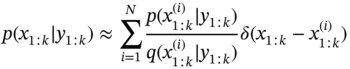

where the importance weight

corresponds to each of the generated particles ![]() . Note that (3.261) still needs to be normalized for
. Note that (3.261) still needs to be normalized for ![]() in order to be a density. Therefore, the sign
in order to be a density. Therefore, the sign ![]() is used.
is used.
To formalize the recursive form ![]() for (3.261), we apply Bayes' rule to
for (3.261), we apply Bayes' rule to ![]() and write
and write

Using ![]() and the Markov property, we next represent (3.262) as
and the Markov property, we next represent (3.262) as
Since the importance density is of the same class as ![]() , we follow [43,155], apply Bayes' rule to
, we follow [43,155], apply Bayes' rule to ![]() , and choose the importance density to factorize of the form
, and choose the importance density to factorize of the form
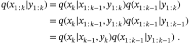
By combining (3.261), (3.263), and (3.264), the recursion for (3.261) can finally be found as
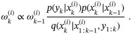
If we now substitute (3.265) in (3.260b), then we can use the density ![]() to find the Bayesian estimate
to find the Bayesian estimate
and the estimation error covariance

It should be noted that (3.266) and (3.267) are valid for both smoothing and filtering. In the case of filtering, the weight (3.265) ignores the past history and becomes
the posterior pmf (3.260b) transforms to
and the filtering estimates can be found as


Although PF is quite transparent and simple algorithmically, it has a serious drawback associated with the divergence caused by two effects called sample degeneracy and sample impoverishment [43,62,155]. Both these effects are associated with “bad” distribution of particles. The PF divergence usually occurs at low noise levels and is aggravated by incorrect initial values. There is a simple remedy for the divergency: set ![]() to make both (3.248) and (3.251) true densities. However, this causes computational problems in real‐time implementations.
to make both (3.248) and (3.251) true densities. However, this causes computational problems in real‐time implementations.
These disadvantages can be effectively overcome by improving the diversity of samples in hybrid structures [114]. Examples are the PF/UKF [201], PF/KF [43], and PF combined with the UFIR filter [143]. Nevertheless, none of the known solutions is protected from divergency when the noise is very low and ![]() is small. The following issues need to be addressed to improve the performance.
is small. The following issues need to be addressed to improve the performance.
Degeneracy. Obviously, the best choice of importance density is the posterior density itself. Otherwise, the unconditional variance of the importance weights increases with time for the observations ![]() , interpreted as random variables [43]. This unavoidable phenomenon, known as sample degeneracy [43], has the following practical appearance: after a few iterations, all but one of the normalized weights are very close to zero. Thus, a large computational load will be required to update the particles, whose contribution to the final estimate is almost zero.
, interpreted as random variables [43]. This unavoidable phenomenon, known as sample degeneracy [43], has the following practical appearance: after a few iterations, all but one of the normalized weights are very close to zero. Thus, a large computational load will be required to update the particles, whose contribution to the final estimate is almost zero.
Importance density. The wrong choice of importance density may crucially affect the estimate. Therefore, efforts should be made to justify acceptable solutions aimed at minimizing the variance of the importance weights.
Resampling. Resampling of particles is often required to reduce the effects of degeneracy. The idea behind resampling is to skip particles that have small weights and multiply ones with large weights. Although the resampling step mitigates the degeneracy, it poses another problem, which is discussed next.
Sample impoverishment. As a consequence of resampling, particles with large weights are statistically selected many times. It results in a loss of divergency between the particles, since the resulting sample will contain many repeated points. This problem is called sample impoverishment, and its effect can be especially destroying when the noise is low and the number of particles in insufficient.
3.5 Robust State Estimation
Robustness is required of an estimator when model errors occur due to mismodeling, noise environments are uncertain, and a system (process) undergoes unpredictable temporary changes such as jumps in velocity, phase, frequency, etc. Because the KF is poorly protected against such factors, efforts should be made whenever necessary to “robustify” the performance.
When a system is modeled with errors in poorly known noise environments, then matrices ![]() ,
, ![]() ,
, ![]() ,
, ![]() ,
, ![]() ,
, ![]() , and
, and ![]() in (3.32) and (3.33) can be complicated by uncertain additions
in (3.32) and (3.33) can be complicated by uncertain additions ![]() ,
, ![]() ,
, ![]() ,
, ![]() ,
, ![]() ,
, ![]() , and
, and ![]() , and the state‐space equations written as
, and the state‐space equations written as
where the covariance ![]() of noise
of noise ![]() and
and ![]() of
of ![]() may also have uncertain parts resulting in
may also have uncertain parts resulting in ![]() and
and ![]() .
.
Each uncertainty ![]() of a system can be completely or partially unknown, being either deterministic or stochastic [35]. But even if
of a system can be completely or partially unknown, being either deterministic or stochastic [35]. But even if ![]() is uncertain, the maximum values of its components are usually available in applications. This allows restricting the estimation error covariance, as was done by Toda and Patel in [197] for nonzero
is uncertain, the maximum values of its components are usually available in applications. This allows restricting the estimation error covariance, as was done by Toda and Patel in [197] for nonzero ![]() ,
, ![]() ,
, ![]() , and
, and ![]() . Minimizing errors for a set of maximized uncertain parameters, all of each have bounded norms, creates the foundation for robust filtering [65]. The robust state estimation problem also arises when all matrices are certain, but noise is not Gaussian, heavy‐tailed, or Gaussian with outliers.
. Minimizing errors for a set of maximized uncertain parameters, all of each have bounded norms, creates the foundation for robust filtering [65]. The robust state estimation problem also arises when all matrices are certain, but noise is not Gaussian, heavy‐tailed, or Gaussian with outliers.
The minimax approach is most popular in the design of robust estimators [87, 123, 124, 135, 207] under the previous assumptions. Shown that a saddle‐point property holds, the minimax estimator designed to have worst‐case optimal performance is referred to as minimax robust [160]. Huber showed in [73] that such an estimator can be treated as the ML estimator for the least favorable member of the class [160]. Referring to [73], several approaches have been developed over the decades to obtain various kinds of minimax state estimators, such as the robust KF and ![]() filter.
filter.
3.5.1 Robustified Kalman Filter
After leaving the comfortable Gaussian environment, the KF output degrades, and efforts must be made to improve performance. In many cases, this is easier to achieve by modifying the KF algorithm rather than deriving a new filter. For measurement noise with uncertain distribution (supposedly heavy‐tailed), Masreliez and Martin robustified KF [124] to protect against outliers in the innovation residual. To reduce errors caused by such an uncertainty, they introduced a symmetric vector influence function ![]() , where
, where ![]() is the weighted residual and
is the weighted residual and ![]() is a transformation matrix of a certain type. For
is a transformation matrix of a certain type. For ![]() ,
, ![]() , and assuming all uncertain increments in (3.272) and (3.273) are zero, these innovations have resulted in the following robustified KF algorithm [124]
, and assuming all uncertain increments in (3.272) and (3.273) are zero, these innovations have resulted in the following robustified KF algorithm [124]
where a component ![]() of
of ![]() is an odd symmetric scalar influence function corresponding to the minimax estimate and
is an odd symmetric scalar influence function corresponding to the minimax estimate and ![]() . To saturate the outliers efficiently, function
. To saturate the outliers efficiently, function ![]() was written as (yet another function
was written as (yet another function ![]() was suggested in [124])
was suggested in [124])
where ![]() is a selected value,
is a selected value, ![]() is such that
is such that ![]() [121], and
[121], and ![]() is the saturation point. The factor
is the saturation point. The factor ![]() is completely defined by the selected
is completely defined by the selected ![]() ‐value as
‐value as
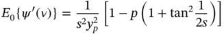
and more detail can be found in [124] and [121].
The advantage of this algorithm is that the error covariance ![]() for selected
for selected ![]() ‐point is always less than its value when the components of the transformed residual vector
‐point is always less than its value when the components of the transformed residual vector ![]() are independently and identically distributed with the least favorable marginal distribution [87]. As mentioned in [87], this worst‐case covariance is the optimum covariance for the case where the transformed residuals have this least favorable property. However, this estimate does not provide a saddle point for the MSE due to the constraints of the linear model, as is discussed in [124]. A similar problem was latter solved by Schick and Mitter in [160].
are independently and identically distributed with the least favorable marginal distribution [87]. As mentioned in [87], this worst‐case covariance is the optimum covariance for the case where the transformed residuals have this least favorable property. However, this estimate does not provide a saddle point for the MSE due to the constraints of the linear model, as is discussed in [124]. A similar problem was latter solved by Schick and Mitter in [160].
3.5.2 Robust Kalman Filter
An advanced approach to state estimation under uncertain matrices was developed by Khargonekar, Petersen, and Zhou in [89]. It was assumed that ![]() is coupled with the bounded uncertainty
is coupled with the bounded uncertainty ![]() as
as ![]() , where
, where ![]() and
and ![]() and
and ![]() are some known matrices. Then the error minimization problem is solved for the maximized norm‐bounded uncertain block. Based on this approach, many robust estimators have been developed for time‐varying and time‐invariant systems, assuming different operation conditions and environments [42,55,57,113,129,215]. Next we give a robust KF (RKF) scheme obtained by Xie, Soh, and de Souza in [215] and generalized in [111] for uncertain models with known uncorrelated white noise sources.
are some known matrices. Then the error minimization problem is solved for the maximized norm‐bounded uncertain block. Based on this approach, many robust estimators have been developed for time‐varying and time‐invariant systems, assuming different operation conditions and environments [42,55,57,113,129,215]. Next we give a robust KF (RKF) scheme obtained by Xie, Soh, and de Souza in [215] and generalized in [111] for uncertain models with known uncorrelated white noise sources.
Consider a discrete‐time state‐space model
and unite the uncertain matrices ![]() and
and ![]() in a parameter uncertainties vector as
in a parameter uncertainties vector as

where ![]() is an unknown uncertain matrix such that
is an unknown uncertain matrix such that ![]() for all
for all ![]() and
and ![]() ,
, ![]() , and
, and ![]() are known matrices of appropriate dimensions. Noise vectors
are known matrices of appropriate dimensions. Noise vectors ![]() and
and ![]() are supposed to be zero mean Gaussian and uncorrelated with the covariances
are supposed to be zero mean Gaussian and uncorrelated with the covariances ![]() and
and ![]() . It is also supposed that the system is quadratically stable.
. It is also supposed that the system is quadratically stable.
Quadratic stability of a linear system [142]: A system ((3.261)) is said to be quadratically stable if there exists a symmetric positive definite matrix
such that
(3.282)
for all admissible uncertainties
.
We can look for a stable KF estimate in the form of [215]
where ![]() and
and ![]() are to be determined in a way such that the estimation error
are to be determined in a way such that the estimation error ![]() is asymptotically stable and the
is asymptotically stable and the ![]() dynamics satisfies
dynamics satisfies
for a symmetric nonnegative definite matrix ![]() being an optimized upper bound of the error covariance to provide a guaranteed cost by solving the minimax problem
being an optimized upper bound of the error covariance to provide a guaranteed cost by solving the minimax problem
Now, since matrices ![]() and
and ![]() are specified, it is necessary to link the estimate (3.283) with the standard KF having no uncertainties.
are specified, it is necessary to link the estimate (3.283) with the standard KF having no uncertainties.
Because error ![]() depends on the system state, we can introduce an augmented vector
depends on the system state, we can introduce an augmented vector  and represent it recursively as
where  ,
,  ,
, ![]() , and
, and
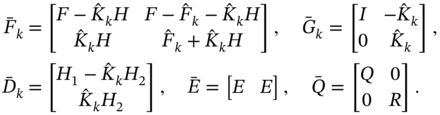
For given ![]() , the covariance matrix
, the covariance matrix ![]() of
of ![]() satisfies the following Lyapunov equation,
satisfies the following Lyapunov equation,
Since the uncertainty ![]() is unknown, we are interested in finding an upper bound
is unknown, we are interested in finding an upper bound ![]() of
of ![]() for all admissible
for all admissible ![]() . By replacing
. By replacing ![]() with
with ![]() , we arrive at the Lyapunov inequality
, we arrive at the Lyapunov inequality
and notice that ![]() holds for all
holds for all ![]() , provided that
, provided that ![]() for optimal estimates stays at a saddle.
for optimal estimates stays at a saddle.
It has been shown [111] that the filter (3.283) can be said to be robust if for some scaling factor ![]() there exists a bounded, positive definite, and symmetric
there exists a bounded, positive definite, and symmetric ![]() that satisfies the DDRE
that satisfies the DDRE
such that ![]() for
for  .
.
Without going into other details, which can be found in [215,233], we summarize the RKF estimate proposed in [111] with
where the necessary matrices with uncertain components are computed by

and the optimized covariance bound ![]() of the filtering error
of the filtering error ![]() is specified by solving the DDRE
is specified by solving the DDRE
subject to
over a horizon of ![]() data points in order for
data points in order for ![]() to be positive definite.
to be positive definite.
Let us now assume that the model in (3.289) and (3.290) has no uncertainties. By ![]() ,
, ![]() , and
, and ![]() , we thus have
, we thus have ![]() ,
, ![]() ,
, ![]() ,
, ![]() . Since the DDRE gives a recursion for the prior estimation error [185], we substitute
. Since the DDRE gives a recursion for the prior estimation error [185], we substitute ![]() , transform gain (3.273) to
, transform gain (3.273) to
where ![]() is the Kalman gain (3.79), and rewrite (3.292) as
is the Kalman gain (3.79), and rewrite (3.292) as

which also requires substituting ![]() with
with ![]() in (3.290) to obtain the prior estimate
in (3.290) to obtain the prior estimate
It now follows that the RKF (3.290)–(3.292) is the a priori RKF [111] and that without model uncertainties it reduces to the a priori KF (Algorithm 2). Note that the a posteriori RKF, which reduces to the a posteriori KF (Algorithm 1) without model uncertainties, can be found in [111].
3.5.3  Filtering
Although the ![]() approach was originally introduced and long after that has been under investigation in control theory [111],[34], its application to filtering has also attracted researchers owing to several useful features. Unlike KF, the
approach was originally introduced and long after that has been under investigation in control theory [111],[34], its application to filtering has also attracted researchers owing to several useful features. Unlike KF, the ![]() filter does not require any statistical information, while guaranteeing a prescribed level of noise reduction and robustness to model errors and temporary uncertainties.
filter does not require any statistical information, while guaranteeing a prescribed level of noise reduction and robustness to model errors and temporary uncertainties.
To present the ![]() filtering approach, we consider an LTI system represented in state space with equations
filtering approach, we consider an LTI system represented in state space with equations
where ![]() and
and ![]() are some error vectors, even deterministic, each with bounded energy. We wish to have a minimax estimator that for the maximized errors
are some error vectors, even deterministic, each with bounded energy. We wish to have a minimax estimator that for the maximized errors ![]() and
and ![]() minimizes the estimation error
minimizes the estimation error ![]() . Since the solution for Gaussian
. Since the solution for Gaussian ![]() and
and ![]() is KF, and arbitrary
is KF, and arbitrary ![]() and
and ![]() do not violate the estimator structure, the recursive estimate has the form
do not violate the estimator structure, the recursive estimate has the form
where the unknown gain ![]() is still to be determined.
is still to be determined.
The objective is to minimize ![]() in a way such that for the estimates obtained on a horizon
in a way such that for the estimates obtained on a horizon ![]() the following relation is satisfied
the following relation is satisfied

which leads to the following cost function of the a priori ![]() filter
filter

where ![]() is a positive definite matrix representing the uncertainty in the initial state, and the squared
is a positive definite matrix representing the uncertainty in the initial state, and the squared ![]() ‐norm
‐norm ![]() is depicted as
is depicted as ![]() or
or ![]() . Thus, the following minimax problem should be solved,
. Thus, the following minimax problem should be solved,
It was shown in [111] that for a cost (3.299) with ![]() there exists an a priori
there exists an a priori ![]() filter over the horizon
filter over the horizon ![]() if and only if there exists a positive definite solution
if and only if there exists a positive definite solution ![]() for
for ![]() to the following DDRE,
to the following DDRE,

where the filter gain is given by
![]() is the error matrix of
is the error matrix of ![]() , and
, and ![]() is the error matrix of
is the error matrix of ![]() . Note that
. Note that ![]() and
and ![]() have different meanings than the noise covariances
have different meanings than the noise covariances ![]() and
and ![]() in KF. It can be shown that when
in KF. It can be shown that when ![]() and
and ![]() are both zero mean Gaussian and uncorrelated with known covariances
are both zero mean Gaussian and uncorrelated with known covariances ![]() and
and ![]() , then substituting
, then substituting ![]() ,
, ![]() ,
, ![]() , and
, and ![]() , and neglecting the terms with large
, and neglecting the terms with large ![]() transform the a priori
transform the a priori ![]() filter to the a priori KF (Algorithm 2). Let us add that the a posteriori
filter to the a priori KF (Algorithm 2). Let us add that the a posteriori ![]() filter, which for Gaussian models becomes the a posteriori KF (Algorithm 1), is also available from [111].
filter, which for Gaussian models becomes the a posteriori KF (Algorithm 1), is also available from [111].
3.5.4 Game Theory  Filter
Another approach to ![]() filtering was developed using the game theory. An existence of the game‐theoretic solutions for minimax robust linear filters and predictors was examined by Martin and Mintz in [122]. Shortly thereafter, Verdú in [207] presented a generalization of Huber's approach to the minimax robust Bayesian statistical estimation problem of location with respect to the least favorable prior distributions. The minimax
filtering was developed using the game theory. An existence of the game‐theoretic solutions for minimax robust linear filters and predictors was examined by Martin and Mintz in [122]. Shortly thereafter, Verdú in [207] presented a generalization of Huber's approach to the minimax robust Bayesian statistical estimation problem of location with respect to the least favorable prior distributions. The minimax ![]() problem, solved on FH, considers the game cost function as a ratio of the filter error norm, which must be minimized, and the sum of the initial error norm and bounded error covariance norms, which must be maximized [14,163,190]. The corresponding recursive
problem, solved on FH, considers the game cost function as a ratio of the filter error norm, which must be minimized, and the sum of the initial error norm and bounded error covariance norms, which must be maximized [14,163,190]. The corresponding recursive ![]() filtering algorithm was obtained by Simon in [185], and it becomes KF without uncertainties.
filtering algorithm was obtained by Simon in [185], and it becomes KF without uncertainties.
In the standard formulation of game theory applied to model (3.278) and (3.279), the cost function for ![]() filtering is defined as follows:
filtering is defined as follows:

in order to find an estimate that minimizes ![]() . Similarly to the
. Similarly to the ![]() filter, (3.302) can be modified to
filter, (3.302) can be modified to

and the ![]() filtering estimate can be found by solving the minimax problem
filtering estimate can be found by solving the minimax problem
For the FE‐based model (3.296) and (3.297), the a priori game theory‐based ![]() filter derived in [185] using the cost (3.303) is represented with the following recursions
filter derived in [185] using the cost (3.303) is represented with the following recursions
where matrix ![]() is constrained by a positive definite matrix
is constrained by a positive definite matrix
It is the user choice to assign ![]() , which is introduced to weight the prior estimation error. If the goal is to weight all error components equally [115], one can set
, which is introduced to weight the prior estimation error. If the goal is to weight all error components equally [115], one can set ![]() . Because the cost
. Because the cost ![]() represents the squared norm error‐to‐error ratio and is guaranteed in the a priori
represents the squared norm error‐to‐error ratio and is guaranteed in the a priori ![]() filter to be
filter to be ![]() , the scalar bound
, the scalar bound ![]() must be small enough.
must be small enough.
To organize a posteriori filtering that matches the BE‐based model (3.32) and (3.33) with ![]() and
and ![]() , we can consider (3.286)–(3.288), replace
, we can consider (3.286)–(3.288), replace ![]() with
with ![]() and
and ![]() with
with ![]() , note that
, note that ![]() , refer to the derivation procedure given in (3.96), and arrive at the a posteriori
, refer to the derivation procedure given in (3.96), and arrive at the a posteriori ![]() filtering algorithm [180]
filtering algorithm [180]
which for given ![]() can be initiated with
can be initiated with ![]() .
.
For Gaussian noise and no disturbances, ![]() makes this filter an alternate KF (3.92)–(3.96). Otherwise, a properly set small
makes this filter an alternate KF (3.92)–(3.96). Otherwise, a properly set small ![]() improves the
improves the ![]() filter accuracy. It is worth noting that when
filter accuracy. It is worth noting that when ![]() approaches the boundary specified by the constraint, the
approaches the boundary specified by the constraint, the ![]() filter goes to instability. This means that in order to achieve the best possible effect,
filter goes to instability. This means that in order to achieve the best possible effect, ![]() must be carefully selected and its value optimized.
must be carefully selected and its value optimized.
3.6 Summary
As a process of filtering out erroneous data with measurement noise and simultaneously solving state‐space equations for unknown state variables at a given time instant, the state estimation theory is a powerful tool for many branches of engineering and science. To provide state estimation using computational resources, we need to know how to represent a dynamic process in the continuous‐time state space and then go correctly to the discrete‐time state space. Since a stochastic integral can be computed in various senses, the transition from continuous to discrete time is organized using either the FE method, associated with Itô calculus, or the BE method. The FE‐based state model predicts future state and is therefore fundamental in state feedback control. The BE‐based state model is used to solve various signal processing problems associated with filtering, smoothing, prediction, and identification.
The Bayesian approach is based on the use of Bayesian inference and is used to develop Bayesian estimators for linear and nonlinear state space models with noise having any distribution. For linear models, the Bayesian approach results in the optimal KF. Using the likelihood function, it is possible to obtain an ML estimator whose output converges to the Bayesian estimate as the number of measurement samples grows without bounds.
In the Gauss approach, the LS estimate is chosen so that the sum of the squares of the measurement residuals minimizes the mean square residual. The weighted LS approach considers the ML estimator as a particular case for Gaussian processes. The unbiased estimator only satisfies the unbiasedness condition and gives an estimate identical to LS.
The linear recursive KF algorithm can be a posteriori or a priori. The KF algorithm can be represented in various forms depending on the process, applications, and required outputs. However, the KF algorithm is poorly protected from initial errors, model errors, errors in noise statistics, and temporary uncertainties. The GKF is a modification of KF for time‐correlated and colored Gaussian noise. The KBF is an optimal state estimator in continuous time. For nonlinear state‐space models, the most widely used estimators are EKF, UKF, and PF.
Robust state estimation is required when the model is uncertain and/or operates under disturbances. The minimax approach is most popular when developing robust estimators. This implies minimizing estimation errors for a set of maximized uncertain parameters. Shown that a saddle‐point holds, the minimax estimator provides the worst‐case optimal performance and is therefore minimax robust.
3.7 Problems
- Find conditions under which the FE‐based and BE‐based state‐space models become identical. Which of these models provides the most accurate matched estimate?
- The FE‐based state space model is basic in feedback state control, and the BE‐based state space models is used for signal processing when prediction is not required. Why is this so? Give a reasonable explanation.
- Use the Bayes inference formula

and show that the ML estimate coincides with the most probable Bayesian estimate given a uniform prior distribution on the parameters.
- Consider the LS estimation problem of a constant quantity


where
 is the measurement residual,
  is a vector of multiple measurements of
  , and
, and  is a proper matrix. Derive the LS estimator of
  and relate it to the UFIR estimator.
 - Given an oscillatory system of the second order. Following Example 3.2, derive the matrix exponential for the system matrix
 , where
  is an angular bandwidth.
 - Solved problem: Matrix identity. Matrix
 is given by (3.92). Show that this matrix is identical to the error covariance matrix
  given by (3.79). Equate (3.92) and (3.79), substitute (3.78) and (3.77), and write

By the Woodbury matrix identity (A.7),

transform the previous relation as

Because
 ,
,  , and
, and  are symmetric, rearrange the matrix products as
introduce
 , rewrite as
  , substitute
  , provide the transformations, and end up with an identity
  , which proves that
  given by (3.92) and
  given by (3.79) are identical.
 - A linear discrete‐time state‐space model is augmented with the Gauss‐Markov CPN
 , where
  , and CMN
  , where
  . In what case is an estimator required to filter out only the CMN? What problem is solved by filtering out both CPN and CMN? Is there an application that only requires CPN filtering?
 - Solved problem: Steady state KF. Consider the KF Algorithm 1. Set
 and suppose that at a steady state
  and
and  . Then transform the a priori error covariance as

and arrive at the discrete algebraic Riccati equation (DARE)

Next, represent the Kalman gain as
 and end up with the steady state KF algorithm:
- The recursive LS estimate is given by

where matrix
 is computed recursively as
  . How does
  change with the increase in the number of measurement
  ? How is the recursive LS estimate related to UFIR estimate?
 - A constant quantity
 is measured in the presence of Laplace noise and is estimated using the median estimator

Modify this estimator under the assumption that
 is not constant and has
  states.
 - Under the Cauchy noise, a constant quantity
 is estimated using the myriad estimator [13]

where
 is the linearity parameter. Modify the myriad estimator for a dynamic quantity
  represented in state space by
  states.
 - Solved problem: Proof of ((3.222)). Consider the two‐filter smoother and its error covariance
 , substitute (3.220) and (3.221), and represent formally as
where
 and
and  are positive definite, symmetric, and invertible matrices. Using (A.10), write
  and transform the previous matrix equation to
that completes the proof of (3.222).
- The second‐order expansions of nonlinear functions are given by (3.228) and (3.229). Derive coefficients
 (3.232) and
  (3.233) using Hessian matrices (3.234) and (3.235). Find an explanation to the practical observation that the second‐order EKF either decreases or increases the estimation error, and nothing definite can be said about its performance.
 - The UKF has the following limitation: the same statistics can be predicted for different distributions. Suggest a feasible solution to improve performance using the high‐order statistics. Will it perform better than the second‐order EKF?
- The PF can dramatically improve estimation performance when the model has sever nonlinearity. Why is it impossible to fully guarantee the PF stability? What are the most effective ways to avoid the divergency in the PF? Why is there no guarantee that the PF will not diverge when the number of particles is insufficient?
- The robust KF approach for uncertain models suggests representing the uncertain system matrix
 and observation matrix
  using an unknown matrix
  as (3.281),

where
 and
and  are known and the newly introduced auxiliary matrices
  ,
,  , and
, and  are supposed to be known as well. Give examples when such a model is 1) advantageous, 2) can hardly be applied, and 3) is not feasible. Consider both the LTI and LTV systems.
 - In the presence of unknown norm‐bounded noise, the
 filtering estimate is given by (3.298) with the bias correction gain (3.301) and error covariance computed recursively by (3.300), where the optimal tuning factor
  guarantees the best filtering performance and robustness. How to specify
  ? Can we find
  analytically? What will happen if we set 1)
  and 2)
  ?
? - Solve the problems listed in the previous item, considering instead the tuning factor
 of the game theory
  filter, recursively represented by (3.307)–(3.310).
Notes
- 1 Carl Friedrich Gauss published his method of least squares in 1809 and claimed to have been in its possession since 1795. He showed that the arithmetic mean is the best estimate of the location parameter if the probability density is the (invented by him) normal distribution, now also known as Gaussian distribution.
- 2 Kalman derived his recursive filtering algorithm in 1960 by applying the Bayesian approach to linear processes with white Gaussian noise.
- 3 Notation
 means drawing
  samples
  ,
,  , from
  .
.