7
FIR Prediction and Receding Horizon Filtering
When the number of factors coming into play in a phenomenological complex is too large, scientific method in most cases fails. One need only think of the weather, in which case the prediction even for a few days ahead is impossible.
Albert Einstein, Science, Philosophy and Religion (1879–1955)
7.1 Introduction
A one‐step state predictive FIR approach called RH FIR filtering was developed for MPC. As an excerpt from [106] says, the term receding horizon was introduced “since the horizon recedes as time proceeds.” Therefore, it can be applied to any FIR structure and is thus redundant. But, with due respect to this still‐used technical jargon, we will keep it for one‐step FIR predictive filtering. Note that the theory of bias‐constrained (not optimal) RH FIR filtering was developed by W. H. Kwon and his followers [106].
The idea behind RH FIR filtering is to use an FE‐based model and derive an FIR predictive filter to obtain an estimate at ![]() over the horizon
over the horizon ![]() of most recent past observations. Since the predicted state can be used at the current discrete point, the properties of such filters are highly valued in digital state feedback control. Although an FIR filter that gives an estimate at
of most recent past observations. Since the predicted state can be used at the current discrete point, the properties of such filters are highly valued in digital state feedback control. Although an FIR filter that gives an estimate at ![]() over
over ![]() can also be used with this purpose by projecting the estimate to
can also be used with this purpose by projecting the estimate to ![]() , the RH FIR filter does it directly. Equivalently, the estimate obtained over
, the RH FIR filter does it directly. Equivalently, the estimate obtained over ![]() can be projected to
can be projected to ![]() using the one‐step FIR predictor.
using the one‐step FIR predictor.
In this chapter, we elucidate the modern theory of FIR prediction and RH FIR filtering. Some of the most interesting RH FIR solutions will also be considered, and we notice that the zero time step makes the RH FIR and FIR estimators equal in continuous time. Since the FIR predictor and the RH FIR filter can be transformed into each other by changing the time index, we will mainly focus on the FIR predictors due to their simpler forms.
7.2 Prediction Strategies
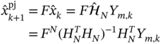
The current object state can most accurately be estimated at ![]() as
as ![]() using the a posteriori OFIR filter or KF. Since the estimate
using the a posteriori OFIR filter or KF. Since the estimate ![]() may be too biased for state feedback control at the next time index
may be too biased for state feedback control at the next time index ![]() , a one‐step predicted estimate
, a one‐step predicted estimate ![]() is required. There are two basic strategies for solving this problem (Fig. 7.1):
is required. There are two basic strategies for solving this problem (Fig. 7.1):
- Use the OFIR predictor and obtain the estimate
 over
over  as shown in Fig. 7.1a. This also implies that, by replacing
  with
with  , the estimate
  can be obtained over
  using the RH Kalman predictor (KP) [103] or RH FIR filtering.
 - Use the OFIR filter, obtain the a posteriori estimate
 , and then project it to
  as shown in Fig. 7.1b.
![Schematic illustration of two basic strategies to obtain the predicted estimate x˜k+1 at k+1 over [m,k]: (a) prediction and (b) projection from k to k+1.](https://imgdetail.ebookreading.net/2023/10/9781119863076/9781119863076__9781119863076__files__images__c07f001.png)
Figure 7.1 Two basic strategies to obtain the predicted estimate  at
at  over
over  : (a) prediction and (b) projection from
  to
to  .
.
Both these strategies are suitable for state feedback control but suffer from an intrinsic drawback: the predicted estimate is less accurate than the filtered one. Note that KP can be used here as a limited memory predictor (LMP) operating on ![]() to produce an estimate at
to produce an estimate at ![]() .
.
7.2.1 Kalman Predictor
The general form of the KP for LTV systems appears if we consider the discrete‐time state‐space model [100]
where ![]() ,
, ![]() ,
, ![]() ,
, ![]() ,
, ![]() ,
, ![]() ,
, ![]() ,
, ![]() , and
, and ![]() . The prior predicted estimate can be extracted from (7.1) as
. The prior predicted estimate can be extracted from (7.1) as
where ![]() is the predicted estimate at
is the predicted estimate at ![]() , and the measurement residual
, and the measurement residual ![]() gives the innovation covariance
gives the innovation covariance
Referring to (7.3), the prediction ![]() at
at ![]() can be written as
can be written as

and then, for the estimation error

the error covariance can be found to be
Further minimizing the trace of (7.7) by ![]() gives the optimal bias correction gain (KP gain)
gives the optimal bias correction gain (KP gain)
where the innovation covariance ![]() is given by (7.4). Using (7.8), the error covariance (7.7) can finally be written as
is given by (7.4). Using (7.8), the error covariance (7.7) can finally be written as
Thus, the estimates are updated in the KP algorithm for the given ![]() and
and ![]() as follows [103]:
as follows [103]:
and we notice that KP does not require the prior error covariance and operates only with ![]() . The KP can also work as an LMP on
. The KP can also work as an LMP on ![]() to obtain an estimate at
to obtain an estimate at ![]() for the given initial
for the given initial ![]() and
and ![]() at
at ![]() .
.
We can now start looking at FIR predictors, which traditionally require extended state and observation equations.
7.3 Extended Predictive State‐Space Model
Reasoning along similar lines as for the state‐space equations (4.1) and (4.2), introducing an extended predictive state vector
and taking other extended vectors from (4.4)–(4.6), (4.12), and (4.13), we extend the model (7.1) and (7.2) as
where the extended matrices are given as ![]() ,
,

matrix ![]() has the same structure and components as
has the same structure and components as ![]() if we substitute
if we substitute ![]() with
with ![]() ,
, ![]() is given by (4.9),
is given by (4.9), ![]() becomes
becomes ![]() if we substitute
if we substitute ![]() with
with ![]() , and matrix
, and matrix ![]() is diagonal. Hereinafter, the superscript “
is diagonal. Hereinafter, the superscript “![]() ” is used to denote matrices in prediction models.
” is used to denote matrices in prediction models.
As with the FE‐based model, extended equations 7.14 and (7.15) will be used to derive FIR predictors and RH FIR filters.
7.4 UFIR Predictor
The UFIR predictor can be derived if we define the prediction as
and extract from (7.14) the model
where ![]() is the last row vector in
is the last row vector in ![]() and so is
and so is ![]() in
in ![]() .
.
The unbiasedness condition ![]() applied to (7.20) and (7.21) gives two unbiasedness constraints
applied to (7.20) and (7.21) gives two unbiasedness constraints
which have the same forms as (4.21) and (4.22) previously found for the OFIR filter, but with modified matrices and gains ![]() and
and ![]() .
.
7.4.1 Batch UFIR Predictor
In batch form, the UFIR predictor appears by solving (7.22) for the fundamental gain ![]() , which gives
, which gives
where ![]() is the auxiliary block matrix and the GNPG matrix
is the auxiliary block matrix and the GNPG matrix ![]() is square and symmetric. Using (7.23), the UFIR predicted estimate can be written in the batch form as
is square and symmetric. Using (7.23), the UFIR predicted estimate can be written in the batch form as
where the gain ![]() is defined by (7.24b). The error covariance is given by
is defined by (7.24b). The error covariance is given by
where the system and observation error residual matrices are defined as
Again we notice that the form (7.26) is unique for all bias‐constrained FIR state estimators, where the individual properties are collected in the error residual matrices, such as (7.27) and (7.28).
7.4.2 Iterative Algorithm using Recursions
Recursions for the batch UFIR prediction (7.25) can be found similarly to the batch UFIR filtering estimate if we represent ![]() as the sum of the homogeneous estimate
as the sum of the homogeneous estimate ![]() and the forced estimates
and the forced estimates ![]() . To do this, we will use the following matrix decompositions,
. To do this, we will use the following matrix decompositions,

To find a recursion for ![]() using
using ![]() taking from (7.29), we transform the inverse of GNPG
taking from (7.29), we transform the inverse of GNPG ![]() as
as

This gives the following direct and inverse recursive forms,
Likewise, we represent the product ![]() as
as
and then transform the homogeneous estimate ![]() to
to
where the GNPG ![]() is computed recursively using (7.30).
is computed recursively using (7.30).
To find a recursive form for the forced estimate in (7.25), it is necessary to find recursions for the two components in (7.25) separately. To this end, we refer to (7.29) and first obtain
Next, we use ![]() , take some decompositions from (7.29), and transform the remaining component
, take some decompositions from (7.29), and transform the remaining component ![]() as
as
Combining (7.34) and (7.35), we finally write the forced estimate in the form
The UFIR prediction ![]() can now be represented with the recursion
can now be represented with the recursion
and the pseudocode of the iterative UFIR prediction algorithm can be listed as Algorithm 17. This algorithm iteratively updates the estimates on ![]() , starting with estimates
, starting with estimates ![]() and
and ![]() computed over
computed over ![]() in short batch forms, and the final prediction appears at
in short batch forms, and the final prediction appears at ![]() .
.
Now, let us again note two forms of UFIR state estimators suitable for stochastic state feedback control. One can replace ![]() by
by ![]() in (7.37) and consider
in (7.37) and consider ![]() as an RH UFIR filtering estimate. Otherwise, the same task can be accomplished by taking the UFIR filtering estimate at
as an RH UFIR filtering estimate. Otherwise, the same task can be accomplished by taking the UFIR filtering estimate at ![]() and projecting it onto
and projecting it onto ![]() using the system matrix
using the system matrix ![]() . While these solutions are not completely equivalent, they provide a similar control quality because both are unbiased.
. While these solutions are not completely equivalent, they provide a similar control quality because both are unbiased.
Equivalence of Projected and Predicted Estimates
So far, we have looked at LTV systems, for which the BE‐ and FE‐based state models cannot be converted into each other, and the projected and predicted UFIR estimates are not equivalent. However, in the special case of the LTI system without input, the equivalence of such structures can be shown.
Consider (6.10a), assume that all matrices are time‐invariant, substitute the subscript ![]() in matrices with
in matrices with ![]() , and write
, and write
where ![]() is the UFIR filter gain. Then the projected estimate
is the UFIR filter gain. Then the projected estimate ![]() can be written as
can be written as
and the predicted estimate ![]() can be written as
can be written as
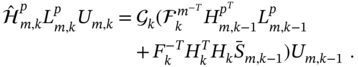
It is easy to show now that for LTI systems the matrices ![]() and
and ![]() are identical and thus the predicted and projected UFIR estimates are equivalent,
are identical and thus the predicted and projected UFIR estimates are equivalent, ![]() . It also follows that, for LTI systems without input, the UFIR prediction can be organized using the projected estimate as
. It also follows that, for LTI systems without input, the UFIR prediction can be organized using the projected estimate as ![]() .
.
UFIR prediction: For LTI systems, the UFIR predicted estimate
and projected estimate
are equivalent.
This statement was confirmed by Example 7.1, where it was numerically demonstrated that the predicted and projected UFIR estimates are identical.
7.4.3 Recursive Error Covariance
There are two ways to find recursive forms for the error covariance of the UFIR predictor. We can start with (7.25), find recursions for each of the batch components, and then combine them in the final form. Otherwise, we can obtain ![]() using recursion (7.37). To make sure that these approaches lead to the same results, next we give the most complex derivation and postpone the simplest to “Problems.”
using recursion (7.37). To make sure that these approaches lead to the same results, next we give the most complex derivation and postpone the simplest to “Problems.”
Consider the batch error covariance (7.26) and represent it as
where the matrices are: ![]() ,
, ![]() ,
, ![]() ,
, ![]() , and
, and ![]() .
.
Following the derivation procedure applied in Chapter to the error covariance of the UFIR filter, we represent components of (7.38) as
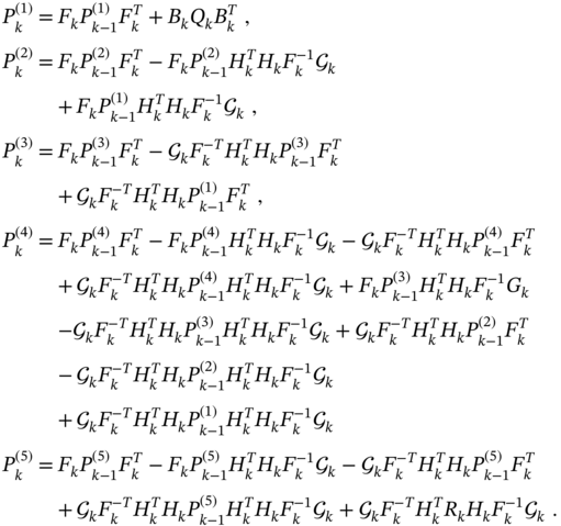
Combining these matrices in (7.38), we obtain the following recursive form for the error covariance,

All that follows from (7.39) is that it is unified by the KP error covariance (7.7) if we introduce the bias correction gain ![]() instead of the Kalman gain. It should also be noted that recursion (7.39) can be obtained much easier if we start with the recursive estimate (7.37). The corresponding derivation is postponed to “Problems.”
instead of the Kalman gain. It should also be noted that recursion (7.39) can be obtained much easier if we start with the recursive estimate (7.37). The corresponding derivation is postponed to “Problems.”
7.5 Optimal FIR Predictor
In the discrete convolution‐based batch form, the OFIR predictive estimate can be defined similarly to the OFIR filtering estimate as
where the gains ![]() and
and ![]() are to be found by minimizing the MSE with respect to the model
are to be found by minimizing the MSE with respect to the model
which is given by the last row vector in (7.14) and where ![]() is the last row vector in
is the last row vector in ![]() and so is
and so is ![]() in
in ![]() .
.
7.5.1 Batch Estimate and Error Covariance
For the estimation error ![]() , determined taking into account (7.40) and (7.41), we apply the orthogonality condition as
, determined taking into account (7.40) and (7.41), we apply the orthogonality condition as
and transform it to

where the error residual matrices given by
ensure optimal cancellation of regular (bias) and random errors at the OFIR predictor output.
For zero input, ![]() , relation (7.43) gives the fundamental gain
, relation (7.43) gives the fundamental gain ![]() for the OFIR predictor,
for the OFIR predictor,
where ![]() ,
, ![]() ,
, ![]() , and the UFIR predictor gain
, and the UFIR predictor gain ![]() is given by (7.24b).
is given by (7.24b).
Since the forced impulse response ![]() is determined by constraint (7.23), the batch OFIR predictor (7.40) eventually becomes
is determined by constraint (7.23), the batch OFIR predictor (7.40) eventually becomes
where ![]() and
and ![]() are real vectors containing data collected on
are real vectors containing data collected on ![]() . It can be seen that, for deterministic models with zero noise, we have
. It can be seen that, for deterministic models with zero noise, we have ![]() , and thus the OFIR predictor becomes the UFIR predictor.
, and thus the OFIR predictor becomes the UFIR predictor.
The batch error covariance ![]() for the OFIR predictor is given by
for the OFIR predictor is given by

where the error residual matrices are provided with (7.44)–(7.46). Next, we will find recursive forms required to develop an iterative OFIR predictive algorithm based on (7.49).
7.5.2 Recursive Forms and Iterative Algorithm
Using expansions (7.29), the recursions for the OFIR predictor can be found similarly to the OFIR filter, as stated in the following theorem.
A simple glance at the result reveals that the iterative OFIR prediction algorithm (theorem 7.1), operating on ![]() , employs the KP recursions given by (7.10)–(7.13). We wish to note this property as fundamental, since all estimators that minimize MSE in the same linear stochastic model can be transformed into each other. It also follows, as an extension, that (7.48) represents the batch KP by setting the starting point to zero,
, employs the KP recursions given by (7.10)–(7.13). We wish to note this property as fundamental, since all estimators that minimize MSE in the same linear stochastic model can be transformed into each other. It also follows, as an extension, that (7.48) represents the batch KP by setting the starting point to zero, ![]() .
.
It is also worth mentioning that the OFIR projector and predictor give almost identical estimates (Example 7.2). Thus, it follows that a simple projection of the state from ![]() to
to ![]() through the system matrix can effectively serve not only for unbiased prediction but also for suboptimal prediction.
through the system matrix can effectively serve not only for unbiased prediction but also for suboptimal prediction.
7.6 Receding Horizon FIR Filtering
Suboptimal RH FIR filters subject to the unbiasedness constraint were originally obtained for stationary stochastic processes in [105] and for nonstationary stochastic processes in [106]. Both solutions were called the minimum variance FIR (MVF) filter. Therefore, to distinguish the difference, we will refer to them as the MVF‐I filter and the MVF‐II filter, respectively. Note that MVF filters turned out to be the first practical solutions in the family of FIR state estimators, although their derivation draws heavily on the early work [97]. Next, we will derive both MVF filters, keeping the original ideas and derivation procedures, but accepting the definitions given in this book.
7.6.1 MVF‐I Filter for Stationary Processes
The MVF‐I filter resembles the OUFIR predictive filter but ignores the process dynamics and thus has most in common with the weighted LS estimate (3.61), which is suitable for stationary processes.
To obtain the MVF‐I solution, let us start with the model in (7.1) and (7.2). Since the MVF‐I filter ignores the process dynamics, it only needs the observation equation, which can be extended on the horizon ![]() as
as
where the following extended vectors were introduced,
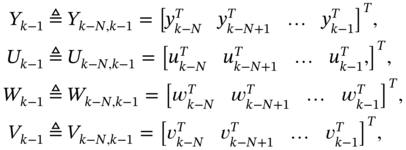
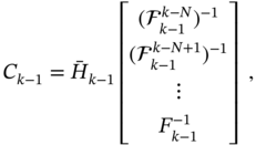
and the extended matrices ![]() ,
, ![]() ,
, ![]() , and
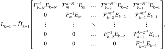
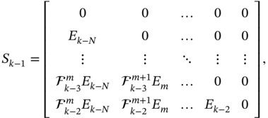
, and ![]() are defined as
are defined as
Note that matrix ![]() becomes equal to matrix
becomes equal to matrix ![]() if we replace
if we replace ![]() by
by ![]() .
.
We can now define the RH FIR filtering estimate as

provide the averaging of both sides of (7.71), and obtain two unbiasedness constraints,
Now, substituting (7.72) and (7.73) into (7.71) gives
the estimation error becomes
and the error covariance ![]() can be written as
can be written as
where ![]() and
and ![]() are the error residual matrices.
are the error residual matrices.
To find the gain ![]() subject to constraint (7.72), the trace of
subject to constraint (7.72), the trace of ![]() can be minimized with
can be minimized with ![]() using the Lagrange multiplier method as
using the Lagrange multiplier method as

that, if we introduce ![]() , gives
, gives

Multiplying both sides of (7.75) by the nonzero ![]() from the left‐hand side and using (7.72), we obtain the Lagrange multiplier as
from the left‐hand side and using (7.72), we obtain the Lagrange multiplier as

and then the substitution of ![]() in (7.75) gives the gain [105]
in (7.75) gives the gain [105]
We finally represent the MVF‐I filter (7.70) with
and notice that the error covariance for (7.77b) is defined by (7.74b).
It can be seen that the MVF‐I filter has the form of the ML‐I FIR filter (4.98a) and thus belongs to the family of ML state estimators. The difference is that the error residual matrix ![]() in (7.74b) does not include the matrix
in (7.74b) does not include the matrix ![]() containing information of the process dynamics. Therefore, the MVF‐I filter is most suitable for stationary and quasistationary processes. For LTI systems, recursive computation of (7.77b) is provided in [105,106]. In the general case of LTV systems, recursions can be found using the OUFIR‐II filter derivation procedure, and we postpone it to “Problems.”
containing information of the process dynamics. Therefore, the MVF‐I filter is most suitable for stationary and quasistationary processes. For LTI systems, recursive computation of (7.77b) is provided in [105,106]. In the general case of LTV systems, recursions can be found using the OUFIR‐II filter derivation procedure, and we postpone it to “Problems.”
7.6.2 MVF‐II Filter for Nonstationary Processes
A more general MVF‐II filter was derived in [106] using a similar procedure as for the OUFIR‐II filter. However, to obtain an estimate at ![]() , the MVF‐II filter takes data from
, the MVF‐II filter takes data from ![]() , while the OUFIR‐II filter from
, while the OUFIR‐II filter from ![]() .
.
The MVF‐II filter can be obtained using the model in (7.14) and (7.15), if we keep the definitions for MVF‐I, introduce a time shift, and write
where the extended matrices are given by
matrix ![]() is equal to matrix
is equal to matrix ![]() by replacing
by replacing ![]() with
with ![]() ,
, ![]() is the last row vector in
is the last row vector in ![]() and so is
and so is ![]() in
in ![]() , and matrix
, and matrix ![]() is diagonal.
is diagonal.
We can now define the MVF‐II estimate and transform using (7.79) as

Introducing ![]() and applying the unbiasedness conditions to (7.85) and (7.78), we next obtain the unbiasedness constraints
and applying the unbiasedness conditions to (7.85) and (7.78), we next obtain the unbiasedness constraints
define the estimation error as ![]() , use the constraints (7.86) and (7.87), transform
, use the constraints (7.86) and (7.87), transform ![]() to
to
and find the error covariance
To embed the unbiasedness, we solve the optimization problem
by putting to zero the derivatives of the trace of the matrix function with respect to ![]() and
and ![]() , and obtain
, and obtain
Then multiplying both sides of (7.91) from the left‐hand side with ![]() and using (7.86) gives the Lagrange multiplier
and using (7.86) gives the Lagrange multiplier
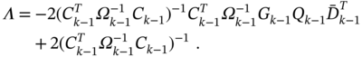
We finally substitute (7.92) into (7.91), find the gain ![]() in the form
in the form

represent the MVF‐II filtering estimate (7.84) as
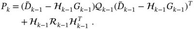
where ![]() is given by (7.93), and write the error covariance (7.89) in the standard form
is given by (7.93), and write the error covariance (7.89) in the standard form
where the error residual matrices are defined by
It can now be shown that for LTI systems the gain (7.93) is equivalent to the gain (4.69a) of the OUFIR‐II filter. Since the OUFIR‐II gain is identical to the ML‐I FIR gain (4.113b), it follows that the MVF‐II filter also belongs to the class of ML estimators. Therefore, the recursions for the MVF‐II filter can be taken from Algorithm 8, not forgetting that this algorithm has the following disadvantages: 1) exact initial values are required to initialize iterations, 2) it is less accurate than the OFIR algorithm, and 3) it is more complex than the OFIR algorithm. All of this means that optimal unbiased recursions persisting for an MVF‐II filter will have limited advantages over Kalman recursions. Finally, the recursive forms found in [106] for the MVF‐II filter are much more complex than those in Algorithm 8.
7.7 Maximum Likelihood FIR Predictor
Like the standard ML FIR filter, the ML FIR predictor has two possible algorithmic implementations. We can obtain the ML FIR prediction at ![]() on the horizon
on the horizon ![]() in what we will call the ML‐I FIR predictor. We can also first obtain the ML FIR backward estimate at the start point
in what we will call the ML‐I FIR predictor. We can also first obtain the ML FIR backward estimate at the start point ![]() over
over ![]() and then project it unbiasedly onto
and then project it unbiasedly onto ![]() in what we will call the ML‐II FIR predictor. Because the ML approach is unbiased, the unbiased projection in the ML‐II FIR predictor is justified for practical purposes.
in what we will call the ML‐II FIR predictor. Because the ML approach is unbiased, the unbiased projection in the ML‐II FIR predictor is justified for practical purposes.
7.7.1 ML‐I FIR Predictor
To derive the ML‐I FIR predictor, we consider the state‐space model
extend it as (7.14) and (7.15), extract ![]() , and obtain
, and obtain
The ML‐I FIR predicted estimate can now be determined for data taken from ![]() by maximizing the likelihood
by maximizing the likelihood ![]() of
of ![]() as
as
The solution to the maximization problem (7.102) can be found if we extract ![]() from (7.100) as
from (7.100) as ![]() , substitute into (7.101), and then represent (7.101) as
, substitute into (7.101), and then represent (7.101) as
where ![]() and all random components are combined in
and all random components are combined in
For a multivariate normal distribution, the likelihood of ![]() is given by
is given by
where the covariance matrix is defined as
The maximization problem (7.102) can now be equivalently replaced by the minimization problem
which assumes minimization of the quadratic form. Referring to (7.106b), we find a solution to (7.107) in the form
and write the error covariance using (7.104) as
What finally comes is that the prediction (7.108) differs from the previously obtained ML‐I FIR filtering estimate (4.98a) only in the modified matrices ![]() and
and ![]() , which reflect the features of the state model (7.98) and the predictive estimate (7.102).
, which reflect the features of the state model (7.98) and the predictive estimate (7.102).
7.7.2 ML‐II FIR Predictor
As mentioned earlier, the ML‐II FIR prediction appears if we first estimate the initial state at ![]() over
over ![]() and then project it forward to
and then project it forward to ![]() . The first part of this procedure has already been supported by (4.114)–(4.119). Applied to the model in (7.98) and (7.99), this gives the a posteriori ML FIR estimate
. The first part of this procedure has already been supported by (4.114)–(4.119). Applied to the model in (7.98) and (7.99), this gives the a posteriori ML FIR estimate
In turn, the unbiased projection of (7.110) onto ![]() can be obtained as
can be obtained as

to be an ML‐II FIR predictive estimate, the error covariance of which is given by
It is now easy to show that the ML‐II FIR predictor (7.111) has the same structure of the error covariance (7.112) as the structure (7.74b) of the MVF‐I filter (7.77b), and we conclude that these estimates can be converted to each other by introducing a time shift.
7.8 Extended OFIR Prediction
When state feedback control is required for nonlinear systems, then linear estimators generally cannot serve, and extended predictive filtering or prediction is used. To develop an EOFIR predictor, we assume that the process and its observation are both nonlinear and represent them with the following state and observation equations
Now the EOFIR predictor can be obtained similarly to the EOFIR filter if we expand the nonlinear functions with the Taylor series. Assuming that the functions ![]() and
and ![]() are sufficiently smooth, we expand them around the available estimate
are sufficiently smooth, we expand them around the available estimate ![]() using the second‐order Taylor series as
using the second‐order Taylor series as
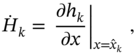
where the increment ![]() is equivalent to the estimation error, the Jacobian matrices are given by
is equivalent to the estimation error, the Jacobian matrices are given by

the second‐order terms are determined as [15]
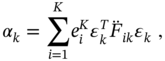

and the Hessian matrices are defined by

where ![]() ,
, ![]() , and
, and ![]() ,
, ![]() , are the
, are the ![]() th and
th and ![]() th components of
th components of ![]() and
and ![]() , respectively. Also,
, respectively. Also, ![]() and
and ![]() are Cartesian basis vectors with ones in the
are Cartesian basis vectors with ones in the ![]() th and
th and ![]() th components and zeros elsewhere.
th components and zeros elsewhere.
The nonlinear model in (7.113) and (7.114) can thus be linearized as
where ![]() is the modified observation, in which
is the modified observation, in which
is a correction vector, and ![]() given by
given by
plays the role of an input signal.
It follows from this model that the second‐order additions ![]() and
and ![]() affect only
affect only ![]() and
and ![]() . If
. If ![]() and
and ![]() have little effect on the prediction, they can be omitted as in the EOFIR‐1 predictor. Otherwise, one should use the EOFIR‐II predictor.
have little effect on the prediction, they can be omitted as in the EOFIR‐1 predictor. Otherwise, one should use the EOFIR‐II predictor.
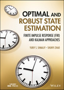
The pseudocode of the EOFIR prediction algorithm serving both options is listed as Algorithm 18, where the matrix ![]() is computed by (7.125) using the Taylor series expansions. It can be seen that the nonlinear functions
is computed by (7.125) using the Taylor series expansions. It can be seen that the nonlinear functions ![]() and
and ![]() are only used here to update the prediction, while the error covariance matrix is updated using the extended matrices. Another feature is that Algorithm 18 is universal for both EOFIR‐I and EOFIR‐II predictors. Indeed, in the case of the EOFIR‐I predictor, the terms
are only used here to update the prediction, while the error covariance matrix is updated using the extended matrices. Another feature is that Algorithm 18 is universal for both EOFIR‐I and EOFIR‐II predictors. Indeed, in the case of the EOFIR‐I predictor, the terms ![]() and
and ![]() vanish in the matrix
vanish in the matrix ![]() , and for the EOFIR‐II predictor they must be preserved. It should also be noted that the more sophisticated second‐order EOFIR‐II predictor does not demonstrate clear advantages over the EOFIR‐I predictor, although we have already noted this earlier.
, and for the EOFIR‐II predictor they must be preserved. It should also be noted that the more sophisticated second‐order EOFIR‐II predictor does not demonstrate clear advantages over the EOFIR‐I predictor, although we have already noted this earlier.
7.9 Summary
Digital stochastic control requires predictive estimation to provide effective state feedback control, since filtering estimates may be too biased at the next time point. Prediction or predictive filtering can be organized using any of the available state estimation techniques. The requirement for such structure is that they must provide one‐step prediction with maximum accuracy. This allows for suboptimal state feedback control, even though the predicted estimate is less accurate than the filtering estimate. Next we summarize the most important properties of the FIR predictors and RH FIR filters.
To organize one‐step prediction at ![]() , the RH FIR predictive filter can be used to obtain an estimate over the data FH
, the RH FIR predictive filter can be used to obtain an estimate over the data FH ![]() . Alternatively, we can use any type of FIR predictor to obtain an estimate at
. Alternatively, we can use any type of FIR predictor to obtain an estimate at ![]() over
over ![]() . If necessary, we can change the time variable to obtain an estimate at
. If necessary, we can change the time variable to obtain an estimate at ![]() over
over ![]() . We can also use the FIR filtering estimate available at
. We can also use the FIR filtering estimate available at ![]() and project it to
and project it to ![]() using the system matrix.
using the system matrix.
The iterative OFIR predictor uses the KP recursions. The difference between the OFIR predictor and OFIR filter estimates is poorly discernible when these structures fully fit the model. But in the presence of uncertainties, the predictor can be much less accurate than the filter. For LTI systems without input, the UFIR prediction is equivalent to a one‐step projected UFIR filtering estimate. The UFIR and OFIR predictors can be obtained in batch form and in an iterative form using recursions.
The MVF‐I filter and the ML‐II FIR predictor have the same batch form, and both these estimators belong to the family of ML state estimators. The MVF‐I filter is suitable for stationary and quasistationary stochastic processes, while the MVF‐II filter is suitable for nonstationary stochastic processes. The EOFIR predictor can be obtained similarly to the extended OFIR filter using first‐ or second‐order Taylor series expansions.
7.10 Problems
- Following the derivation of the KP algorithm (7.10)–(7.13), obtain the LMP algorithm at
 over
over  and at
  over
over  .
. - Given the state‐space model in (7.1) and (7.2), using the Bayesian approach, derive the KP and show its equivalence to the algorithm (7.10)–(7.13).
- The risk function of the RH FIR estimate
 is given by
Show that the inequality
 holds if
  satisfies the cost function
 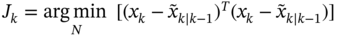 .
. - A system is represented in state space with the following equations:
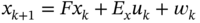 and
and  . Extend this model on
  and derive the UFIR predictor.
 - Consider the system described in item 4 and derive the OFIR predictor.
- Given the following harmonic two‐state space model
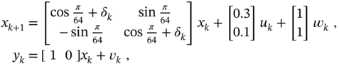
where
 and
and  are white Gaussian with the covariances
  and
and  and the disturbance
  is induced from 350 to 400, simulate this process for the initial state
  and estimate
  numerically using different FIR predictors. Select the most and less accurate predictors among the predictors OFIR, UFIR, ML‐I FIR, and ML‐II FIR.
 - Consider the problem described in item 6, estimate
 using the MVF‐I and MVF‐II predictive filters, and compare the errors. Explain the difference between the predictive estimates.
 - The error covariances
 and
and  of two FIR predictors are given by the solutions of the following DDREs

Find the difference
 and analyze the dependence of
  on the system noise covariances
  and
and  .
. - Consider the error residual matrices
 and
and  of the UFIR predictor (7.25) and explain why a decrease in GNPG
  improves measurement noise reduction.
 - Explain why an FIR filter and an FIR predictor that satisfy the same cost function are equivalent in continuous time.
- Given the state‐space model,
 and
and  , and the KP and KF estimates, respectively,
(7.127)
, and the KP and KF estimates, respectively,
(7.127)
under what conditions do these estimates 1) become equivalent and 2) cannot be converted into each other?
- Given the MVF‐I filter (7.77b), following the derivation of the OUFIR‐II filter, find recursive forms for the MVF‐I filter and design an iterative algorithm.
- The recursive form for the batch error covariance (7.26), which corresponds to the batch UFIR predictor (7.25), is given by (7.39) as

Obtain this recursion using the recursive UFIR predictor estimate

- The MVF‐II filter is represented by the fundamental gain (7.93). Referring to the similarity with the OUFIR filter, find recursive forms and design an iterative algorithm for the MVF‐II filter.
- Consider the state‐space model
 and
and  . Define the MVF predictive filtering estimate as
and obtain the gains
 and
and  for
for  .
. - The state of the LTI system without input is estimated using OFIR filtering as
 (4.30b). Project this estimate to
  as
as  . Also consider the OFIR predicted estimate
  . Under what conditions do the projected and predicted estimates 1) become identical and 2) cannot be converted into one another?
 - The batch UFIR prediction is given by

Compare this prediction with the LS prediction and highlight the differences.
- A nonlinear system is represented in state space with the equations
 and
and  . Suppose that the white Gaussian noise vectors
  and
and  have low intensity components and that the input
  is known. Apply the first‐order Taylor series expansion and obtain an EOFIR predictor.
 - Consider the previously described problem, apply the same conditions, and obtain a first‐order EFIR predictor and an RH EFIR filter.
- The gain of the RH MVF filter is specified by (7.76) as

Can this gain be applied when the system matrix
 is singular? If not, modify this gain to be applicable for a singular matrix
  .
. - A wireless network is represented with the following state‐space model,

where
 is the observation provided by
  sensors and
  . Zero mean mutually uncorrelated white Gaussian noise vectors
  and
and  have the covariances
  and
and  , respectively. Think about how to obtain a UFIR predictor and an RH UFIR filter with some kind of consensus in measurements to simplify the algorithm.