11
Applications of FIR State Estimators
Design is not how it looks like and feels like. Design is how it works.
Steve Jobs (Apple Inc. cofounder and former CEO)
This chapter is the last, and it is now a proper place to give examples of practical applications of FIR state estimators. As the approach suggests, many useful FIR engineering algorithms can be developed to solve filtering, smoothing, and prediction problems on data finite horizons under diverse operation conditions in different environments. For Gaussian processes, the batch OFIR state estimator has proven to be the most accurate in the MSE sense, and the supporting recursive KF algorithm and its various modifications have found a huge number of applications. The OUFIR state estimator and RH MVF are commonly used in the canonical ML FIR batch form, since the recursive forms for these batches are more complex than Kalman recursions. The UFIR state estimator is blind on optimal horizons (has no other tuning factors) and is thus robust, unlike the OFIR and OUFIR estimators. Therefore, the iterative UFIR filtering algorithm using recursions has found practical applications as an alternative to KF in uncertain environments. It is worth noting that there has been no further development of the original LMF idea, because LMF is nothing more than KF operating on data finite horizons. In recent decades, there has appeared a big class of norm‐bounded ![]() ,
, ![]() ,
, ![]() ‐to‐
‐to‐![]() ,
, ![]() , and hybrid FIR state estimators. Such estimators are called robust, but their development for practical use has been carried out to a much lesser extent and awaits further development.
, and hybrid FIR state estimators. Such estimators are called robust, but their development for practical use has been carried out to a much lesser extent and awaits further development.
In this chapter, we provide examples of practical applications of FIR state estimators in various fields and different environments using batch and iterative algorithms.
11.1 UFIR Filtering and Prediction of Clock States
The IEEE Standard 1139‐2008 [75] and International Telecommunication Union (ITU‐T) recommendation G.810 [77] suggest that a clock has three states, namely, the time interval error (TIE), fractional frequency offset, and linear frequency drift rate. The problem with accurate estimation of clock state has a lot to do with the clock oscillator noise, which has a slow flicker (technical) Gaussian component having the PSD slope ![]() in the Fourier frequency
in the Fourier frequency ![]() domain. Even modified for CPN [182], which has the PSD slope
domain. Even modified for CPN [182], which has the PSD slope ![]() , the KF is unable to track accurately the
, the KF is unable to track accurately the ![]() behaviors. In GPS‐based timekeeping using one pulse per second (1PPS) signals, the problem is complicated with the uniformly distributed (non‐Gaussian) measurement noise and GPS time uncertainties caused by different satellites in a view. Therefore, the UFIR filter, which ignores zero mean noise, better fulfils the requirement of the IEEE Standard 1139‐2008 [75] that “an efficient and unbiased estimator is preferred” for clock applications [166].
behaviors. In GPS‐based timekeeping using one pulse per second (1PPS) signals, the problem is complicated with the uniformly distributed (non‐Gaussian) measurement noise and GPS time uncertainties caused by different satellites in a view. Therefore, the UFIR filter, which ignores zero mean noise, better fulfils the requirement of the IEEE Standard 1139‐2008 [75] that “an efficient and unbiased estimator is preferred” for clock applications [166].
11.1.1 Clock Model
In accordance with [75] and [77], the clock TIE ![]() caused by oscillator instabilities is modeled in continuous time
caused by oscillator instabilities is modeled in continuous time ![]() with the finite Taylor series as
with the finite Taylor series as
where ![]() is the initial TIE (first state) at
is the initial TIE (first state) at ![]() ,
, ![]() is the initial fractional frequency offset (second state), and
is the initial fractional frequency offset (second state), and ![]() is the initial linear frequency drift rate (third state). Noise
is the initial linear frequency drift rate (third state). Noise ![]() is completely defined by the clock oscillator random phase deviation component
is completely defined by the clock oscillator random phase deviation component ![]() and nominal frequency
and nominal frequency ![]() in Hz. The IEEE standard [75] states that
in Hz. The IEEE standard [75] states that ![]() is affected by different kinds of independent phase and frequency fluctuations (white, flicker, and random walks), which PSD slopes can be measured in the Fourier frequency domain.
is affected by different kinds of independent phase and frequency fluctuations (white, flicker, and random walks), which PSD slopes can be measured in the Fourier frequency domain.
In state space, (11.1) is represented with the SDE
in which ![]() is the clock state vector and
is the clock state vector and ![]() is the zero mean Gaussian noise vector having the covariance
is the zero mean Gaussian noise vector having the covariance ![]() . In this vector,
. In this vector, ![]() is the frequency noise,
is the frequency noise, ![]() is the linear frequency drift noise, and
is the linear frequency drift noise, and ![]() is noise in the first time derivative of the linear frequency drift. Note that
is noise in the first time derivative of the linear frequency drift. Note that ![]() is nonstationary on a long time scale, although it is typically assumed to be stationary on a short time. The clock state transition matrix
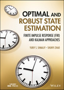
is nonstationary on a long time scale, although it is typically assumed to be stationary on a short time. The clock state transition matrix ![]() is specified by
is specified by

In discrete time index ![]() , model (11.2) is represented with
, model (11.2) is represented with
where the clock matrix ![]() is defined by the matrix exponential
is defined by the matrix exponential ![]() to be
to be
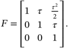
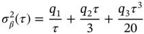
The zero mean Gaussian noise vector ![]() and its covariance
and its covariance ![]() are defined by, respectively,
are defined by, respectively,


and we notice that (11.6) and (11.7) can be applied to all kinds of phase and frequency noise sources.
In timekeeping, only the first clock state (TIE) is commonly measured. Therefore, the observation equation becomes
where ![]() , and
, and ![]() is zero mean noise, which is not Gaussian in the 1PPS output of a GPS timing receiver.
is zero mean noise, which is not Gaussian in the 1PPS output of a GPS timing receiver.
11.1.2 Clock State Estimation Over GPS‐Based TIE Data
To compare errors produced by the KF and UFIR filter, the TIE measurements of a clock embedded in the Frequency Counter SR620 were provided using another SR620 as shown in [179]. The 1PPS output of the GPS SynPaQ III Timing Sensor was used as a reference signal. The ground truth was obtained for the Cesium Frequency Standard CsIII time signals.
UFIR Filtering Estimate
The iterative a posteriori UFIR filtering Algorithm 11 can now be applied to estimate the clock state. A specific feature is that due to the extremely slowly changing TIE of a precise clock and small noise, the optimal averaging horizon appears to be very large, ![]() [168].
[168].
Kalman Filtering Estimate
To apply the a posteriori KF algorithm, it needs specifying correctly noise covariances and initial clock state. Noise in the clock oscillator embedded into SR620 is characterized with three values of the Allan deviation: ![]() ,
, ![]() , and
, and ![]() . Following [32], these values can be converted to the diffusion parameters
. Following [32], these values can be converted to the diffusion parameters ![]() ,
, ![]() , and
, and ![]() via
via
and then the noise covariance ![]() specified in white Gaussian approximation as [192]
specified in white Gaussian approximation as [192]
Note that since ![]() is upper‐bounded in the clock oscillator specification, it can be reduced by the factor of 2 for the KF to perform better. Finally, the variance of the sawtooth noise induced by GPS SynPaQ III Timing Sensor is measured as
is upper‐bounded in the clock oscillator specification, it can be reduced by the factor of 2 for the KF to perform better. Finally, the variance of the sawtooth noise induced by GPS SynPaQ III Timing Sensor is measured as ![]() ns
ns![]() , and the unknown initial states can be set as
, and the unknown initial states can be set as ![]() ,
, ![]() , and
, and ![]() .
.
Typical estimates of the clock TIE ![]() and fractional frequency offset
and fractional frequency offset ![]() are sketched in Fig. 11.1 along with the GPS‐based measurements of the TIE and ground truth provided by the Cesium Frequency Standard CsIII. The results reveal that efforts made to describe the clock noise covariance
are sketched in Fig. 11.1 along with the GPS‐based measurements of the TIE and ground truth provided by the Cesium Frequency Standard CsIII. The results reveal that efforts made to describe the clock noise covariance ![]() via the Allan deviation
via the Allan deviation ![]() for the KF were less successful than to measure experimentally
for the KF were less successful than to measure experimentally ![]() for the UFIR filter. Consequently, the KF produces the worst estimates even when the UFIR filter is tuned in a wide range of
for the UFIR filter. Consequently, the KF produces the worst estimates even when the UFIR filter is tuned in a wide range of ![]() , from 1500 to 3500. It also reveals that errors in the KF can be reduced by decreasing the Allan variance
, from 1500 to 3500. It also reveals that errors in the KF can be reduced by decreasing the Allan variance ![]() . But this takes
. But this takes ![]() values outside the scope of physical imagination and has no theoretical justification. It can also be seen that a near optimal horizon
values outside the scope of physical imagination and has no theoretical justification. It can also be seen that a near optimal horizon ![]() makes the UFIR filter much more accurate than the KF. All that follows from this experiment is that the UFIR filter is more suitable for estimation of clock state than the KF.
makes the UFIR filter much more accurate than the KF. All that follows from this experiment is that the UFIR filter is more suitable for estimation of clock state than the KF.

Figure 11.1 Typical estimates of the clock TIE produced by the UFIR filter and KF for the GPS‐based TIE measurement and ground truth obtained by the Cesium Frequency Standard CsIII: (a) TIE and (b) fractional frequency offset.
It should be noted that the most accurate estimator for precise clocks is the batch OFIR filter, for which the experimentally measured full block covariance matrix ![]() should contain the necessary information about the clock colored noise. This matrix can be large,
should contain the necessary information about the clock colored noise. This matrix can be large, ![]() in the previous case, and it may take time to provide the estimation. But in most cases this can be tolerated due to the slow error processes in precise clocks.
in the previous case, and it may take time to provide the estimation. But in most cases this can be tolerated due to the slow error processes in precise clocks.
11.1.3 Master Clock Error Prediction
Error prediction in national master clocks (MCs) is required, because the International Bureau of Weights and Measures (BIPM) determines time deviations with a five‐day interval as average values per day and issues the results monthly. As an example, we consider the UTC–UTC(NIST MC) time differences (285 points) measured each 10 days in 2002–2009 for the National Institute of Standards and Technology (NIST). The time scale is formed starting at ![]() [52279 Modified Julian Date (MJD)] and finishing at
[52279 Modified Julian Date (MJD)] and finishing at ![]() (55129 MJD) as shown in Fig. 11.2a. The MCs are commonly modeled with two states,
(55129 MJD) as shown in Fig. 11.2a. The MCs are commonly modeled with two states, ![]() . Because the NIST MC is error‐corrected, we suppose that the process is stationary and employ all data available. Accordingly, we let
. Because the NIST MC is error‐corrected, we suppose that the process is stationary and employ all data available. Accordingly, we let ![]() and use the full horizon
and use the full horizon ![]() ‐step UFIR predictor to bridge a month data gap. All along we also use the KF tuned in the best way.
‐step UFIR predictor to bridge a month data gap. All along we also use the KF tuned in the best way.

Figure 11.2 Estimates of the NIST MC current state via the UTC–UTC(NIST MC) time differences (285 points) measured in 2002–2009 each 10 days: (a) TIE prediction and (b) fractional frequency offset. Digits indicate the time points from which the arrows come out.
A highly useful property of the full horizon ![]() ‐step UFIR predictor is that it needs only a step
‐step UFIR predictor is that it needs only a step ![]() for interpolation or extrapolation. Because the NIST MC exhibits excellent etalon properties, the initial conditions can be set to zero,
for interpolation or extrapolation. Because the NIST MC exhibits excellent etalon properties, the initial conditions can be set to zero, ![]() and
and ![]() . For the resolution of 0.1 ns in the published data, the uniformly distributed digitization noise has the variance
. For the resolution of 0.1 ns in the published data, the uniformly distributed digitization noise has the variance ![]() ns
ns![]()
![]() ns
ns![]() .
.
Figure 11.2 sketches estimates of ![]() and
and ![]() produced by the UFIR filter and KF. Current estimates of the TIE
produced by the UFIR filter and KF. Current estimates of the TIE ![]() are shown in Fig. 11.2a along with
are shown in Fig. 11.2a along with ![]() ‐step predicted values. Predictions are depicted with arrows coming out from the points indicated with digits. Since the UFIR estimator is unbiased, the first arrow coincides in the direction with several initial measurement points. With increased
‐step predicted values. Predictions are depicted with arrows coming out from the points indicated with digits. Since the UFIR estimator is unbiased, the first arrow coincides in the direction with several initial measurement points. With increased ![]() , the prediction vectors show possible behaviors extrapolated at
, the prediction vectors show possible behaviors extrapolated at ![]() ,
, ![]() , over measurements from 0 to
, over measurements from 0 to ![]() . An estimator also reveals a small positive angle resulting in the frequency offset shown in Fig. 11.2b.
. An estimator also reveals a small positive angle resulting in the frequency offset shown in Fig. 11.2b.
Analyzing Fig. 11.2, one may conclude that the KF is less suitable for MCs than the UFIR filter. Indeed, due to transients and a small number of data points, the KF does not sketch a real error picture at the initial stage. In the intermediate region (about the point of ![]() days), both filters produce consistent estimates. On a long time scale, the full horizon UFIR filter improves estimates, while the KF performs equally.
days), both filters produce consistent estimates. On a long time scale, the full horizon UFIR filter improves estimates, while the KF performs equally.
11.2 Suboptimal Clock Synchronization
The need to synchronize local time scales [76] arises with different allowed uncertainties in digital communications, bistatic radars, telephone networks, networked measurement and control systems, space systems, and computer nets. To discipline clocks, commercially available GPS timing receivers are often used to convey the reference time to the locked clock loop via the 1PPS output. The loop is organized for the clock TIE to range over time below an allowed threshold that, for digital communication networks, is specified in [78]. The GPS‐based clock steering is typically organized in two ways:
- The frequency offset is adjusted in the clock oscillator, and the TIE is adjusted in the clock digital block.
- In the clock digital block, only the TIE is adjusted if the oscillator is uncontrolled.
Many designs use the 1PPS output of a GPS timing receiver as a time reference. The time difference between the 1PPS signal, which is accurate but not precise, and the ![]() output of the local clock, which is precise but not accurate, is periodically measured using a high‐resolution TIE counter. The clock TIE is then estimated by a filter to obtain a synchronizing signal intended to discipline the local clock time scale as shown in [11, 170].
output of the local clock, which is precise but not accurate, is periodically measured using a high‐resolution TIE counter. The clock TIE is then estimated by a filter to obtain a synchronizing signal intended to discipline the local clock time scale as shown in [11, 170].
In locked clocks, the TIE noise is mainly dependent on the precision of a local oscillator, and the TIE departures are due to the limited accuracy of the reference time signals. The required synchronization accuracy can be achieved using various filters. Averaging and LP filters are typical for commercially manufactured locked clocks. In some designs, an integrating filter, linear LS estimator, KF, or even neural network is included in a disciplining phase‐locked loop (PLL) [11].
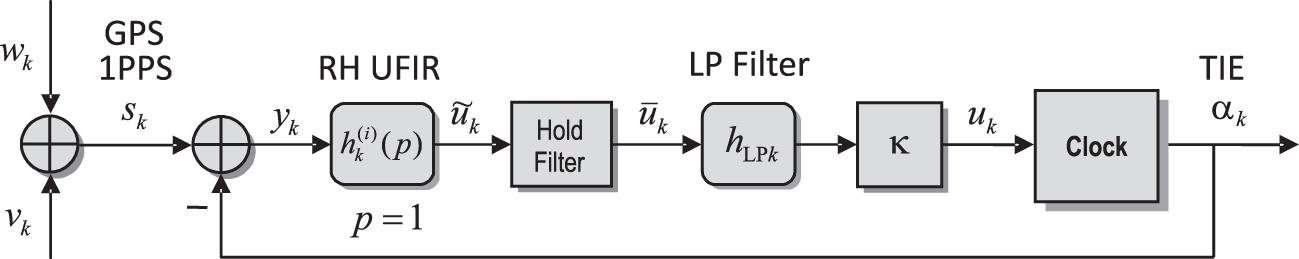
Figure 11.3 Loop model of local clock synchronization based on GPS 1PPS timing signals.
11.2.1 Clock Digital Synchronization Loop
The clock synchronization loop proposed in [11] is shown in Fig. 11.3. The GPS 1PPS timing signal ![]() is represented with the GPS time uncertainty (or disturbance)
is represented with the GPS time uncertainty (or disturbance) ![]() caused by different satellites in a view and some other random factors. It is also complicated by the uniformly distributed sawtooth noise
caused by different satellites in a view and some other random factors. It is also complicated by the uniformly distributed sawtooth noise ![]() , whose values range from
, whose values range from ![]() to
to ![]() owing to the principle of the 1PPS signal formation. Typical examples of the GPS 1PPS signal errors are given in Fig. 11.4 [11]. Random
owing to the principle of the 1PPS signal formation. Typical examples of the GPS 1PPS signal errors are given in Fig. 11.4 [11]. Random ![]() (Fig. 11.4a) ranges closer to zero than the sawtooth noise
(Fig. 11.4a) ranges closer to zero than the sawtooth noise ![]() , which is uniformly distributed within
, which is uniformly distributed within ![]() in ns (Fig. 11.4b). Errors in the GPS 1PPS timing signal shown in Fig. 11.4c are caused by a mixture of
in ns (Fig. 11.4b). Errors in the GPS 1PPS timing signal shown in Fig. 11.4c are caused by a mixture of ![]() and
and ![]() . In some GPS timing receivers, a negative sawtooth correction code is available in the protocol. If this code is applied, the 1PPS signal error becomes approximately
. In some GPS timing receivers, a negative sawtooth correction code is available in the protocol. If this code is applied, the 1PPS signal error becomes approximately ![]() .
.
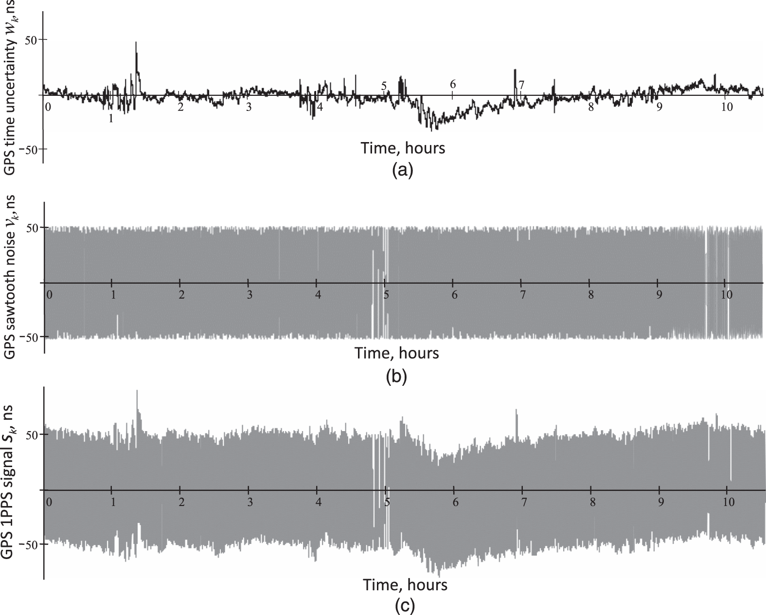
Figure 11.4 Typical errors in GPS timing receivers: (a) GPS time uncertainty  caused by different satellites in a view and other random factors, (b) sawtooth noise
  induced by the receiver, and (c) time error
  in the GPS 1PPS reference signal.

Figure 11.5 A typical function of a nonstationary TIE  of an unlocked crystal clock.
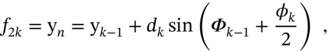
A typical function of a nonstationary TIE ![]() of an unlocked crystal clock is shown in Fig. 11.5 [11]. The synchronization loop requires
of an unlocked crystal clock is shown in Fig. 11.5 [11]. The synchronization loop requires ![]() neighboring past data points, from
neighboring past data points, from ![]() to
to ![]() , and operates as follows. The TIE
, and operates as follows. The TIE ![]() is measured relative to
is measured relative to ![]() by the TIE counter, and the difference signal
by the TIE counter, and the difference signal ![]() is computed. To predict the disciplining signal
is computed. To predict the disciplining signal ![]() at the current point
at the current point ![]() , the RH UFIR filter is used, which has an impulse response of the
, the RH UFIR filter is used, which has an impulse response of the ![]() th degree
th degree ![]() . The predicted value
. The predicted value ![]() is held as
is held as ![]() by the hold filter, smoothed by the LP filter with the impulse response
by the hold filter, smoothed by the LP filter with the impulse response ![]() , and scaled with
, and scaled with ![]() to obtain the necessary control signal
to obtain the necessary control signal ![]() , which disciplines the clock.
, which disciplines the clock.
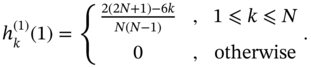
The ramp RH UFIR filter of the first degree, ![]() and
and ![]() , is used with the impulse response function originally derived in [71],
, is used with the impulse response function originally derived in [71],
The 1‐step predictive filtering estimate is obtained as
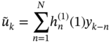
by the discrete convolution using data ![]() taken from
taken from ![]() .
.
To hold ![]() over time to continuously steer the clock between suboptimally defined values, a hold filter is used such that
over time to continuously steer the clock between suboptimally defined values, a hold filter is used such that
where ![]() is an integer part of
is an integer part of ![]() . By (11.13), the input and output values of the hold filter become equal when
. By (11.13), the input and output values of the hold filter become equal when ![]() is multiple to
is multiple to ![]() . Between two such adjacent points, the output value of the hold filter is constant.
. Between two such adjacent points, the output value of the hold filter is constant.
For multiple clock steering with period ![]() , where
, where ![]() is the sampling time and
is the sampling time and ![]() is the number of sampling intervals, the hold filter produces a step signal
is the number of sampling intervals, the hold filter produces a step signal ![]() . Applied directly to the clock,
. Applied directly to the clock, ![]() guarantees suboptimal steering and assures that
guarantees suboptimal steering and assures that ![]() ranges within narrow bounds around zero. On the other hand, the stepwise
ranges within narrow bounds around zero. On the other hand, the stepwise ![]() may not guarantee the required clock performance.
may not guarantee the required clock performance.
To smooth ![]() , an LP filter with the impulse response
, an LP filter with the impulse response ![]() is used. It has been shown in [11] experimentally that the 1‐order LP filter with the impulse response
is used. It has been shown in [11] experimentally that the 1‐order LP filter with the impulse response

where ![]() is the filter time constant and
is the filter time constant and ![]() , is able to fit the demands for precise clock synchronization. Finally, the gain
, is able to fit the demands for precise clock synchronization. Finally, the gain ![]() is applied to produce the control signal
is applied to produce the control signal ![]() and provide steering of clock errors.
and provide steering of clock errors.
Experimental Verification
Experimental investigations of the synchronization loop shown in Fig. 11.3 were provided in [11]. To outline the capabilities of FIR state estimators in practical applications, next we present only the most typical characteristics of a steered clock with an oven‐controlled crystal oscillator (OCXO). The clock errors are presented in terms of the Allan deviation and precision time protocol (PTP) variance for ![]() ,
, ![]() , and
, and ![]() . The optimal horizon
. The optimal horizon ![]() and optimal time constant
and optimal time constant ![]() are measured experimentally by minimizing the MSE relative to the TIE of an OCXO‐based clock with and without the sawtooth. For GPS 1PPS signal with sawtooth, the optimal horizon was measured as
are measured experimentally by minimizing the MSE relative to the TIE of an OCXO‐based clock with and without the sawtooth. For GPS 1PPS signal with sawtooth, the optimal horizon was measured as ![]() and without the sawtooth as
and without the sawtooth as ![]() . More details about this loop can be found in [11].
. More details about this loop can be found in [11].
![Schematic illustration of allan deviation of the GPS-locked OCXO-based clock for different T,s of the 1-order LP filter. GPS 1PPS signal has sawtooth and Nopt=250 [11].](https://imgdetail.ebookreading.net/2023/10/9781119863076/9781119863076__9781119863076__files__images__c11f006.png)
Figure 11.6 Allan deviation of the GPS‐locked OCXO‐based clock for different  of the 1‐order LP filter. GPS 1PPS signal has sawtooth and
  [11].
[11].
Allan Deviation
The Allan deviation of a locked OCXO‐based clock was investigated in [11] as a function of the LP filter time constant ![]() . It follows from Fig. 11.6 that the Allan deviation of the 1PPS signal with sawtooth ranges higher than that of the OCXO‐based clock when the averaging time
. It follows from Fig. 11.6 that the Allan deviation of the 1PPS signal with sawtooth ranges higher than that of the OCXO‐based clock when the averaging time ![]() is less than about 5000 sec. The suboptimal UFIR filter removes the sawtooth, improves the performance, and makes it such that the Allan deviation remains large only when
is less than about 5000 sec. The suboptimal UFIR filter removes the sawtooth, improves the performance, and makes it such that the Allan deviation remains large only when ![]() . Further improvement is achieved using an LP filter, which dramatically reduces the Allan deviation to the level of an OCXO‐based clock. Figure 11.6 suggests that
. Further improvement is achieved using an LP filter, which dramatically reduces the Allan deviation to the level of an OCXO‐based clock. Figure 11.6 suggests that ![]() can be accepted as near optimal. Indeed, with small
can be accepted as near optimal. Indeed, with small ![]() the Allan deviation value is due to the unlocked clock and with large
the Allan deviation value is due to the unlocked clock and with large ![]() due to the UFIR filter (or sawtooth‐less measurements). The LP filter causes an excursion, who peak value reaches a minimum when
due to the UFIR filter (or sawtooth‐less measurements). The LP filter causes an excursion, who peak value reaches a minimum when ![]() , it grows and shifts to the right when
, it grows and shifts to the right when ![]() , and it grows and shifts to the left if
, and it grows and shifts to the left if ![]() .
.
Precision Time Protocol Variance
Another measure of clock errors is the PTV variance. It is worth noting as a matter of notation that by ![]() the square root of PTP variance
the square root of PTP variance ![]() is equal to the time deviation (TDEV) specified in [78]. The PTP variance relates to the Allan variance
is equal to the time deviation (TDEV) specified in [78]. The PTP variance relates to the Allan variance ![]() as
as ![]() , and [76] states that this is the main measure of locked clock errors.
, and [76] states that this is the main measure of locked clock errors.
The improvement in PTP variance for a GPS 1PPS signal measured without a sawtooth is illustrated in Fig. 11.7, where the recommended boundary (dashed) is taken from [78].
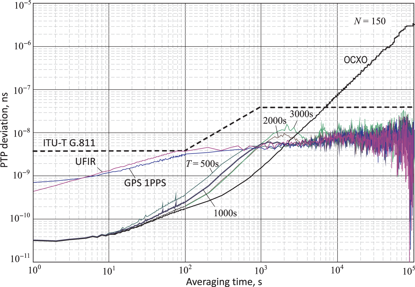
Figure 11.7 PTP deviation of a GPS locked crystal clock for different  of the 1‐order LP filter and
  over GPS 1PPS signal without the sawtooth.
As can be seen, the PTP deviation of an OCXO‐based clock exceeds the recommended boundary when ![]() . The PTP deviation of the GPS 1PPS signal without the sawtooth ranges very close to the UFIR filter output, and it follows that the UFIR filter removes the sawtooth very efficiently. Both these measures range below the recommended boundary and approach it when
. The PTP deviation of the GPS 1PPS signal without the sawtooth ranges very close to the UFIR filter output, and it follows that the UFIR filter removes the sawtooth very efficiently. Both these measures range below the recommended boundary and approach it when ![]() . The LP filter significantly improves the performance and reduces the clock PTP deviation by a factor of 10 or more over the recommended boundary. It also follows that a near optimal time constant can be accepted as
. The LP filter significantly improves the performance and reduces the clock PTP deviation by a factor of 10 or more over the recommended boundary. It also follows that a near optimal time constant can be accepted as ![]() .
.
In general, the fact remains: the iterative UFIR filtering Algorithm 11 is an efficient tool for GPS‐based clock steering, since the KF is not suitable for filtering flicker noise components.
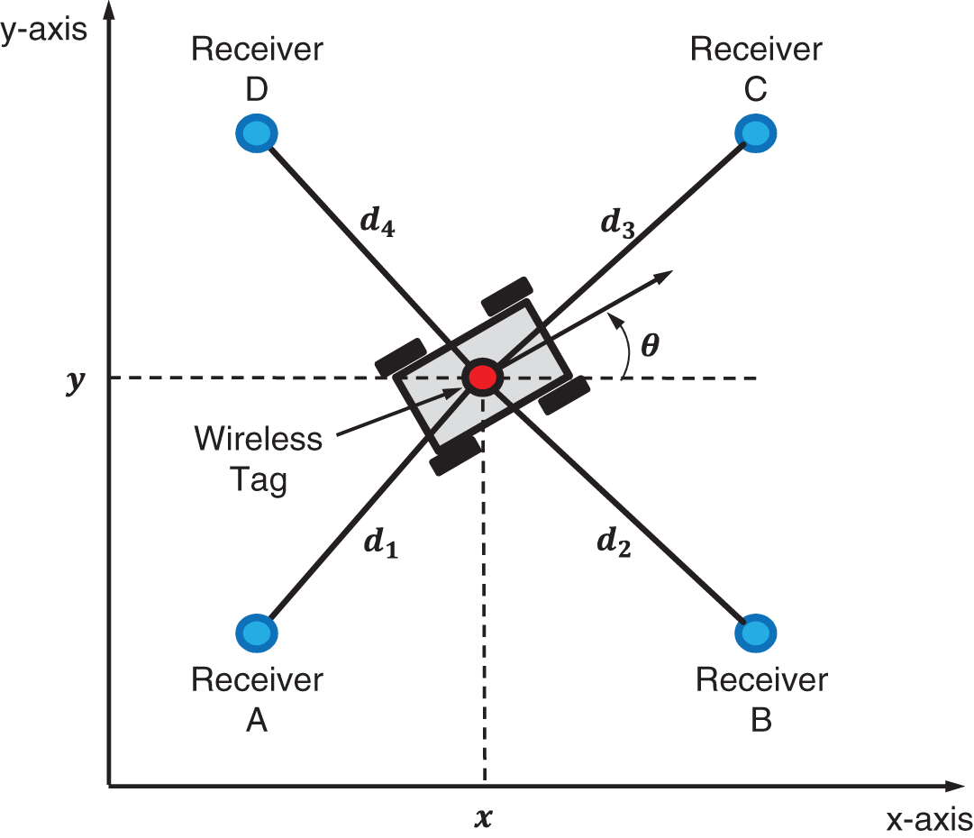
Figure 11.8 2‐D schematic geometry of the mobile robot localization.
11.3 Localization Over WSNs Using Particle/UFIR Filter
A well‐known disadvantage of the PF‐based localization of maneuvering objects is the need to generate a large number of particles in order to avoid divergence. The process requires resampling, which assumes that particles with higher weights (i.e., high likelihoods) will be statistically selected many times. This leads to a loss of diversity among the particles so that the resultant set will contain many repeated particles. The effect is known as sample impoverishment and usually occurs when the noise is not intensive or the number of particles is small.
To make the PF‐based localization more reliable by avoiding the divergence, the PF was combined in [143] with the UFIR filter. In the proposed hybrid PF/UFIR structure, the PF plays the role of the main filter, and the UFIR filter is used as the supporting filter. The PF estimates the state in normal situations, when there is sample impoverishment and no failures. Otherwise, when the PF fails, the UFIR filter restarts it.
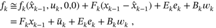
This hybrid structure was used in [143] to provide indoor mobile robot localization using a wireless tag with a transmitter, four receivers, and a server computer as shown in Fig. 11.8. A wireless tag attached to the mobile robot transmits a signal to four receivers deployed at exactly known coordinates. The clocks of the receivers are synchronized using the synchronization line. Distances between the tag and the receivers are measured via time‐of‐arrival (TOA). The TOA data are transferred to the server computer to generate time‐difference‐of‐arrival (TDOA) measurements, which are represented by the following equation,

where ![]() ,
, ![]() , and
, and ![]() are the TDOA data (in units of nanoseconds) and
are the TDOA data (in units of nanoseconds) and ![]() is the speed of light. Here,
is the speed of light. Here, ![]() ,
, ![]() , is the
, is the ![]() th distances between the mobile robot and the receivers. The distances are coupled with the robot local coordinates
th distances between the mobile robot and the receivers. The distances are coupled with the robot local coordinates ![]() and
and ![]() and the
and the ![]() th receiver constant coordinates
th receiver constant coordinates ![]() and
and ![]() by four nonlinear equations for
by four nonlinear equations for ![]() ,
,
At the current point ![]() , the mobile robot pose is given by the state vector
, the mobile robot pose is given by the state vector ![]() , where
, where ![]() is a heading angle in the 2D plane local coordinates. Motion of the mobile robot is adjusted by the control signal
is a heading angle in the 2D plane local coordinates. Motion of the mobile robot is adjusted by the control signal ![]() , where
, where ![]() is the incremental distance (in meters) and
is the incremental distance (in meters) and ![]() is the incremental change in the heading angle (in degrees). The following difference equations represent the dynamics of the robot's movement,
is the incremental change in the heading angle (in degrees). The following difference equations represent the dynamics of the robot's movement,
The robot is equipped with a fiber optic gyroscope (FOG), which directly measures ![]() , and the fourth required measurement becomes
, and the fourth required measurement becomes
Combined the measurements, the observation vector is constructed as ![]() . Finally, the state equation
. Finally, the state equation ![]() and observation equation
and observation equation ![]() formalize the localization problem in state space with
formalize the localization problem in state space with
where the process noise ![]() and measurement noise
and measurement noise ![]() have the covariances
have the covariances ![]() and
and ![]() . Given (11.21) and (11.22), the mobile robot coordinates and heading are estimated by the PF.
. Given (11.21) and (11.22), the mobile robot coordinates and heading are estimated by the PF.
11.3.1 Sample Impoverishment Issue
The PF‐based approach assumes that the robot coordinates are the first‐order Markov processes evolving from one point to another with known initial and transition distributions and that the conditionally independent observations depend only on the robot position. To estimate ![]() ,
, ![]() , and
, and ![]() , the PF generates a set of samples at each
, the PF generates a set of samples at each ![]() that approximates the distributions of the coordinates conditioned on all past observations. This process is called resampling and causes an issue known as sample impoverishment.
that approximates the distributions of the coordinates conditioned on all past observations. This process is called resampling and causes an issue known as sample impoverishment.
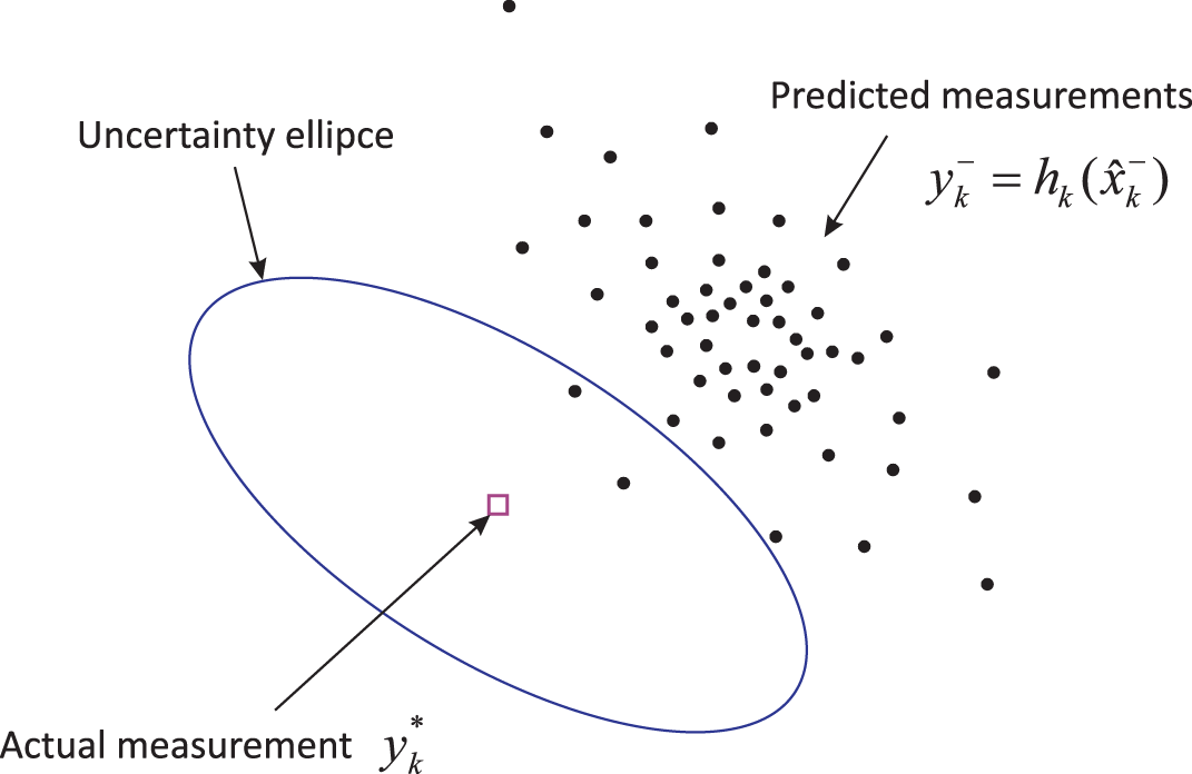
Figure 11.9 A typical scenario with the sample impoverishment.
Figure 11.9 illustrates an idea of sample impoverishment in a typical scenario. The ![]() th dot,
th dot, ![]() , represents a sample of the
, represents a sample of the ![]() th predicted measurement
th predicted measurement ![]() defined by
defined by
where ![]() is the
is the ![]() th a priori particle (i.e., sample of the a priori estimated state) and
th a priori particle (i.e., sample of the a priori estimated state) and ![]() is the number of the particles. In the Gaussian approximation, the likelihood (i.e., weight) of each particle is a reciprocal of the difference between the actual measurement
is the number of the particles. In the Gaussian approximation, the likelihood (i.e., weight) of each particle is a reciprocal of the difference between the actual measurement ![]() and the predicted measurement. Therefore, the closer the samples of the predicted measurement
and the predicted measurement. Therefore, the closer the samples of the predicted measurement ![]() are to
are to ![]() , the higher the weights of the corresponding a priori particles.
, the higher the weights of the corresponding a priori particles.
In the example shown in Fig. 11.9, there are only two samples of predicted measurements within the measurement: uncertainty or error ellipse. Thus, only these particles will receive significant weights, and resampling will repeat them many times as the a posteriori particles ![]() . As a consequence, sample impoverishment and failures will occur. The problem is mainly associated with low‐intensity process noise and/or measurement noise and/or the small number of particles required to ensure fast localization. Other factors can also cause sample impoverishment. Therefore, a great deal of efforts may be required to satisfactorily address the problem. But despite all efforts, the problem remains fundamental, and it is impossible to completely avoid sample impoverishment.
. As a consequence, sample impoverishment and failures will occur. The problem is mainly associated with low‐intensity process noise and/or measurement noise and/or the small number of particles required to ensure fast localization. Other factors can also cause sample impoverishment. Therefore, a great deal of efforts may be required to satisfactorily address the problem. But despite all efforts, the problem remains fundamental, and it is impossible to completely avoid sample impoverishment.
11.3.2 Hybrid Particle/UFIR Filter
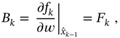
To improve localization accuracy, PF has been combined in [143] with an EFIR filter in a hybrid algorithm that encompasses two key procedures: 1) detection of PF failures and 2) particles regeneration and PF resetting. PF fault detection is organized in a diagnosis algorithm using Mahalanobis distance. To regenerate new particles and reset PF, an EFIR filter is used to obtain the state estimates when the PF fails. The choice of an EFIR filter that is robust and BIBO stable was made in attempts to fulfil a basic requirement: an auxiliary filter does not have to be obligatorily accurate, but it has to be robust and stable. Note that resetting the PF with an EFIR filter instead of generating a lot particles solves another critical issue: reducing the computational complexity and time required for real‐time localization.
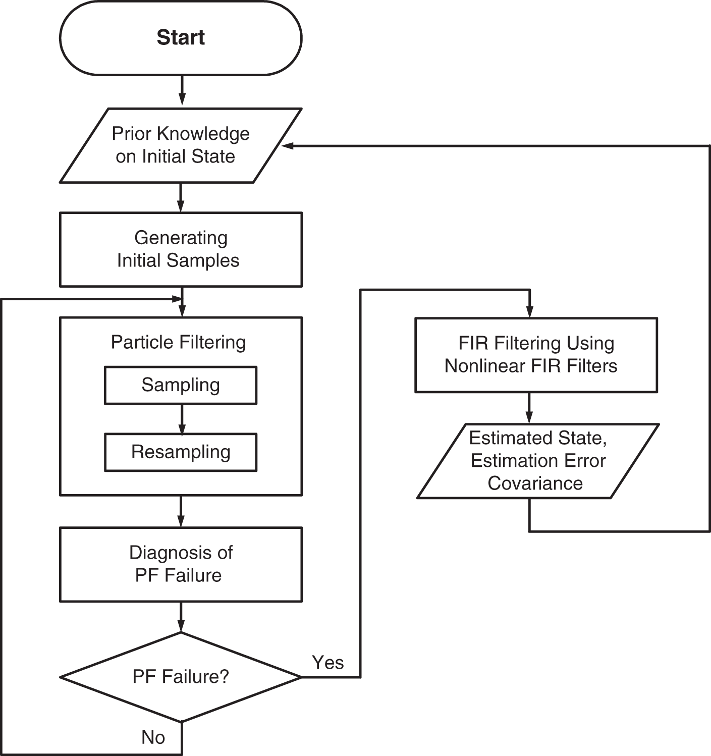
Figure 11.10 A flowchart of the hybrid PF/EFIR algorithm.
A flowchart of the hybrid PF/EFIR algorithm is given in Fig. 11.10. PF plays the role of the main filter, which provides estimates of the mobile robot coordinates and heading under normal conditions. Diagnostics of PF failures is performed continuously, and when the PF fails, the auxiliary EFIR filter provides information to reset the failed PF. Erroneous estimates at the PF output are detected taking into account the following features of sample impoverishment: 1) only a few predicted samples fall into the uncertainty ellipse, and 2) the predicted samples are usually far from actual measurement. PF rejections are detected by checking the number of samples within the uncertainty ellipse using the Mahalanobis distance.
This example provides further evidence of the effectiveness of hybrid filters in solving the localization problem.
11.4 Self‐Localization Over RFID Tag Grids
Radio frequency identification (RFID) tag‐based networks and grids are designed to organize self‐localization of various moving objects in GPS‐denied indoor environments. Each tag has an ID number corresponding to a unique location and can be either active or passive. To increase awareness, information describing a local 2D or 3D surrounding can be programmed in each tag and delivered to users by request. The method is low cost and available for any purpose, provided the communication between a target and the tags. However, since low‐cost measurements are usually very noisy, optimal estimators are required.

Figure 11.12 2D schematic geometry of a vehicle traveling on an indoor floorspace nested with two RFID tags, T1 and T2, having exactly known coordinates.
An example of the 2D schematic geometry of a vehicle traveling on an indoor floorspace nested with two RFID tags ![]() and
and ![]() (the number can be arbitrary) having exactly known coordinates is shown in Fig. 11.12 [149,150]. The vehicle reader measures the distances to the tags, and the heading angle
(the number can be arbitrary) having exactly known coordinates is shown in Fig. 11.12 [149,150]. The vehicle reader measures the distances to the tags, and the heading angle ![]() is measured using a fiber‐optic gyroscope (FOG); subfigures (a) and (b) are used when the vehicle and the tags are not in the same plane. The vehicle travels in direction
is measured using a fiber‐optic gyroscope (FOG); subfigures (a) and (b) are used when the vehicle and the tags are not in the same plane. The vehicle travels in direction ![]() , and its trajectory is controlled by the left and right wheels. The incremental distances that the vehicle travels on these wheels are
, and its trajectory is controlled by the left and right wheels. The incremental distances that the vehicle travels on these wheels are ![]() and
and ![]() , respectively. The distance between the left and right wheels is
, respectively. The distance between the left and right wheels is ![]() , and the stabilized wheel is not shown. The vehicle moves in its own planar Cartesian coordinates
, and the stabilized wheel is not shown. The vehicle moves in its own planar Cartesian coordinates ![]() with a center at
with a center at ![]() ; that is, the vehicle direction always coincides with axis
; that is, the vehicle direction always coincides with axis ![]() . The FOG measures
. The FOG measures ![]() directly.
directly.
The indoor space is commonly nested with ![]() RFID tags
RFID tags ![]() ,
, ![]() , where coordinates
, where coordinates ![]() of the
of the ![]() th tag are exactly known. It is supposed that at each
th tag are exactly known. It is supposed that at each ![]() the vehicle reader can simultaneously detect
the vehicle reader can simultaneously detect ![]() tags, where the number
tags, where the number ![]() varies over time, and measures the distance
varies over time, and measures the distance ![]() to the
to the ![]() th tag, where
th tag, where ![]() , which can be any of the nested tags.
, which can be any of the nested tags.
Referring to Fig. 11.12 and vehicle odometry, the incremental distance ![]() and heading angle
and heading angle ![]() can be found as
can be found as
and the vehicle coordinates ![]() and
and ![]() and heading
and heading ![]() obtained by the vehicle kinematics using equations
obtained by the vehicle kinematics using equations

where ![]() ,
, ![]() , and
, and ![]() are projected to
are projected to ![]() via the incremental distances
via the incremental distances ![]() and
and ![]() . Note that all these values are practically not exact and undergo random variations.
. Note that all these values are practically not exact and undergo random variations.
11.4.1 State‐Space Localization Problem
To solve the localization problem in state space, the state vector can be assigned as ![]() and the input vector as
and the input vector as ![]() . Random additive components in these vectors can be supposed to be
. Random additive components in these vectors can be supposed to be ![]() and
and ![]() . The nonlinear state equation thus becomes
. The nonlinear state equation thus becomes
where the nonlinear function ![]() is combined with components given by (11.27)–(11.29).
is combined with components given by (11.27)–(11.29).
The measurement equations can be written as

By introducing the observation vector ![]() , nonlinear function
, nonlinear function ![]() , and measurement noise
, and measurement noise ![]() , the observation equation can be rewritten in a compact form as
, the observation equation can be rewritten in a compact form as
where noise ![]() has the covariance
has the covariance ![]() .
.
Extended State‐Space Model
The standard procedure (3.228) applied to function ![]() gives the first‐order approximation
gives the first‐order approximation
where ![]() is an estimate at
is an estimate at ![]() ,
, ![]() is known, and
is known, and ![]() ,
, ![]() , and
, and ![]() are Jacobian matrices defined by
are Jacobian matrices defined by


where ![]() and
and ![]() .
.
By applying (3.229) to ![]() , the first‐order approximation becomes
, the first‐order approximation becomes
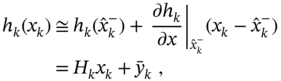
where ![]() is known and
is known and ![]() is a Jacobian matrix defined by
is a Jacobian matrix defined by

where ![]() ,
, ![]() .
.
The first‐order extended state‐space model can therefore be written as
where ![]() and
and ![]() have the covariances
have the covariances ![]() and
and ![]() .
.
11.4.2 Localization Performance
Provided the approximation (11.38) and (11.39), the EKF algorithm (3.240)–(3.244) and EFIR Algorithm 15 can be directly applied to organize self‐localization as shown next.
Consider a robot platform moving down an aisle in an RFID grid environment where tags are nested in the floor and ceiling (Fig. 11.13) [150].
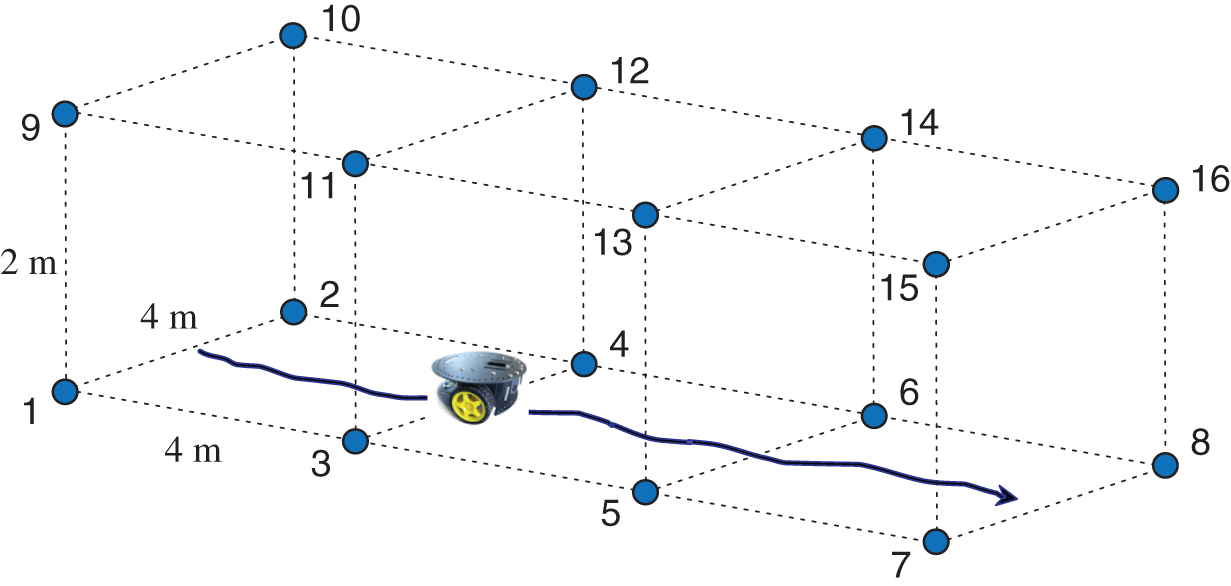
Figure 11.13 Schematic diagram of a vehicle platform traveling on an indoor passway in the RFID tag environment with eight tags mounted on a ceiling and eight tags mounted on a floor.
The environment is simple because the coordinates of a tag can be easily calculated based on its geometrical position. It is supposed that the reader is able to detect eight tags at the same time at each floorspace point, but some tags may not be available due to faults, furniture isolation, low‐power consumption, etc. However, at least two tags are always available.
To assess the quality of localization, noise was generated in [150] with the following standard deviations: ![]() ,
, ![]() , and
, and ![]() . Since the tags on the ceiling are farthest from the platform, the standard deviations of the measurement noise are set as
. Since the tags on the ceiling are farthest from the platform, the standard deviations of the measurement noise are set as ![]() ,
, ![]() , and
, and ![]() . The optimal horizon is measured as
. The optimal horizon is measured as ![]() . The tags detected in 6 intervals (in m) along the passway are listed in Table 11.1, where tags 12 and 14–16 are not available.
. The tags detected in 6 intervals (in m) along the passway are listed in Table 11.1, where tags 12 and 14–16 are not available.
Table 11.1 Tags detected in six intervals (in m) along a passway shown in Fig. 11.13; tags 12 and 14–16 were not available.
| m | Tag | |||||||||||
|---|---|---|---|---|---|---|---|---|---|---|---|---|
| 1 | 2 | 3 | 4 | 5 | 6 | 7 | 8 | 9 | 10 | 11 | 13 | |
| 0–2 | x | x | – | – | – | – | – | – | x | x | – | – |
| 2–4 | x | x | x | – | – | – | – | – | x | x | – | – |
| 4–6 | – | – | x | x | – | – | – | – | – | – | x | – |
| 6–8 | – | – | x | – | x | x | – | – | – | – | – | x |
| 8–10 | – | – | – | – | x | x | – | – | – | – | – | x |
| 10–12 | – | – | – | – | – | – | x | x | – | – | – | – |
Since noise statistics are typically not known exactly, an error factor ![]() was introduced such that
was introduced such that ![]() makes the case ideal and the noise covariances were replaced in the algorithms by
makes the case ideal and the noise covariances were replaced in the algorithms by ![]() ,
, ![]() , and
, and ![]() . It has been shown that under ideal conditions,
. It has been shown that under ideal conditions, ![]() , the EKF and EFIR filter give very consistent estimates and are not prone to divergence. The situation changes dramatically for
, the EKF and EFIR filter give very consistent estimates and are not prone to divergence. The situation changes dramatically for ![]() , which leads to the errors shown in Fig. 11.14. Indeed, for tag sets taken from Table 11.1 with three different realisations of the same noise, EKF demonstrates: (a) local instability, (b) single divergence, and (c) multiple divergence. In contrast, the EFIR filter turned out to be much more stable with no signs of divergence.
, which leads to the errors shown in Fig. 11.14. Indeed, for tag sets taken from Table 11.1 with three different realisations of the same noise, EKF demonstrates: (a) local instability, (b) single divergence, and (c) multiple divergence. In contrast, the EFIR filter turned out to be much more stable with no signs of divergence.
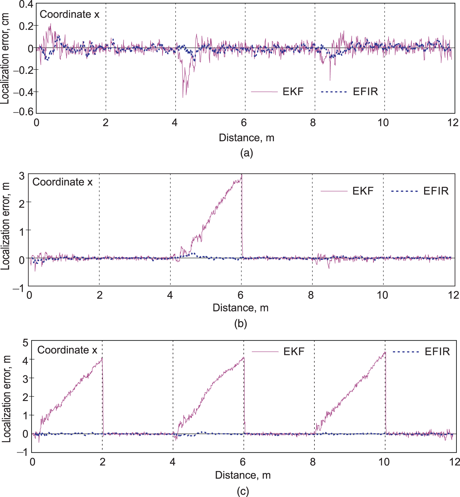
Figure 11.14 Localization errors caused by imprecisely known noise covariances for  : (a) local instabilities, (b) single divergence of EKF, and (c) multiple divergence of EKF.
This investigation clearly points to another possible source of divergence in the EKF, namely, errors in the noise covariances. It also shows that increasing the number of tags interacting with the platform protects EKF from divergency so that massively nested tags can guarantee localization stability.
11.5 INS/UWB‐Based Quadrotor Localization
One of the most useful modern innovations is an unmanned aerial vehicle called a quadcopter or quadrotor. Due to the ability to fulfil tasks traditionally assigned to humans, quadrotors have became irreplaceable in many branches of modern life. A prerequisite for a quadrotor to complete various tasks is accurate position information, which must be retrieved quickly and preferably optimally with sufficient robustness in complex, harsh, and volatile navigation environments.
A typical quadrotor localization scheme that combines the capabilities of an inertial navigation system (INS) and ultra wide band (UWB)–based system is shown in Fig. 11.15 [217]. A navigation environment has been created here with multiple reference nodes (RNs), and the UWB and INS units are installed on the quadrotor. The UWB‐based subsystem derives the quadrotor position ![]() in the east direction
in the east direction ![]() , north direction
, north direction ![]() , and vertical direction
, and vertical direction ![]() via distances
via distances ![]() measured between the
measured between the ![]() th RN and a quadrotor. The INS‐based subsystem obtains the quadrotor position
th RN and a quadrotor. The INS‐based subsystem obtains the quadrotor position ![]() . Provided
. Provided ![]() and
and ![]() , the difference
, the difference ![]() is estimated to correct the INS position
is estimated to correct the INS position ![]() and produce finally the position vector
and produce finally the position vector ![]() .
.
![Schematic illustration of iNS/UWB-integrated quadrotor localization scheme [217].](https://imgdetail.ebookreading.net/2023/10/9781119863076/9781119863076__9781119863076__files__images__c11f015.png)
Figure 11.15 INS/UWB‐integrated quadrotor localization scheme [217].
A specific feature of this system is that UWB data are contaminated with CMN in all of the directions as shown in Fig. 11.16. Thus, the white Gaussian approximation may not be sufficient for accurate quadrotor localization, and the GKF algorithm (3.146)–(3.151) or UFIR filtering Algorithm 13 should be applied.

Figure 11.16 CMN in UWB‐derived data: (a) east direction, (b) north direction, and (c) vertical direction.
11.5.1 Quadrotor State Space Model Under CMN
Based on the scheme shown in Fig. 11.15, the quadrotor dynamics can be represented with increments in the coordinates ![]() ,
, ![]() , and
, and ![]() and velocities
and velocities ![]() ,
, ![]() , and
, and ![]() , which can then be united in the state equation
, which can then be united in the state equation
where

![]() is the time step, and
is the time step, and ![]() .
.
For ![]() representing measurements, the observation equation becomes
representing measurements, the observation equation becomes
where

where ![]() is the CMN (Fig. 11.16) represented with the Gauss‐Markov model
is the CMN (Fig. 11.16) represented with the Gauss‐Markov model
in which ![]() is the coloredness factor matrix such that
is the coloredness factor matrix such that ![]() remains stationary and noise
remains stationary and noise ![]() has the covariance
has the covariance ![]() .
.
To apply the GKF and general UFIR filter, the measurement difference is introduced and transformed as

where ![]() ,
, ![]() , and white Gaussian
, and white Gaussian ![]() has the the covariance
has the the covariance
where ![]() . For this model, the measurement residual
. For this model, the measurement residual ![]() is given by
is given by
where ![]() . Since the cross covariance transforms to
. Since the cross covariance transforms to
and ![]() is the prior error covariance, the innovation error covariance
is the prior error covariance, the innovation error covariance ![]() becomes
becomes

With the previous modifications, the general UFIR filtering Algorithm 13 can be applied straightforwardly. To apply the GKF algorithm (3.160)–(3.165), noise vectors ![]() and
and ![]() must be de‐correlated. Alternatively, to apply the GKF algorithm (3.146)–(3.151), a new optimal Kalman gain must be derived for time‐correlated noise.
must be de‐correlated. Alternatively, to apply the GKF algorithm (3.146)–(3.151), a new optimal Kalman gain must be derived for time‐correlated noise.
11.5.2 Localization Performance
Tuning localization algorithms is an important process, which does not always end successfully due to the practical inability of measuring noise statistics in real time. To obtain reliable estimates over data arriving with a time step of ![]() , the best and worst cases were considered in [217].
, the best and worst cases were considered in [217].
Best Case: For the average quadrotor velocity of ![]() estimated with a tolerance of 20%, the noise standard deviation is set as
estimated with a tolerance of 20%, the noise standard deviation is set as ![]() . Noise in the first state is ignored, and the system noise covariance is specified with
. Noise in the first state is ignored, and the system noise covariance is specified with

The average noise variances in UWB data are measured as ![]() ,
, ![]() , and
, and ![]() . Accordingly, the measurement noise covariance is set as
. Accordingly, the measurement noise covariance is set as ![]() . Experimentally, minimum localization errors were obtained by the optimal coloredness factor
. Experimentally, minimum localization errors were obtained by the optimal coloredness factor ![]() .
.
Worst Case: Since the actual quadrotor velocity can vary by several times and the variance of UWB noise can be several times larger than in individual measurements, the error factor ![]() was introduced as
was introduced as ![]() and
and ![]() , and it was supposed that in the worst case
, and it was supposed that in the worst case ![]() covers most of practical situations.
covers most of practical situations.

Figure 11.17 RMSEs produced by the KF, cKF, UFIR filter, and cUFIR filter. For the UWB boundary, filtering errors should be as low as possible.
In this experiment, a quadrotor travels along a planned path considered as a reference trajectory. Typical RMSEs produced by the KF, GKF developed for CMN (cKF), UFIR filter, and general UFIR filter developed for CMN (cUFIR) are sketched in Fig. 11.17 along with the UWB error boundary. For this boundary, filtering errors should be as low as possible. What this experiment de facto reveals is that the properly tuned cKF is most accurate in the best case, but less accurate in the worst case. The cKF is also most sensitive to errors in the noise covariances, and its RMSE crosses the UWB boundary when ![]() . The latter means that the more accurate cKF is less robust than the original KF. Thereby, this experiment confirms the earlier made conclusion that an increase in the estimation accuracy is achieved using additional tuning factors at the expanse of robustness. It is also seen that both UFIR filters are robust against changes in
. The latter means that the more accurate cKF is less robust than the original KF. Thereby, this experiment confirms the earlier made conclusion that an increase in the estimation accuracy is achieved using additional tuning factors at the expanse of robustness. It is also seen that both UFIR filters are robust against changes in ![]() and are reasonably accurate since their RMSEs do not exceed the UWB boundary.
and are reasonably accurate since their RMSEs do not exceed the UWB boundary.
11.6 Processing of Biosignals
Advances in sensor technology in recent decades have extended digital technologies to electrical and mechanical signals generated by the human body and referred to as biosignals. Such signals can be measured with or without contact with the body and are useful in a wide range of medical applications, from diagnostics and remote monitoring to effective prosthesis control. The best‐known bioelectrical signals are: electrocardiogram (ECG), electromyogram (EMG), electroencephalogram, mechanomyogram, electrooculography, galvanic skin response, and magnetoencephalogram. Depending on the nature of the origin, biosignals can be quasiperiodic, like an ECG, or impulsive, like an EMG.
Since biosignals are generated by the body at low electrical levels, their measurements are accompanied by intense noise of little‐studied origin. Another important specificity is that biosignals, as a rule, do not have simple models. Therefore, methods for optimal processing of biosignals are usually based on assumptions that cannot be theoretically substantiated, as in artificial intelligence. To illustrate possible extensions of the state estimation methods to biosignals, next we will consider examples of ECG and EMG biosignals and solve specific problems using Kalman and UFIR estimators.
11.6.1 ECG Signal Denoising Using UFIR Smoothing
The ECG signals allow detecting a wide variety of heart diseases. Since heartbeats may vary slightly from each other, accurate measurements are required. This is particularly important when data are used to extract ECG features and make decisions about the heart state using special software. Various types of noises contaminate the ECG signal during its acquisition and transmission, such as high frequency noise (electromyogram noise, additive Gaussian noise, and power line interference) and low frequency noise (baseline wandering). Because noise can cause misinterpretation of the heart state, efficient denoising is required.

Figure 11.18 Single ECG pulse measured in the presence of noise (Data). Noise reduction is provided by an UFIR smoother of degree  .
.
A typical measured heartbeat pulse (Data) is shown in Fig. 11.18, where one can recognize the central rapid excursions, commonly referred to as the QRS‐complex, slow left excursion (T‐wave), slow first right excursion (T‐wave), and slow second right excursion (U‐wave). This suggests that the ECG signal mostly changes slow over time and is highly oversampled, with the exception of the QRS region, where it is critically sampled. Thus, in the frequency domain, the ECG signal energy is concentrated in two bands: low frequencies associated with LP filtering and high frequencies with BP filtering. By using the ![]() th degree
th degree ![]() ‐lag UFIR smoother, suboptimal denoising of the slow part can be provided on the large horizon
‐lag UFIR smoother, suboptimal denoising of the slow part can be provided on the large horizon ![]() , while the critically sampled fast excursions in the QRS‐complex require the shortest possible horizon
, while the critically sampled fast excursions in the QRS‐complex require the shortest possible horizon ![]() to avoid output bias. To enable universal noise cancellation, an adaptive iterative
to avoid output bias. To enable universal noise cancellation, an adaptive iterative ![]() ‐lag UFIR smoothing algorithm has been designed in [108].
‐lag UFIR smoothing algorithm has been designed in [108].
Adaptive Smoothing of ECG Data
To adaptively remove noise from ECG data using an UFIR smoother, a window ![]() is assigned to cover the QRS‐complex as shown in Fig. 11.18. Since points Q and S are well detectable in the ECG pulse, the window boundaries are assigned as
is assigned to cover the QRS‐complex as shown in Fig. 11.18. Since points Q and S are well detectable in the ECG pulse, the window boundaries are assigned as ![]() and
and ![]() . The horizon
. The horizon ![]() is measured by removing the QRS‐complex. By determining
is measured by removing the QRS‐complex. By determining ![]() ,
, ![]() ,
, ![]() , and
, and ![]() , the
, the ![]() ‐lag UFIR smoothing filter provides the following estimates in the selected ECG regions:
‐lag UFIR smoothing filter provides the following estimates in the selected ECG regions:
 in
in 
 in
in 
 in
in 
 in
in 
 in
in 
Here, the adaptive horizon ![]() gradually decreases from
gradually decreases from ![]() to
to ![]() with each new step, and
with each new step, and ![]() gradually increases from
gradually increases from ![]() to
to ![]() with each new step.
with each new step.
The efficiency of the low degree, ![]() , UFIR smoothing algorithm can be estimated from Fig. 11.18, and more details about this solution can be found in [108]. It is worth noting that Kalman smoothing cannot be effectively applied to suppress noise in ECG data due to unknown noise and rapid jumps in the QRS‐complex. Note also that in view of the ECG signal quasiperiodicity the harmonic state‐space model can also be used to provide denoising with UFIR smoothing.
, UFIR smoothing algorithm can be estimated from Fig. 11.18, and more details about this solution can be found in [108]. It is worth noting that Kalman smoothing cannot be effectively applied to suppress noise in ECG data due to unknown noise and rapid jumps in the QRS‐complex. Note also that in view of the ECG signal quasiperiodicity the harmonic state‐space model can also be used to provide denoising with UFIR smoothing.
11.6.2 EMG Envelope Extraction Using a UFIR Filter
EMG signals are records of motor unit action potentials (MUAPs) that reflect responses to electrical activity occurring in motor units (MUs) in a muscle. These signals are electrical, chemical, and mechanical in nature and are complex. Because MUAPs are acquired from different regions of the MUs, skeletal muscle contains hundreds of different types of muscle fibers, and the resulting signal is composed of several MUAPs. Measurements of EMG signals are usually performed in the presence of sensor noise and artifacts originating from various sources, such as electrocardiography interference, spurious background spikes, motion artifact, and power line interference. The MUAP characteristics depend, among other factors, on the geometric position of the electrode needle inserted into the muscle. By generating a MUAP, morphologic changes in muscle fibers can be detected and analyzed. More information on EMG signals can be found in [120] and reference therein.
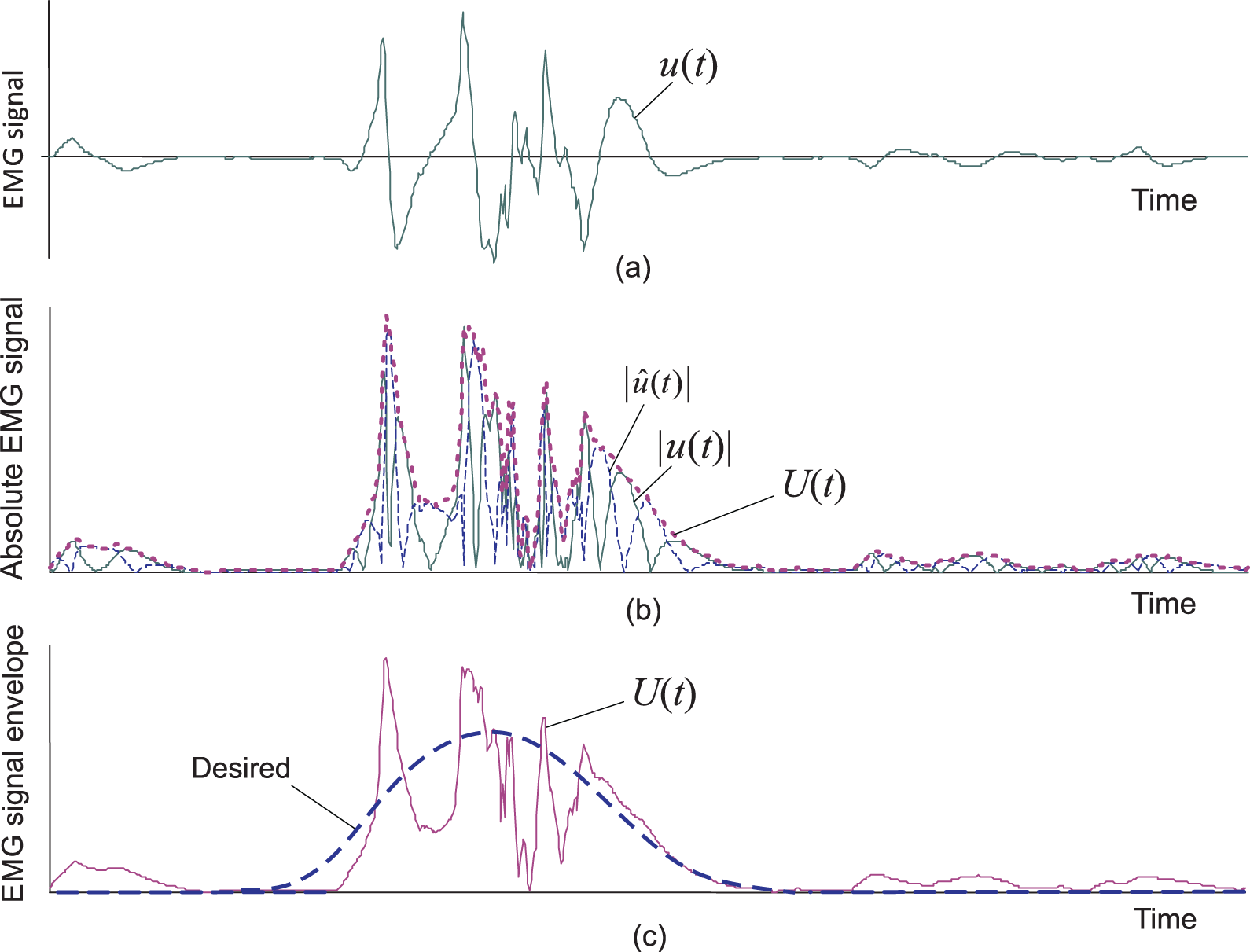
Figure 11.19 EMG signal: (a) measured EMG signal  composed by MUAPs, (b) Hilbert transform
  of
of  and envelope
  , and (c) extracted
  and desired EMG signal envelope.
A typical measured EMG signal ![]() , composed by low‐density MUAPs, is shown in Fig. 11.19a. An important function of the EMG signal is the envelope, which is used in robotic systems and prothesis control to achieve proper human‐robot interaction. The envelope
, composed by low‐density MUAPs, is shown in Fig. 11.19a. An important function of the EMG signal is the envelope, which is used in robotic systems and prothesis control to achieve proper human‐robot interaction. The envelope ![]() can be shaped by combining
can be shaped by combining ![]() with the Hilbert transform
with the Hilbert transform ![]() as shown in Fig. 11.19b. However, this may not always lead to a smooth shape due to multiple ripples. It should be noted that for the sake of stability of the proportional control of the artificial prothesis, it is desirable that the envelope has a Gaussian shape (Fig. 11.19c).
as shown in Fig. 11.19b. However, this may not always lead to a smooth shape due to multiple ripples. It should be noted that for the sake of stability of the proportional control of the artificial prothesis, it is desirable that the envelope has a Gaussian shape (Fig. 11.19c).
To keep the EMG envelope as close to Gaussian as possible, it was proposed in [120] to treat the ripples on the envelope (Fig. 11.19c) as CMN and use a general UFIR filter. Accordingly, the oversampled envelope ![]() was represented by the
was represented by the ![]() ‐state polynomial model [172] under the Gauss‐Markov CMN
‐state polynomial model [172] under the Gauss‐Markov CMN ![]() assumption as
assumption as
where ![]() is the
is the ![]() state vector and
state vector and ![]() is the scalar observation of
is the scalar observation of ![]() . For the polynomial approximation, entries of the system matrix
. For the polynomial approximation, entries of the system matrix ![]() are obtained using the Taylor series expansion as
are obtained using the Taylor series expansion as

and the number of states ![]() is chosen so that the best shaping is obtained.
is chosen so that the best shaping is obtained.
The observation ![]() of
of ![]() corresponds to the first state. Therefore, the observation matrix is assigned as
corresponds to the first state. Therefore, the observation matrix is assigned as ![]() . Matrix
. Matrix ![]() projects the
projects the ![]() noise
noise ![]() to
to ![]() . The scalar coloredness factor
. The scalar coloredness factor ![]() is determined during the testing phase to ensure the best shaping, and we notice that, by
is determined during the testing phase to ensure the best shaping, and we notice that, by ![]() , noise
, noise ![]() becomes white Gaussian. Noise
becomes white Gaussian. Noise ![]() is zero mean and white Gaussian,
is zero mean and white Gaussian, ![]() , with the variance
, with the variance ![]() .
.
Since the noise in ![]() is nonstandard, it is assumed that
is nonstandard, it is assumed that ![]() has zero mean with uncertain statistics and distribution. To run KF,
has zero mean with uncertain statistics and distribution. To run KF, ![]() is treated as zero mean and white Gaussian,
is treated as zero mean and white Gaussian, ![]() , with the covariance
, with the covariance ![]() , where
, where ![]() is the Kronecker symbol, and the property
is the Kronecker symbol, and the property ![]() for all
for all ![]() and
and ![]() . It is assumed that the estimate
. It is assumed that the estimate ![]() of
of ![]() under the ripples in
under the ripples in ![]() (Fig. 11.19c) will approach the Gaussian form if we assume that ripples are due to the CMN.
(Fig. 11.19c) will approach the Gaussian form if we assume that ripples are due to the CMN.
EMG Signals with Low‐Density MUAP
As an example, we consider an EMG signal composed of low‐density MUAPs that require the Hilbert transform to smooth the envelope [120]. The model in (11.47)–(11.49) is defined by two states, ![]() , and matrices
, and matrices
The EMG signal is taken from the “Elbowing” database [120], which contains samples collected from 11 subjects with knee abnormality previously diagnosed by a professional and 11 normal knees. Measurements are carried out using goniometry equipment MWX8 Datalog Biometrics with the sampling frequency ![]() , which corresponds to
, which corresponds to ![]() . Part of the database is shown in Fig. 11.20a. At the first step, the envelope is shaped using the Hilbert transform to represent “Data” as shown in Fig. 11.20b and Fig. 11.20c. Since information about noise is unavailable, the KF and UFIR filter are arbitrary tuned to produce consistent estimates with minimal variations regarding the desired smooth envelope and negligible time‐delays.
. Part of the database is shown in Fig. 11.20a. At the first step, the envelope is shaped using the Hilbert transform to represent “Data” as shown in Fig. 11.20b and Fig. 11.20c. Since information about noise is unavailable, the KF and UFIR filter are arbitrary tuned to produce consistent estimates with minimal variations regarding the desired smooth envelope and negligible time‐delays.
![Schematic illustration of EMG signal composed with low-density MUAP and envelope extracted using the Hilbert transform (Data) [120]: (a) EMG signal, (b) KF and UFIR filtering estimate, and (c) KF and UFIR filtering estimates modified for CMN.](https://imgdetail.ebookreading.net/2023/10/9781119863076/9781119863076__9781119863076__files__images__c11f020.png)
Figure 11.20 EMG signal composed with low‐density MUAP and envelope extracted using the Hilbert transform (Data) [120]: (a) EMG signal, (b) KF and UFIR filtering estimate, and (c) KF and UFIR filtering estimates modified for CMN.
The optimal horizon for a UFIR filter is measured as ![]() , which means a high oversampling rate. To tune KF, several similar datasets are analyzed, and it is concluded that the assumed noise has a standard deviation of about
, which means a high oversampling rate. To tune KF, several similar datasets are analyzed, and it is concluded that the assumed noise has a standard deviation of about ![]() . Since the average third state (acceleration) of the envelope is about
. Since the average third state (acceleration) of the envelope is about ![]() with a tolerance of about
with a tolerance of about ![]() or even more, the standard deviation of the process noise is set as
or even more, the standard deviation of the process noise is set as ![]() , which makes the KF estimate consistent with the UFIR estimate. With this filter setup, the extracted envelopes are sketched in Fig. 11.20b, and it turns out that even if the filters improve the envelope without significant time delays, there are still a lots of ripples, which require further smoothing.
, which makes the KF estimate consistent with the UFIR estimate. With this filter setup, the extracted envelopes are sketched in Fig. 11.20b, and it turns out that even if the filters improve the envelope without significant time delays, there are still a lots of ripples, which require further smoothing.
To get rid of the ripples in the envelope, it is next assumed that the measurement noise is colored and of Gauss‐Markov origin (11.49). Then the coloredness factor is set as ![]() to provide the best smoothing without significant time delay, the optimal horizon is measured as
to provide the best smoothing without significant time delay, the optimal horizon is measured as ![]() , and the GKF and UFIR filter modified for CMN are applied. What follows from the result shown in Fig. 11.20c is that the filters essentially suppress ripples and improve the envelope and that the latter finally better matches the desired Gaussian shape.
, and the GKF and UFIR filter modified for CMN are applied. What follows from the result shown in Fig. 11.20c is that the filters essentially suppress ripples and improve the envelope and that the latter finally better matches the desired Gaussian shape.
11.7 Summary
In this chapter, we looked at several practical uses of FIR state estimators, and one can deduce that the FIR approach can be extended to many other traditional and new challenging tasks. The aim was to demonstrate the difference between the FIR and IIR (KF) estimates obtained from real data. The following important points should be kept in mind.
Optimal estimators such as the OFIR filter and KF serve well when the model is process‐fit and the noise is Gaussian or near Gaussian. Otherwise, the UFIR state estimator may be more accurate. There are some boundary conditions that separate the scope of optimal and unbiased estimates in terms of accuracy and robustness. But this is a subtle matter that requires investigations in individual cases. Indeed, it is always possible to set some noise covariance, even heuristically and with no justification, to make the KF accurate, and there is always an optimal horizon ![]() that makes the UFIR estimate suboptimal. Therefore, the question arises, which is practically easier: to determine the noise covariances or
that makes the UFIR estimate suboptimal. Therefore, the question arises, which is practically easier: to determine the noise covariances or ![]() ? The answer depends on the specific problem, but it is obvious that it takes less efforts to determine the scalar
? The answer depends on the specific problem, but it is obvious that it takes less efforts to determine the scalar ![]() than the covariance matrix. Moreover, given the horizon length of
than the covariance matrix. Moreover, given the horizon length of ![]() , even not optimal, the UFIR state estimator becomes blind and therefore robust, which is highly required in many applications, especially industrial ones.
, even not optimal, the UFIR state estimator becomes blind and therefore robust, which is highly required in many applications, especially industrial ones.
We conclude this chapter by listing several modern and nontraditional signal processing problems that can be solved using FIR state estimation technologies, and note that this list can be greatly expanded.
11.8 Problems
- ML is pursued to estimate parameters such as mean and covariance of medical images for normality and abnormality employing a support vector machine. Since noise in images is non‐Gaussian, it seems that robust UFIR/median smoothing may be more efficient.
- In uncertain random environments, the FIR approach can help to solve the problem of estimating instantaneous speed and disturbance load torque in motors with higher robustness than standard KF‐based algorithms.
- To adapt the KF‐based state estimator to uncertain environments under disturbances, artificial neural networks (ANNs) are used in what is referred to as a neuro‐observer, which is an EKF‐based structure augmented by an ANN to capture the unmodeled dynamics. It looks like a robust UFIR‐based observer with adaptive horizon might be a more efficient solution.
- To estimate state‐of‐charge of lithium‐ion batteries, which is critical for electrical vehicles, adaptive
 filtering is used to eliminate bias errors. Instead, the
  FIR and especially UFIR filtering algorithms should be tested as more robust and stable.
 - To avoid the construction of new power plants, transmission lines, etc., the distributed generation (DG) approach has received a big attention. For optimal localization of several DGs under power losses, KF‐based algorithms are used. Since noise in a DG environment is typically non‐Gaussian, a robust UFIR state estimator may be the best choice.
- To estimate the size and location of a brain tumor, a massively parallel finite difference method based on the graphics processing unit is used together with a genetic algorithm to solve the inverse problem. To provide effective noise reduction on finite intervals, FIR state estimators can be built in to achieve greater accuracy.